

Abstract
Brain imaging genetics is an emergent research field where the association between genetic variations such as single nucleotide polymorphisms (SNPs) and neuroimaging quantitative traits (QTs) is evaluated. Sparse canonical correlation analysis (SCCA) is a bi-multivariate analysis method that has the potential to reveal complex multi-SNP-multi-QT associations. We present initial efforts on evaluating a few SCCA methods for brain imaging genetics. This includes a data synthesis method to create realistic imaging genetics data with known SNP-QT associations, application of three SCCA algorithms to the synthetic data, and comparative study of their performances. Our empirical results suggest, approximating covariance structure using an identity or diagonal matrix, an approach used in these SCCA algorithms, could limit the SCCA capability in identifying the underlying imaging genetics associations. An interesting future direction is to develop enhanced SCCA methods that effectively take into account the covariance structures in the imaging genetics data.
Index Terms: Sparse canonical correlation analysis, neuroimaging, genetics, data synthesis
1. INTRODUCTION
Recent advances in acquiring multi-modal brain imaging and genome-wide array data provide exciting new opportunities to study the influence of genetic variation on brain structure and function. Research in this emerging field, known as imaging genetics, aims to identify associations between genetic factors such as single nucleotide polymorphisms (SNPs) and quantitative traits (QTs) such as neuroimaging phenotypes. Typical imaging genetics methods include: (1) massive univariate analyses [1] to quickly discover single-SNP-single-QT associations, (2) regression analyses [2] to examine the joint effect of multiple SNPs on one or a few targeted QTs, and (3) bi-multivariate analyses [3, 4, 5] to examine complex associations between many SNPs and many QTs.
Sparse canonical correlation analysis (SCCA) [6] is a bi-multivariate analysis method that has been applied to both real [3] and simulated [4] imaging genetics data. Although SCCA produced promising results on relating hippocampal surface signals to candidate AlzGene SNPs [3], our recent SCCA analysis on relating brain-wide region of interest (ROI) measures (e.g., volume, thickness, gray matter density) to the AlzGene SNPs yielded unstable results. Following [4], which tested SCCA on simulated diffusion tensor imaging (DTI) and SNP data, here we propose a method to generate realistic SNP and brain ROI data with known underlying SNP-QT associations, test a few existing SCCA implementations on the data, compare their performance, and discuss future directions.
2. SPARSE CANONICAL CORRELATION ANALYSIS
We first describe the three SCCA algorithms evaluated in this work. Let n be the sample size, X (n × p matrix) be the genotype data containing p SNPs, and Y (n × q matrix) be the imaging data containing q QTs. CCA seeks linear combinations of variables in X and variables in Y, which are maximally correlated between Xwx and Ywy, that is:
| (1) |
where wx and wy are the canonical vector or weights.
Two major weaknesses of CCA are that it requires n to exceed p+q and that it produces nonsparse Aj and Bj which are difficult to interpret. To overcome these weaknesses, Witten et al. [6] proposed a penalized matrix decomposition (“PMD” in short) method by imposing L1 constraints onto wx and wy, which was ||wx|| ≤ c1 and ||wy|| ≤ c2. They assumed XTX = I and YTY = I, and implemented the PMD method by alternately performing the following two steps until convergence.
where P1 and P2 are the L1 penalty functions to yield wx and wy sparse. The first update takes the form , where S(x, Δ) = sgn(x)(|x| − Δ)+ is the soft thresholding operator and Δx ≥ 0 is chosen so that P1(wx) = c1. The second update takes a similar form by swapping x and y.
Parkhomenko et al. [7] developed a similar iterative algorithm as follows to implement SCCA.
| (2) |
where , and Σxy is the covariance matrix between X and Y. One major difference between this method and PMD is that a diagonal matrix instead of an identity matrix was used to approximate the covariance matrices Σxx and Σyy. For convenience, we call this algorithm as “DIAG” in short.
Parkhomenko et al. [7] further extended DIAG to adaptive SCCA (“ADAP” in short) by adopting the adaptive lasso method. Now the update rule becomes as follows:
| (3) |
where denotes the first singular vector obtained from a full singular value decomposition (SVD) of K. λwx and γ are sparseness parameters, which can be optimally tuned by nested cross validation. The update rule for is likewise.
3. SYNTHETIC DATA GENERATION MODEL
To evaluate the performances of the three SCCA methods, we implemented a method to create realistic imaging genetics data with known underlying correlation structures. The major steps were as follows. (1)We started with real imaging genetics data, i.e., a SNP set and an imaging QT set. (2) The SNP data set X was not altered and was directly used as our simulated genetics data. (3) We estimated the covariance structure of the QT data. (4) We synthesized a QT data set with the same covariance structure and call that background QT data Ybg. Since Ybg was randomly drawn from a Gaussian distribution with a specified covariance structure, it was reasonable to assume there was no relationship between X and Ybg (see Figure 4(a, c) for an example). (5) We used the method described below to introduce a correlation between multiple SNPs and multiple QTs. (6) We repeated Step 5 multiple times and incorporated these new correlations by altering the background QT data Ybg to yield our simulated imaging data Y.
Fig. 4.
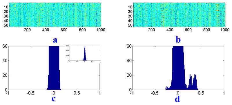
(a) Correlation matrix between SNP data X and QT background data Ybg. (b) Correlation matrix between SNP data X and simulated QT data Y after adding correlations. (c) Histogram of correlation coefficients between X and Ybg. (d) Histogram of correlation coefficients between X and Y.
Now we describe how to implement Step 5. Let XS be a subset of X and contains k SNPs of all the subjects. We can introduce a set of l correlated QTs YS using a method shown in Figure 1. In this synthetic correlation, l QTs are affected by k SNPs, and k ≪ p and l ≪ q. The error term can be used to adjust the strength of this k-SNP-l-QT correlation. In other words, the QT signal YS can be generated based on a subset of real SNP data XS as follows
Fig. 1.
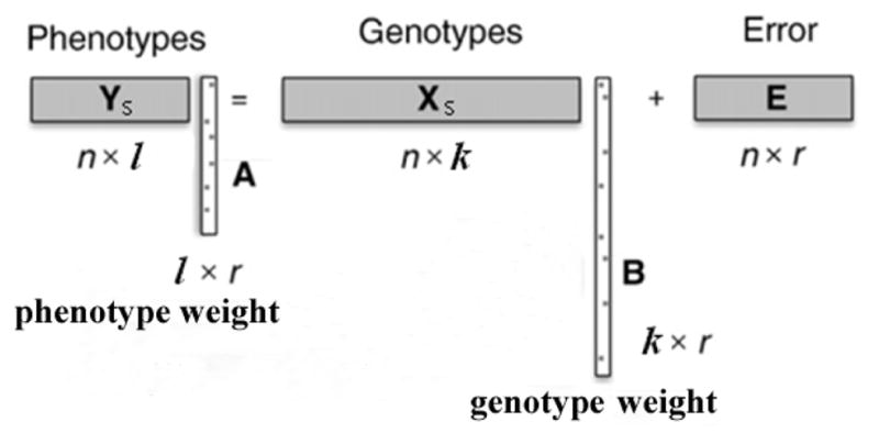
Synthetic correlation between k SNPs and l QTs.
| (4) |
where is the pseudo-inverse of AS and e is noise.
For each synthesized YSi, we can add αiYSi back to the corresponding columns in the background QT data Ybg to get the final simulated QT data Y. Parameter αi is specific to each synthesized correlation, and can be used to adjust the strengths between different synthetic correlations.
4. EXPERIMENTAL RESULTS
4.1. Real Data
The MRI and SNP data were downloaded from the Alzheimer’s Disease Neuroimaging Initiative (ADNI) database (www.adniinfo.org). One goal of ADNI has been to test whether serial MRI, PET, other biological markers, and clinical and neuropsychological assessment can be combined to measure the progression of mild cognitive impairment (MCI) and early AD. For up-to-date information, see www.adni-info.org.
Genotype data for the ADNI sample were collected using Illumina Human610-Quad Beadchip and underwent a standard quality control procedure. To accelerate the evaluation procedure, we focused on only the first 1000 (out of 9348) SNPs in chromosome 19, and 729 ADNI-1 non-Hispanic Caucasian participants were included in this study. To generate phenotype data, MRI scans at baseline for the ADNI-1 participants were pre-processed using FreeSurfer [1]. Bilateral means of 53 ROIs were calculated and used as original imaging QTs. The correlation structures and histograms of correlation coefficients of the real SNP and QT data are shown in Figure 2 and Figure 3(a, b).
Fig. 2.
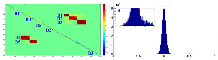
Shown in the left is the correlation matrix of the SNP data and two SNP sets selected for introducing SNP-QT correlations. One set contains three SNP blocks (shown as B1–B3), and the other contains two SNP blocks (shown as B4–B5); see also enlarged insets for correlations among these two sets of SNPs. Shown on the right is the histogram of correlation coefficients of the SNP data.
Fig. 3.
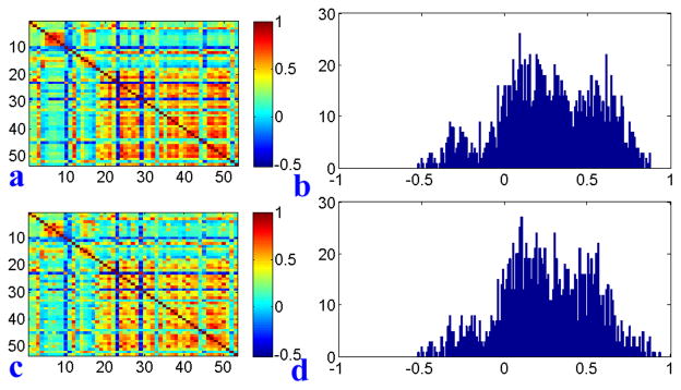
(a) Correlation matrix of real QT data. (b) Histogram of correlation coefficients of real QT data. (c) Correlation matrix of simulated QT data (SET1 with α=0.40). (d) Histogram of correlation coefficients of the simulated QT data.
4.2. Synthetic Data
To introduce synthetic correlations, we selected several SNP blocks from the genotype data, where a block indicated a set of highly correlated neighboring SNPs. Eq. 4 was used to generate the QT data. In our experiments, we created two different multi-SNP-multi-QT correlations. The first correlation was created between 12 SNP variables from three blocks ( and , see Figure 2 and Table 3) and 12 imaging variables from four blocks ( , containing 4, 4, 1 and 3 QTs respectively, see Table 3). The second correlation was created between 9 SNPs from two blocks ( and , see Figure 2 and Table 3) and 10 imaging variables from four blocks ( , containing 3, 3, 1 and 3 QTs respectively, see Table 3). Since Eq. 4 is under-determined, the QT blocks could be easily created so that QTs within each block have high correlation and QTs between blocks have low correlation.
Table 3.
Number of selected SNPs or QTs versus the total number of SNPs or QTs in the corresponding region. Note that the “All SNPs” or “All QTs” column contains the number of all selected SNPs or QTs, including both true positives and false positives. For SET3, there is only one set of results, and thus the two copies of “All SNPs” and “All QTs” columns are identical.
| SNP Data | QT Data | SNP Data | QT Data | ||||||||||||||||||||||||||||
|---|---|---|---|---|---|---|---|---|---|---|---|---|---|---|---|---|---|---|---|---|---|---|---|---|---|---|---|---|---|---|---|
|
| |||||||||||||||||||||||||||||||
| Region |
|
|
|
All SNPs |
|
|
|
|
All QTs |
|
|
All SNPs |
|
|
|
|
All QTs | ||||||||||||||
|
| |||||||||||||||||||||||||||||||
| Region size | 3 | 4 | 5 | 1000 | 4 | 4 | 1 | 3 | 53 | 5 | 4 | 1000 | 3 | 3 | 1 | 3 | 53 | ||||||||||||||
|
| |||||||||||||||||||||||||||||||
| SET1 Result | SET2 Result | ||||||||||||||||||||||||||||||
|
| |||||||||||||||||||||||||||||||
| PMA | α=0.8 | 3 | 4 | 5 | 44 | 3 | 4 | 1 | 3 | 25 | 5 | 4 | 36 | 3 | 2 | 1 | 2 | 18 | |||||||||||||
| DIAG | α=0.8 | 3 | 4 | 5 | 17 | 1 | 2 | 1 | 2 | 12 | 5 | 4 | 15 | 1 | 2 | 1 | 2 | 9 | |||||||||||||
| ADAP | α=0.8 | 3 | 4 | 5 | 17 | 1 | 1 | 1 | 2 | 10 | 5 | 4 | 13 | 1 | 2 | 1 | 1 | 8 | |||||||||||||
|
| |||||||||||||||||||||||||||||||
| PMA | α=0.4 | 3 | 3 | 4 | 54 | 3 | 3 | 1 | 2 | 36 | 4 | 4 | 42 | 2 | 2 | 1 | 2 | 25 | |||||||||||||
| DIAG | α=0.4 | 2 | 2 | 3 | 25 | 2 | 4 | 1 | 2 | 15 | 4 | 3 | 17 | 2 | 2 | 1 | 2 | 10 | |||||||||||||
| ADAP | α=0.4 | 2 | 2 | 2 | 20 | 3 | 2 | 1 | 2 | 11 | 3 | 3 | 14 | 2 | 2 | 1 | 1 | 9 | |||||||||||||
|
| |||||||||||||||||||||||||||||||
| SET3 Result | |||||||||||||||||||||||||||||||
|
| |||||||||||||||||||||||||||||||
| PMA | α1=0.8, α2=0.8 | 2 | 3 | 4 | 41 | 3 | 4 | 1 | 3 | 23 | 4 | 3 | 41 | 3 | 2 | 1 | 2 | 23 | |||||||||||||
| DIAG | α1=0.8, α2=0.8 | 3 | 4 | 4 | 21 | 2 | 3 | 1 | 2 | 18 | 4 | 4 | 21 | 2 | 2 | 1 | 2 | 18 | |||||||||||||
| ADAP | α1=0.8, α2=0.8 | 3 | 4 | 4 | 20 | 2 | 2 | 1 | 2 | 16 | 4 | 4 | 20 | 1 | 2 | 1 | 1 | 16 | |||||||||||||
|
| |||||||||||||||||||||||||||||||
| PMA | α1=0.4, α2=0.4 | 1 | 0 | 2 | 145 | 3 | 4 | 1 | 2 | 53 | 1 | 1 | 145 | 3 | 2 | 1 | 2 | 53 | |||||||||||||
| DIAG | α1=0.4, α2=0.4 | 0 | 1 | 0 | 32 | 3 | 3 | 1 | 2 | 21 | 1 | 1 | 32 | 2 | 2 | 1 | 2 | 21 | |||||||||||||
| ADAP | α1=0.4, α2=0.4 | 0 | 1 | 1 | 29 | 3 | 2 | 1 | 2 | 18 | 1 | 2 | 29 | 2 | 2 | 1 | 1 | 18 | |||||||||||||
We created three synthetic data sets: SET1 contained the first correlation only, SET2 contained the second correlation only, and SET3 contained both correlations. The correlation matrix and histogram of a SET1 type synthetic QT data set are shown in Figure 3(c, d), which are similar to those in the real QT data shown in Figure 3(a, b). Shown in Figure 4 are the pairwise SNP-QT correlations for simulated data before and after adding correlations.
4.3. SCCA Results
We applied three SCCA implementations (i.e., PMD, DIAG and ADAP) to three types of simulated imaging genetics data sets (i.e., SET1, SET2, and SET3). Based on the known underlying correlations, precision ( ) and recall ( ) were calculated to evaluate the method performances. Table 1 shows the results for SET1 and SET2, and Table 2 shows the results for SET3. DIAG and ADAP outperformed PMD on precision, while PMD performed better on recall. Between DIAG and ADAP, the ADAP performed slightly better for SET1 and SET2, and the results on SET3 were mixed. Table 3 shows the details on the number of selected SNPs in each block. While SNPs from some blocks could be all identified in some cases with a single strong correlation (e.g., SET1 or SET2 with α = 0.8), in cases with multiple or weak correlations (e.g., SET3 with α = 0.4) only very few SNPs could be identified from each block. QTs could not be all identified from each block in most cases. This indicates that the standard SCCA methods might not be sufficient to reveal imaging genetics associations while covariance structures within imaging or genetics (e.g., block diagonal in our data) are not adequately modeled. In addition, PMA produced many more false positives than DIAG and ADAP. In the extreme case (i.e., SET3 with α1 = 0.4 and α2 = 0.4), PMA returned all the QTs (53 out of 53) and many SNPs (145 out of 1000). But the false positives in DIAG and ADAP were relatively less. Note that DIAG and ADAP use diagonal matrix to approximate the covariance structure in the data, which contains more information than the identity matrix used in PMD. This further indicates that adequate modeling of covariance structure in the SCCA implementation is important.
Table 1.
Performance comparison: precision and recall values of testing PMD, DIAG and ADAP on SET1 and SET2.
| Precision | Recall | ||||||||
|---|---|---|---|---|---|---|---|---|---|
| α=0.4 | α=0.6 | α=0.8 | α=1.0 | α=0.4 | α=0.6 | α=0.8 | α=1.0 | ||
| SET1 | PMD | 0.211 | 0.286 | 0.333 | 0.458 | 0.792 | 0.833 | 0.875 | 0.917 |
| DIAG | 0.400 | 0.545 | 0.614 | 0.656 | 0.667 | 0.708 | 0.750 | 0.750 | |
| ADAP | 0.484 | 0.580 | 0.635 | 0.673 | 0.583 | 0.667 | 0.708 | 0.708 | |
| SET2 | PMD | 0.224 | 0.256 | 0.315 | 0.354 | 0.790 | 0.840 | 0.895 | 0.895 |
| DIAG | 0.519 | 0.566 | 0.625 | 0.682 | 0.632 | 0.737 | 0.790 | 0.790 | |
| ADAP | 0.522 | 0.603 | 0.667 | 0.701 | 0.632 | 0.684 | 0.737 | 0.737 | |
Table 2.
Performance comparison: precision and recall values of testing PMD, DIAG and ADAP on SET3
| Precision | Recall | ||||||
|---|---|---|---|---|---|---|---|
| α2=0.4 | α2=0.6 | α2=0.8 | α2=0.4 | α2=0.6 | α2=0.8 | ||
| PMD | α1=0.4 | 0.116 | 0.219 | 0.364 | 0.535 | 0.558 | 0.674 |
| PMD | α1=0.6 | 0.197 | 0.342 | 0.364 | 0.605 | 0.791 | 0.744 |
| PMD | α1=0.8 | 0.239 | 0.359 | 0.422 | 0.698 | 0.676 | 0.814 |
| DIAG | α1=0.4 | 0.358 | 0.421 | 0.556 | 0.442 | 0.535 | 0.628 |
| DIAG | α1=0.6 | 0.556 | 0.619 | 0.597 | 0.558 | 0.744 | 0.698 |
| DIAG | α1=0.8 | 0.597 | 0.615 | 0.674 | 0.651 | 0.721 | 0.767 |
| ADAP | α1=0.4 | 0.404 | 0.519 | 0.586 | 0.419 | 0.488 | 0.581 |
| ADAP | α1=0.6 | 0.542 | 0.624 | 0.634 | 0.512 | 0.698 | 0.674 |
| ADAP | α1=0.8 | 0.619 | 0.647 | 0.688 | 0.605 | 0.628 | 0.721 |
5. CONCLUSIONS
In this paper, initial efforts toward evaluating the sparse canonical correlation analysis (SCCA) methods in brain imaging genetics applications were presented. This included a data synthesis method to create a set of realistic imaging and genomic data with known underlying SNP-QT correlations, application of three SCCA algorithms to the synthetic data, and comparative study of their performances. These initial empirical results suggest that, although SCCA has the potential to reveal multi-SNP-multi-QT associations, its capability in effectively relating a set of correlated imaging measures to a set of correlated genomic measures is inadequate. One possible reason is that the existing implementations approximate the covariance matrices using either the identity matrix or diagonal matrices. One future topic is to evaluate additional SCCA implementations or develop new ones that take into account the covariance structures in the data (e.g., [4]). Once effective SCCA implementations are identified, another future topic is to apply those to real imaging genetics studies.
Acknowledgments
This research was supported by NIH R01 LM011360, U01 AG024904, RC2 AG036535, R01 AG19771, P30 AG10133, and NSF IIS-1117335 at IU, and by NIH R01 LM011360, R01 LM009012, and R01 LM010098 at Dartmouth.
References
- 1.Shen L, Kim S, et al. Whole genome association study of brain-wide imaging phenotypes for identifying quantitative trait loci in MCI and AD: A study of the ADNI cohort. Neuroimage. 2010;53(3):1051–63. doi: 10.1016/j.neuroimage.2010.01.042. [DOI] [PMC free article] [PubMed] [Google Scholar]
- 2.Hibar DP, Kohannim O, Stein JL, Chiang MC, Thompson PM. Multilocus genetic analysis of brain images. Front Genet. 2011;2:73. doi: 10.3389/fgene.2011.00073. [DOI] [PMC free article] [PubMed] [Google Scholar]
- 3.Wan J, Kim S, et al. Hippocampal surface mapping of genetic risk factors in AD via sparse learning models. MICCAI. 2011;14(Pt 2):376–83. doi: 10.1007/978-3-642-23629-7_46. [DOI] [PMC free article] [PubMed] [Google Scholar]
- 4.Chi EC, Allen GI, et al. Imaging genetics via sparse canonical correlation analysis. Biomedical Imaging (ISBI), 2013 IEEE 10th Int Sym on; 2013; pp. 740–743. [DOI] [PMC free article] [PubMed] [Google Scholar]
- 5.Le Floch E, et al. Significant correlation between a set of genetic polymorphisms and a functional brain network revealed by feature selection and sparse partial least squares. NeuroImage. 2012;63(1):11–24. doi: 10.1016/j.neuroimage.2012.06.061. [DOI] [PubMed] [Google Scholar]
- 6.Witten DM, Tibshirani R, Hastie T. A penalized matrix decomposition, with applications to sparse principal components and canonical correlation analysis. Biostatistics. 2009;10:515–533. doi: 10.1093/biostatistics/kxp008. [DOI] [PMC free article] [PubMed] [Google Scholar]
- 7.Parkhomenko E, Tritchler D, Beyene J. Sparse canonical correlation analysis with application to genomic data integration. Statistical Applications in Genetics and Molecular Biology. 2009;8:1–34. doi: 10.2202/1544-6115.1406. [DOI] [PubMed] [Google Scholar]