Abstract
Kinetic models are used extensively in science, engineering, and medicine. Mathematically, they are a set of coupled differential equations including a source function, otherwise known as an input function. We investigate whether parametric modeling of a noisy input function offers any benefit over the non-parametric input function in estimating kinetic parameters. Our analysis includes four formulations of Bayesian posteriors of model parameters where noise is taken into account in the likelihood functions. Posteriors are determined numerically with a Markov chain Monte Carlo simulation. We compare point estimates derived from the posteriors to a weighted non–linear least squares estimate. Results imply that parametric modeling of the input function does not improve the accuracy of model parameters, even with perfect knowledge of the functional form. Posteriors are validated using an unconventional utilization of the chi square test. We demonstrate that if the noise in the input function is not taken into account, the resulting posteriors are incorrect.
2 Introduction
Compartment models are widely used in science, engineering and medicine to mathematically model dynamical systems. They have been extensively used in molecular imaging with positron emission tomography (PET) and single photon emission computed tomography (SPECT) [15, 8] to estimate in vivo functional quantities such as blood flow [11], glucose metabolism for cancer imaging [2], Amyloid burden in the brain [10] to name a few. For more thorough review of molecular imaging please refer to [13, 6].
Dynamic PET studies involve imaging a radiotracer distribution over time. An imaging study begins when a radioactive tracer (radiotracer) is injected into a living subject. The radiotracer is then distributed in the tissues of the subject over time through the vascular system. Radiotracers are designed to interact with specific biological systems and processes in the subject. For instance, the radiotracer Flurpiridaz [5] is designed as a blood flow tracer for clinical cardiac imaging. Images reflecting the concentration of tracer are captured over sequential time frames. Each sequential image corresponds to the average concentration of the tracer during the time the image was acquired. These images provide information about radioactivity concentration as a function of time for every voxel in the image. Typically in cardiac perfusion imaging, a region of interest (ROI) which is a group of voxels corresponding to an imaged section of the myocardium is specified and time behavior of the average tracer concentrations in the ROI determined. This time behavior is usually referred to as a tissue time activity curve (TAC).
In compartmental models, compartments correspond to different physiological or biochemical states of the tracer. Rates that govern the transport of the tracer between compartments are referred to as kinetic parameters. Values of those parameters are indicative of the quantitative values that have direct correspondence to physical quantities such as blood flow, binding potential, or volume of distribution [6]. Estimated parameters describe the physiological system under study and may be used to determine whether the system is operating within specifications. For example, in diagnostic cardiac imaging using PET, the compartmental model [15] is used to estimate the blood flow (perfusion) in the myocardium. Values of tracer kinetic parameters are used as estimated and are strong predictors of clinical outcomes [11] and may guide physicians to choose optimal medical interventions.
In addition to the tissue TAC, an input function (concentration of the tracer in the blood plasma) is necessary to determine compartmental model parameters. Input functions for PET can be determined invasively by taking blood samples and measuring concentration of radioactive tracer. The clinical implementation of the blood sampling approach is not ideal due to complex logistics, increased cost and effort, increased risk, and inconvenience for the patient. The input function can also be acquired noninvasively from the image sequence by using a second ROI placed on a major artery or blood pool. For cardiac PET imaging this is straightforward as the left ventricle blood pool will always be in the field of view and placing the blood–pool ROI will be straightforward. In this work we use image–derived input functions.
Rate constants of the kinetic models are the parameters of interest and are typically estimated using a weighted non-linear least squares (WLS) approach in which the difference between the data and the model is minimized [12]. Both the tissue and input function TACs suffer from noise contamination which affect parameter estimates. Many currently used parameter estimation methods assume that the input function is noiseless [16, 12]. Others use an analytic model to fit to the input function TAC. The input function fit then serves as a “noiseless” input function. This input function fit is determined before the tissue data least squares fit is performed. The use of such a model of the input function is attractive because it imposes smoothness constraints on the input function, but the disadvantage is that the model may not represent the true input function in which case errors will be introduced and are difficult to track. To avoid this problem, non–parametric approaches that utilize the noisy input function [4] without assuming a model (functional form of the input function) can be used.
In this work we analyze four likelihoods which are used in the definition of the posteriors. A minimum–mean–square–error (MMSE) point estimate is used to determine bias, variance, and total error. We investigate the effect of the various models of the data (noise in the input function modeled/not modeled in the likelihood and the model of the input function used/not used) on the total error of one–compartment kinetic parameters. The result of the Bayesian methods are compared to standard non–linear optimization results and therefore a total of five estimation methods are studied. In addition to evaluation of point estimation using classical measures, we also evaluate validity of the resulting posteriors with a chi square distributed statistic for Bayesian methods. A Markov chain Monte Carlo (MCMC) simulation was used to numerically estimate posterior distributions.
The Bayesian methods are implemented based on four likelihood functions that are functions of 1) parameters of the input function and compartment models; 2) parameters of compartment model with estimated parameters for the input function; 3) parameters of compartment models with variance from the non–parametric input function factored into the covariance matrix of the residuals [4], and 4) parameters of compartment models with assumed noiseless non–parametric input function (noise in the input function is ignored).
3 Methods
3.1 Model
We use a general model of the data
| (1) |
where * denotes convolution, t is time, b(t) represents the TAC in some tissue ROI, a(t;ψ) is the input function which represents the concentration of the tracer in the arterial blood plasma. We assume for some of the methods used in this paper that a(t; ψ) can be represented by some analytic function parametrized by a vector of parameters ψ. h(t; θ) represents the impulse response function of the system model which depends on parameters θ.
Dynamic imaging with PET consists of acquiring a series of dynamic frames i with duration of τi. We assume the PET tomographic data is reconstructed and at least two regions of interest (tissue and blood) are placed on the reconstructed volumetric images. The average values of dynamic concentrations for each non-overlapping time frame in those ROIs are modeled by
| (2) |
| (3) |
where ti is the midpoint of the i-th time frame, A(ti) is the average concentration in the input function ROI for the i-th frame, and B(ti) is the average concentration for the tissue TAC. The actual PET measurements are denoted as α(ti) and β(ti) given as
| (4) |
| (5) |
where εA(i) and εB(i) are independent, normally distributed random variables such that εA(i) ~
 (0, σA(i)) and εB(i) ~
 (0, σB(i)). We assume that tissue and input noise are independent. This assumption is a limitation of the work presented in this paper, but it is not a limitation of the method in general. The correlation between different regions placed on the image (ROIs used to extract the tissue curves and input function) depends on many factors related to the reconstruction method [14].
The ROI noise variance is proportional to the imaged radioactivity concentration and inversely proportional to the frame time. Standard deviations are approximated [1] by
| (6) |
| (7) |
where CA and CB are constants that can be estimated from the data. The factor of 2ti/th is included to account for decay corrrection where th is the half life of the radiotracer. In practical applications A(ti) and B(ti) are unknown and therefore we approximate those in the calculation of the standard deviations by the sample values α(ti) and β(ti) [12].
3.2 Definition of Likelihoods
We analyze four approaches in defining the likelihood function. In all approaches, α(ti) and β(ti) are treated as independent random variables. Therefore we ignore the covariance between these terms however the inclusion of the covariance terms in the analysis is possible [4].
3.2.1 Likelihood with nuisance parameters: Method 1 (M1)
In approach one, the likelihood reflects the statistics of the tissue and input– function ROI measurements. Therefore we consider the probabilities of a joint distribution of α and β conditioned on the joint distribution of parameters θ and ψ. It follows that
| (8) |
where ρA = A − α and ρB = B − β are residuals of the model and measurements for input function and tissue, respectively. ϕα and ϕβ are covariance matrices of the input function and tissue measurements. The covariance matrices are diagonal with elements defined by Eqs. 6 and 7 implying that the noise in separate time frames is statistically independent which in practice holds very well [4]. In this formulation the θ are the parameters of interest and ψ constitute a set of parameters that are not of direct of interest and therefore are considered nuisance parameters.
3.2.2 Likelihood with estimated nuisance parameters: Method 2 (M2)
In the second approach the nuisance parameters are first estimated, ψ̂, and the likelihood is defined based on estimated values
| (9) |
where ψ̂ are estimated input function parameters. The weighted least squares algorithm [7] was used to obtain the estimate ψ̂.
3.2.3 Likelihood with estimated full covariance matrix: Method 3 (M3)
The third approach which takes into account noise in the input function is based on work of Huesman [4]. The most distinctive feature of this approach compared to the other two is that it does not use a parametrized input function. Instead the propagation of variance from the input function to residuals
 = Bα − β is modeled. Calligraphic font subscript
 is used to differentiate the residuals from the ones defined in the previous sections. In this approach the model of the TAC Bα is a function of the measurement α and therefore becomes a random variable. The covariance of this random variable can be calculated using some assumptions about the input function and can be added to covariance of β to provide the estimate of covariance of the residuals
 . We refer to the full covariance matrix which is a sum of the covariance of Bα and covariance of β as Σ. For more details about the derivation of this approach refer to the appendix [4]. The full covariance contains off–diagonal elements and it is a full rank, dense, positive definite, symmetric matrix. The full–covariance–matrix likelihood is formulated as
| (10) |
where Σ is the full covariance matrix.
3.2.4 Likelihood with estimated diagonal covariance matrix: Method 4 (M4)
In the fourth approach the noise in the input function is ignored and only the noise in the tissue TAC is taken into account when defining the likelihood. It follows that that likelihood is defined as
| (11) |
As in the likelihood with estimated full covariance described in Section 3.2.3, the non–parametric model of the input function is used.
3.3 Posteriors and Bayesian Point Estimators
Each of our four likelihood functions p1, p2, p3 and p4 is used with the same respective prior distributions assumed for θ and ψ to obtain the posteriors. In general, the priors represent beliefs about the values of parameters before the experiment. In this work we assumed that values of the parameters are a priori statistically independent and use non–informative priors by assigning equal beliefs that priors are true for parameters within an interval bounded by positive values. The prior is zero outside the interval. In clinical applications, expert opinion may be incorporated to shape priors. Additional studies are needed to determine the sensitivity to the prior.
Using priors defined above, likelihoods p1 through p4 described in the previous section, and Bayes theorem, closed forms of the posterior distributions through were obtained. We use the convention that the star–superscript indicates the posterior. The methods based on posteriors through will be referred to as M1 through M4, respectively.
For M1 through M4, we use a minimum mean square error (MMSE) point estimators. The MMSE point estimator is θ̂ = Ep*(θ) where Ep* denotes expectation over the posterior distributions.
3.4 Maximum Likelihood Method
As a reference we will compare the Bayesian methods to a standard optimization based estimator which is frequently used for estimation of kinetic parameters [15]. M5 is based on a weighted least squares fit of the model to the tissue TAC. In this method, the parametric input function is used and is determined from a WLS fit to the input function data[7]. The estimated input function is then used in the weighted least squares fit of the model to the data. Mathematically this estimator is defined as θ̂(β)WLS = maxθ p(β|θ)|ψ=ψ̂ where ψ̂ denotes a WLS estimate.
3.5 Numerical Methods for estimation of posteriors
We use a MCMC simulation to numerically estimate the posterior distribution. Starting values of the parameters θ0 and ψ0 for M1 and θ0 for M2 through M4 determined the initial Markov state. New values of parameters were generated from the prior distribution (selection step) and then the new state was accepted or rejected using acceptance probabilities derived form the likelihoods (acceptance step).
The selection step is performed by drawing a new value of parameter from a uniformly weighted interval [−d, d] centered about the current parameter value. If the new value fell outside the allowed interval by the prior specification it was reflected back into the interval.
For numerical stability and speed, acceptance of a new Markov state is based on the log–likelihoods of the new and old states. If a new state has a larger log–likelihood value, it is automatically accepted. If the new state has a lower log-likelihood, then the new state is accepted if the exponential of the ratio of new likelihood to old likelihood is larger than a randomly chosen number in the interval [0, 1]. Otherwise, it is not accepted. Effectively, a Metropolis–Hastings algorithm [9, 3] is implemented.
The value of parameters is logged for each step of the simulation. One and two dimensional histograms of parameter values are created from the logged data which after normalization represents marginalized posteriors of parameters. We found that the auto–correlation function of the data showed a correlation length of about 100, so our analysis included only every 100th data point in the chain.
A plot of the log–likelihood is used as a guide to determine when the Monte Carlo simulation has reached equilibrium. The iterations required to reach equilibrium, or the burn-in time, were not included in the analysis of posterior distributions.
3.6 Experiment
We test and compare the methods using a one–tissue compartment model including a blood fraction. The blood fraction takes into account the amount of tracer due to blood in the tissue ROI. We first generate the true noiseless input function based on the following model [4].
| (12) |
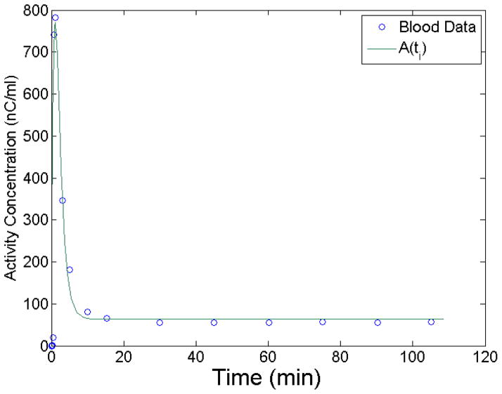
To determine realistic values of ψ̂ parameters that will be used in the simulation to generate the tissue curves, we integrate Eq. 12 over the τi to give A(ti). This simulates the noiseless input function. A(ti) was fit to experimental blood data using a weighted least squares algorithm. Figure 1 shows the least squares fit of A(ti) to sampled blood data.
Figure 1.
Input function model A(ti) least squares fit to blood data. The fit is used to determine A(ti), the noise-free input function.
Simulation of the measurement α was obtained by adding normally distributed noise with standard deviation σA. Estimated standard deviations of the input function used for calculation of likelihoods are where CA is a constant factor.
The simulated tissue curve, B(ti), was calculated using a one tissue compartment model including a blood fraction. The impulse response is given as
| (13) |
Simulation of the measurement β was obtained by adding normally distributed noise with standard deviation σB. For analysis, we use estimated standard deviations of the TAC calculated as where CB is a constant factor.
We analyze posteriors for two sets of constants (CA, CB) equal to (0.5, 1) and (2, 1) relating to low and high noise levels in the input function. For each set (CA, CB) 30 noise realizations of α and β were generated and analyzed. We made a trade–off between MCMC iterations and noise realizations, opting for more iterations in order to obtain a good approximations of the shapes of the posteriors. The code was written in MATLAB and was not optimized for speed. It took 8 hours to obtain a posterior for M3 which involves covariance matrix inversion in each Markov move.
We used 47 non–overlapping time frames with durations 16 × 15 seconds, 2 × 60 seconds, 10 × 120 seconds, and 23 × 300 seconds. The half life of F-18 was used, th = 109.8 minutes.
3.7 Figures of merit
3.7.1 Classical figures of merit
We use classical statistical measures of bias, standard deviation, and total error as figures of merit to asses the performance of point estimators. We define the bias vector for M1–M4 as where the sum is over N realizations of α and β, and θt are the true parameter values. θ̂ are the point estimates evaluated as the mean of the posterior for M1–M4, and the maximum likelihood for M5. We define the standard deviation of the estimator as where is the average value of the θ̂. We define total error as .
The error of the bias, Δb, is the standard error of the mean (SEM) of θ̂ distribution. We calculate the estimate of the SEM by bootstrapping with 1000 resamples from N = 30 values of θ̂. The SEM is the standard deviation of the bootstrap means. The error in s, Δs, is calculated from 1000 resamples of the standard deviation values. The error in
 is
where mathematic operations are defined pointwise.
3.7.2 Goodness–of–the–posterior figure of merit
In addition to a mean of the posterior, the methods presented in this work provide the approximation of the entire posterior distribution. In the Bayesian interpretation, the true value of parameters should be described by the posterior distribution. In order to test this hypothesis we use the χ2 test in an unconventional way.
The χ2 distribution with N degrees of freedom describes the distribution of the sum of squares of N variates drawn from the standard normal distribution. The χ2 test is used to determine the probability that a sample comes from the χ2 distribution. In our approach, we assume normality of the posteriors. The true value is then taken to be a sample from each of the N posterior distributions. This gives us N samples from a normal distribution from which we form N standardized normal samples. Our null hypothesis is that the sum of such samples is χ2 distributed.
Mathematically this can be summarized by defining a standardized random variable from the true parameter values θt, the point estimates θ̂, and the posterior standard deviations σ* as . The component-wise sum of Z, , is distributed as chi square with N = 30 degrees of freedom. We expect that the effect of including input function noise in the model should be large, which was confirmed with this test, and we were able to reject the null hypothesis using 30 samples.
4 Results and Discussion
4.1 Equilibrium
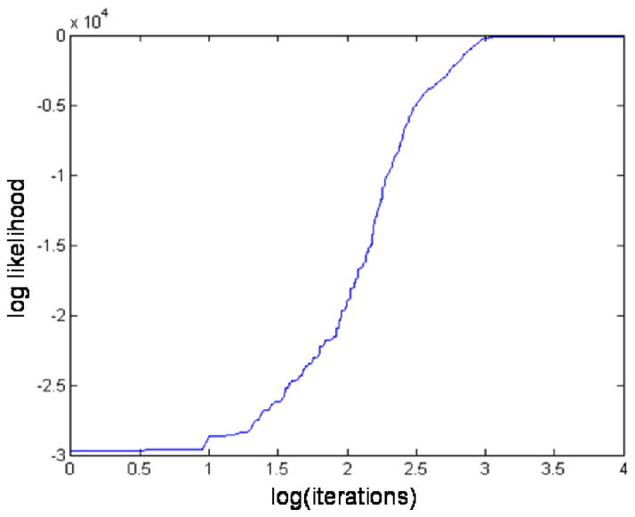
The Monte Carlo simulation reaches equilibrium evidenced by a leveling off of the log–likelihood. The approach to equilibrium is termed the burn–in period. Figure 2 shows a representative burn-in period for M1. After about 3,000 iterations, the log–likelihood levels off. For our analysis, we chose a burn–in period of 50,000 iterations after which we begin to record data. Note that based on Fig. 2 we chose an ample burn–in period as the log(50000) = 10.8.
Figure 2.
An example plot of the logarithm (log) of the likelihood showing the burn-in period. Values on the x-axis are the log of the simulation iteration. The likelihood levels off at about 3000 iterations. We use an ample burn–in period of 50000 iterations after which we start recording Markov Chain states.
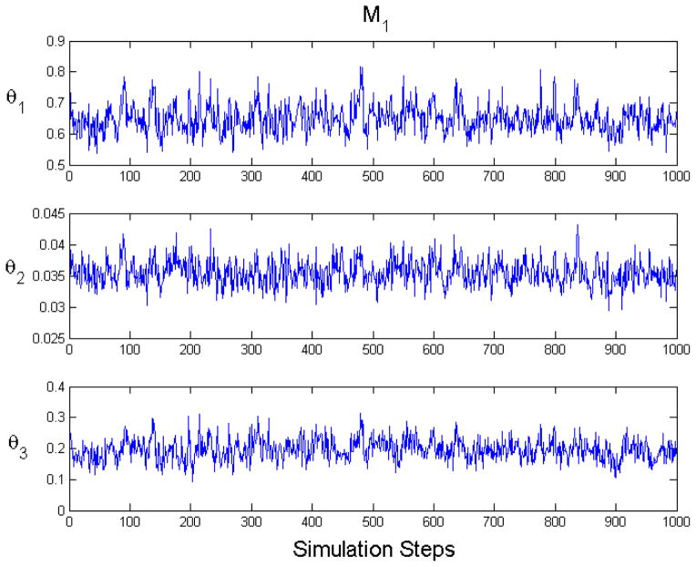
In Figure 3 we show an example of state mixing for M1. The plots account for burn in and auto–correlation.
Figure 3.
An example plot of equilibrium Markov chain Monte Carlo state mixing for M1 (CA = 2). These plots account for burnin and auto–correlation.
4.2 Evaluation of point estimates
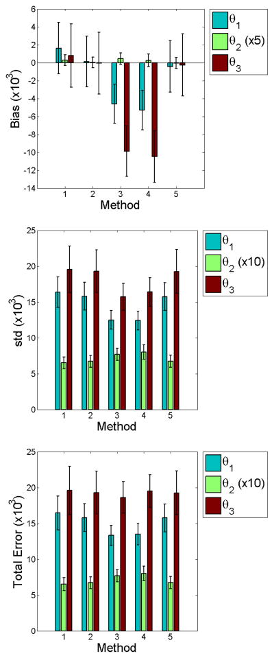
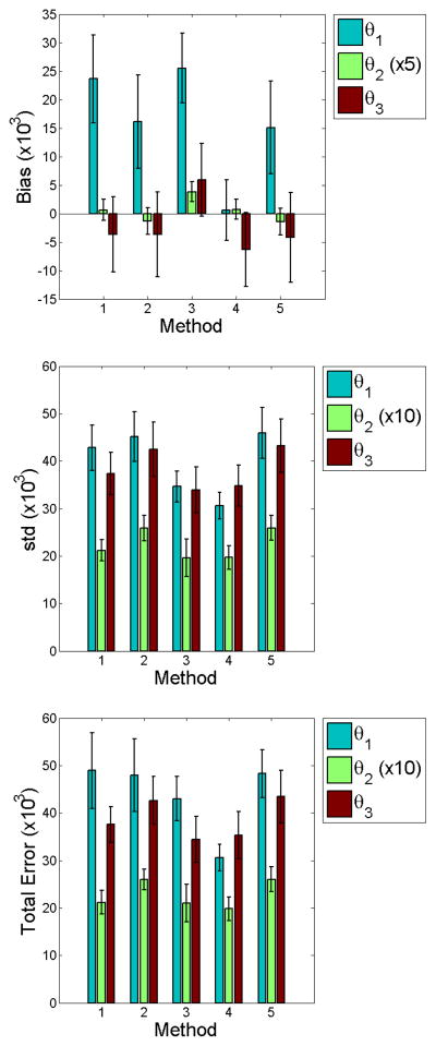
Figures 4 and 5 graphically show results of the computed statistics described in Section 3.7.1. We find no statistical significance of total error at low noise among the methods studied. We do note larger biases for M3 and M4. However, the smaller errors in both bias and standard deviation contribute to total errors of no significance. This implies that parametric modeling of the input function offers no clear benefit over non-parametric methods which do not model the input function. Comparison of M2 and M4 highlight this finding, since the only difference in the likelihood between these methods is whether the input function was or was not estimated. In the high noise case for M2 and M4, total errors for θ1 and θ2 imply that it may be more beneficial to use a non–parametric approach.
Figure 4.
Bar graphs of the point estimate statistics for low input function noise (CA = 0.5). We find no statistical difference in standard deviation and total error between methods. M3 and M4 show larger bias for θ2 and θ3. Smaller errors in both bias and standard deviation contribute to total errors of no significance.
Figure 5.
Bar graphs of the point estimate statistics for high input function noise (CA = 2). Comparison of total errors for M2 and M4 imply that it may be more beneficial to use a non–parametric approach.
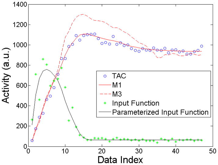
Figure 6 shows interesting M1 and M3 results for a single noise realization. Point estimates were used for the parametrized input function and data model, Eqs. 1 and 12. Clearly, M3 shows large deviations from the the TAC data. This deviation results from incorporation of the noisy input function data into the model as described in Sec. 3.2.3. Nonetheless, it is surprising that such a seemingly poor fit to the data is possible and contributes to produce no statistically significant differences in parameter estimates over the traditional methods when averaged over the noise ensembles.
Figure 6.
Plot of the TAC, M1, M3, input function, and parametrized input function for one noise realization (CA = 2). M3 shows significant departures from the data. These depeartures result from incorporation of the noisy input function inot the model.
4.3 Evaluation of posteriors
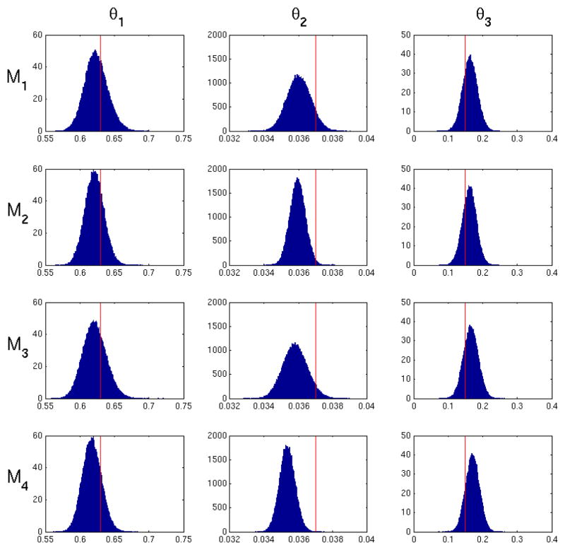
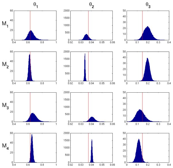
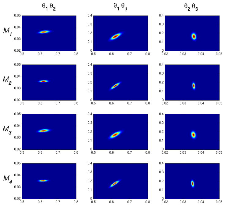
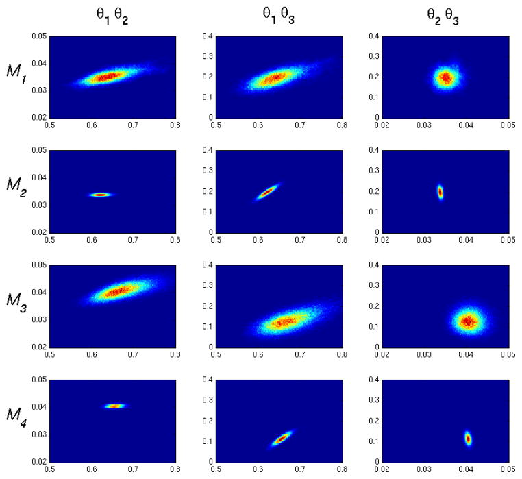
Figures 7 and 8 present examples of marginalized posterior probability densities of kinetic parameters for a low and high noise realization for M1–M4. The high noise histogram represents the same realization used in Figure 6. Table 1 shows the average posterior standard deviation for M1 through M4. All methods exhibit the expected increase in posterior variance from low noise to high noise. Within each noise level, M1 and M3 generally exhibit the largest posterior variance in values of all the methods. We expect to see a larger posterior standard deviation in M1 since uncertainty of the input function is taken into account in the likelihood in Eq. 8. In other words, Eq. 8 will give a range of values for a particular set of model parameters θ1 dependent on uncertainty in the input function. M3 has a posterior standard deviation similar to M1, since it depends on uncertainty in the input function which is incorporated into Σ. M2 generally has the smallest posterior variance, since fitting the input function underestimates the variance of Ψ̂ and therefore reduces total uncertainty. The resulting posterior is expected to be more precise, but does not represent the probability of the true value. Note that we used initial parameter values that matched the true ψ for fitting of the input function. Thus enabling the best possible outcome for input function estimation. In practice, the true form of the input function is unknown and true values of the input function parameters are unknown. Therefore in practical applications M1, M2 and M5 can only perform worse. M4 shows a posterior standard deviation very similar to M2, since uncertainty in the input function is not taken into account.
Figure 7.
Posterior probability density of the model parameters for M1–M4 for one low noise realization (CA = 0.5). The red line indicates the true parameter values. M1 and M3 exhibit the largest variance due to uncertainty in the input function. M2 has the smallest variance due to fitting the input function.
Figure 8.
Posterior probability density of the model parameters for M1–M4 for one high noise realization (CA = 2). The red line indicates the true parameter values. This is the same realization used for the data in Figure 6. M1 and M3 exhibit the largest variance due to uncertainty in the input function. M2 has the smallest variance due to fitting the input function.
Table 1.
Standard deviation of the posteriors for methods M1–M4. M1 and M3 exhibit the largest standard deviation due to uncertainty in the input function. M2 and M4 have the smallest standard deviation due to fitting the input function.
| Noise Level | θ1 (10−3) | θ2 (10−3) | θ3 (10−3) | |
|---|---|---|---|---|
|
| ||||
| 0.5 | M1 | 16.7 ± 0.2 | 0.709 ± 0.003 | 21.2 ± 0.1 |
|
|
||||
| M2 | 13.7 ± 0.2 | 0.464 ± 0.002 | 20.0 ± 0.1 | |
|
|
||||
| M3 | 16.4 ± 0.2 | 0.733 ± 0.003 | 21.2 ± 0.1 | |
|
|
||||
| M4 | 13.3 ± 0.1 | 0.463 ± 0.002 | 19.7 ± 0.1 | |
|
| ||||
| 2 | M1 | 41.3 ± 0.9 | 2.10 ± 0.03 | 31.7 ± 0.6 |
|
|
||||
| M2 | 14.3 ± 0.4 | 0.458 ± 0.006 | 20.1 ± 0.3 | |
|
|
||||
| M3 | 46.2 ± 1.1 | 2.23 ± 0.03 | 38.6 ± 0.7 | |
|
|
||||
| M4 | 13.9 ± 0.4 | 0.472 ± 0.006 | 20.0 ± 0.0 | |
Figures 9 and 10 show representative two dimensional density plots for low and high noise cases. We see correlations which qualitatively agree with the one compartment model impulse response given in Eq. 13. θ1 is positively correlated with θ2, since increasing the kinetics into the tissue compartment will generally require an increase of kinetics out of the compartment to match a decrease in tissue activity at longer times. θ1 is negatively correlated with θ3, as can be appreciated by observing that an increase in θ3 will make (1−θ3) smaller in the second term of Eq. 13 thus causing an increase of θ1 to compensate. Finally, θ2 is negatively correlated with θ3, since again a decrease in the (1 − θ3) will necessitate an increase in long time dynamics influenced by e−θ2t.
Figure 9.
Two dimensional posterior density plots for M1–M4, low noise (CA = 0.5). The figure column labels, θi θj, correspond to x and y axes in the plots column-wise. Correlations qualitatively agree with the impulse response in Eq. 13.
Figure 10.
Two dimensional posterior density plots for M1–M4, high noise (CA = 2). Correlations qualitatively agree with the impulse response in Eq. 13.
To analyze the posterior distributions we use the approach outlined in Section 3. Table 2 shows the χ2 values. In both low and high noise cases, χ2 for M2 and M4 show significant departures from a chi square distribution with 30 degrees of freedom at the 0.01 level of statistical significance. This implies that the posteriors for M2 and M4 do not represent the probabilities of true values. Our analysis reveals that M1 and M3 produce posteriors that pass the chi square test and therefore are likely to represent the true posterior distributions.
Table 2.
χ2 for methods M1–M4 from a one compartment model. The * indicates two-tailed statistical significance at the P = 0.01 level with 30 degrees of freedom. M1 and M3 show the hypothesis that the true values are “draws” from normal distributions with mean 0 and variance 1 cannot be rejected.
| Noise Level | θ1 | θ2 | θ3 | |
|---|---|---|---|---|
|
| ||||
| 0.5 | M1 | 0.9583 | 0.8057 | 0.8757 |
|
|
||||
| M2 | 1.330 | 1.993* | 0.9327 | |
|
|
||||
| M3 | 0.8547 | 1.068 | 1.021 | |
|
|
||||
| M4 | 1.389 | 3.061* | 1.278 | |
|
| ||||
| 2 | M1 | 1.147 | 1.037 | 1.572 |
|
|
||||
| M2 | 9.413* | 34.67* | 5.173* | |
|
|
||||
| M3 | 1.059 | 1.062 | 1.058 | |
|
|
||||
| M4 | 8.120* | 25.96* | 3.500* | |
5 Conclusion
We have analyzed point estimates of four formulations of the posterior, M1–M4, in a one compartment model and compared them to the commonly used non–linear weighted least squares estimation approach, M5. Two of the posteriors, M1 and M2, are dependent on a parametrized model of the input function while M3 and M4 are independent of an input function model. Our results indicate that parametric modeling of the input function provides no improvement in total error. In fact, our data show that for increased noise in the input function, modeling the input function may give less reliable results in terms of total error. This finding may have important practical implications, as it implies that modeling of the input function offers no significant benefits while at the same time reduces the robustness of the approach. Furthermore, input function models are vulnerable to misrepresentation of the functional form of the input function thereby impacting kinetic parameter estimation.
The analysis presented in this paper provides the estimates of posterior distributions. Aside from the point estimates derived from the posteriors these distributions can be used to estimate confidence sets or used in decision making with a loss function defined. However, we have shown that the noise in the input function has to be taken into account in order to obtain reasonable estimates of the posterior distribution. Methods M2 and M4 were shown to provide posteriors which are too narrow. This is the result of not incorporating noise in the input function in the likelihoods. Since M3 does not use a parametric input function and at the same time provides accurate posteriors, our findings suggest this method is a good candidate for Bayesian analysis of compartmental models in PET.
An important issue in Bayesian analysis is the selection of the prior. In this work we used a simple flat prior for simulation purposes. However in future work analyzing clinical data, we plan to use a more subjective approach by incorporating expert opinions and expectations of the values of kinetic parameters. We also plan to investigate prior sensitivity.
We performed an analysis of posteriors for M1–M4. Based on a chi square distributed statistic, we show that fitting the input function invalidates the resulting posterior.
Acknowledgments
This work was supported by NIH grants EB013180, HL106474, and EB016315.
7 Appendix
This appendix provides the basics of the derivation of the covariance matrix of residuals Σ used in the method M3. For more details on this method and details of the derivation refer to work of Huesman [4]. The main assumption is that the continuous input function a(t) can be approximated from the measurements α(ti) as follows
| (14) |
where Ii(t) is the indicator function equal to 1 when t is in time interval defined by the time frame i and 0 otherwise and T is the total number of time frames. The approximation above is equivalent to one used in [4] Eq. 16.
Using the above the the covariance of the residuals Σ can be calculated using
| (15) |
where H(θ) is a matrix of coefficients that depends on θ calculated using Eq. 14 and Eq. 1.
References
- 1.Chen Kewei, Huang Sung-Chen, Yu Dan-Chu. The effects of measurement errors in the plasma radioactivity curve on parameter estimation in positron emission tomography. Phys Med Biol. 1991;36:1183. doi: 10.1088/0031-9155/36/9/003. [DOI] [PubMed] [Google Scholar]
- 2.Gambhir SS. Molecular imaging of cancer with positron emission tomography. Nat Rev Cancer. 2002;2(9):683–93. doi: 10.1038/nrc882. [DOI] [PubMed] [Google Scholar]
- 3.Hastings WK. Monte carlo sampling methods using markov chains and their applications. Biometrika. 1970;57:97. [Google Scholar]
- 4.Huesman RH, Mazoyer BM. Kinetic data analysis with a noisy input function. Phys Med Biol. 1987;32:1569. doi: 10.1088/0031-9155/32/12/004. [DOI] [PubMed] [Google Scholar]
- 5.Huisman MC, Higuchi T, Reder S, Nekolla SG, Poethko T, Wester HJ. Initial characterization of an 18f-labeled myocardial perfusion tracer. J Nucl Med. 2008;49:630. doi: 10.2967/jnumed.107.044727. [DOI] [PubMed] [Google Scholar]
- 6.Innis RB, et al. Consensus nomenclature for in vivo imaging of reversibly binding radioligands. J Cereb Blood Flow Metab. 2007;27:1533–9. doi: 10.1038/sj.jcbfm.9600493. [DOI] [PubMed] [Google Scholar]
- 7.Dennis JE., Jr . Nonlinear Least Squares, State of the Art in Numerical Analysis. Academic Press; 1977. [Google Scholar]
- 8.Meyer Jeffrey H, Ichise Masanori, Yonekura Yoshiharu. An introduction to pet and spect neuroreceptor quantification models. J Nucl Med. 2001;42(2):755–763. [PubMed] [Google Scholar]
- 9.Metropolis N, Rosenbluth AW, Rosenbluth MN, Teller AH, Teller E. Equations of state calculations by fast computing machines. J Chem Phys. 1953;21:1087. [Google Scholar]
- 10.Mintun MA, Larossa GN, Sheline YI, Dence CS, Lee SY, Mach RH, Klunk WE, Mathis CA, DeKosky ST, Morris JC. [11c]pib in a nondemented population: potential antecedent marker of alzheimer disease. Neurology. 2006;67(3):446–52. doi: 10.1212/01.wnl.0000228230.26044.a4. [DOI] [PubMed] [Google Scholar]
- 11.Murthy VL, Naya M, Foster CR, Hainer J, Gaber M, Di Carli G, Blankstein R, Dorbala S, Sitek A, Pencina MJ, Di Carli MF. Improved cardiac risk assessment with noninvasive measures of coronary flow reserve. Circ. 2011;124:2215. doi: 10.1161/CIRCULATIONAHA.111.050427. [DOI] [PMC free article] [PubMed] [Google Scholar]
- 12.Muzic RF, Jr, Christian BT. Evaluation of objective functions for estimation of kinetic parameters. Med Phys. 2006;33(2):342–53. doi: 10.1118/1.2135907. [DOI] [PubMed] [Google Scholar]
- 13.Phelps Michael E. Molecular Imaging and Its Biological Applications. Springer; 2004. [Google Scholar]
- 14.Stute S, Carlier T, Cristina K, Noblet C, Martineau A, Hutton B, Barnden L, Buvat I. Monte carlo simulations of clinical pet and spect scans: impact of the input data on the simulated images. Phys Med Biol. 2011;56:6441–6457. doi: 10.1088/0031-9155/56/19/017. [DOI] [PubMed] [Google Scholar]
- 15.Watabe H, Ikoma Y, Kimura Y, Naganawa M, Shidahara M. Monte carlo sampling methods using markov chains and their applications. Ann Nuc Med. 2006;20:583. doi: 10.1007/BF02984655. [DOI] [PubMed] [Google Scholar]
- 16.Zhou Y, Aston JAD, Johansen AM. Bayesian model comparison for compartment models with applications in positron emission tomography. J App Stats. 2013;40:993. [Google Scholar]


