Differentially Private Synthesization of Multi-Dimensional Data using Copula Functions

Abstract

Differential privacy has recently emerged in private statistical data release as one of the strongest privacy guarantees. Most of the existing techniques that generate differentially private histograms or synthetic data only work well for single dimensional or low-dimensional histograms. They become problematic for high dimensional and large domain data due to increased perturbation error and computation complexity. In this paper, we propose DPCopula, a differentially private data synthesization technique using Copula functions for multi-dimensional data. The core of our method is to compute a differentially private copula function from which we can sample synthetic data. Copula functions are used to describe the dependence between multivariate random vectors and allow us to build the multivariate joint distribution using one-dimensional marginal distributions. We present two methods for estimating the parameters of the copula functions with differential privacy: maximum likelihood estimation and Kendall’s τ estimation. We present formal proofs for the privacy guarantee as well as the convergence property of our methods. Extensive experiments using both real datasets and synthetic datasets demonstrate that DPCopula generates highly accurate synthetic multi-dimensional data with significantly better utility than state-of-the-art techniques.

1. INTRODUCTION

Privacy preserving data analysis and publishing [14, 15, 3] has received considerable attention in recent years as a promising approach for sharing information while preserving data privacy. Differential privacy [14, 15, 22] has recently emerged as one of the strongest privacy guarantees for statistical data release. A statistical aggregation or computation is DP¹ if the outcome is formally indistinguishable when run with and without any particular record in the dataset. The level of indistinguishability is quantified by a privacy budget ε. A common mechanism to achieve Differential privacy is the Laplace mechanism [16] which injects calibrated noise to a statistical measure determined by the privacy budget ε, and the sensitivity of the statistical measure inuenced by the inclusion and exclusion of a record in the dataset. A lower privacy parameter requires larger noise to be added and provides a higher level of privacy.

Many mechanisms (e.g. [14, 18, 29]) have been proposed for achieving differential privacy for a single computation or a given analytical task and programming platforms have been implemented for supporting interactive differentially private queries or data analysis [28]. Due to the composibility of differential privacy [28], given an overall privacy budget constraint, it has to be allocated to subroutines in the computation or each query in a query sequence to ensure the overall privacy. After the budget is exhausted, the database can not be used for further queries or computations. This is especially challenging in the scenario where multiple users need to pose a large number of queries for exploratory analysis. Several works started addressing effective query answering in the interactive setting with differential privacy given a query workload or batch queries by considering the correlations between queries or query history [38, 8, 43, 23, 42].

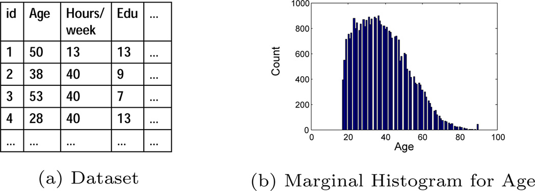
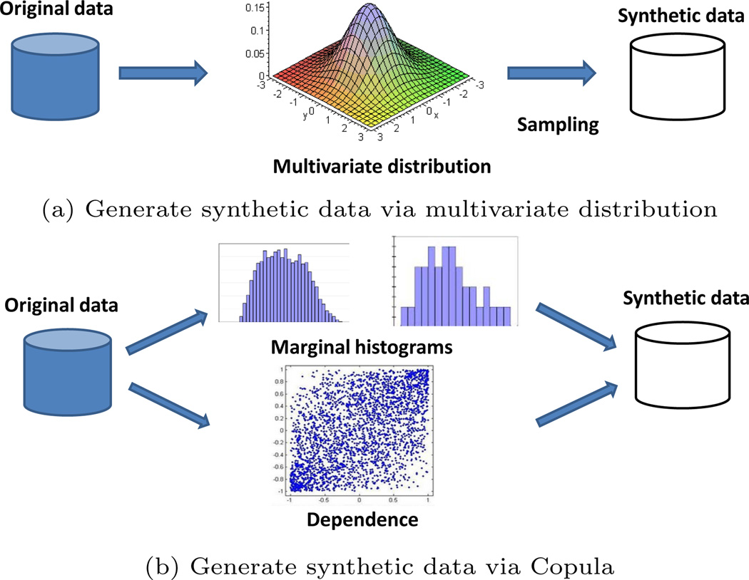
A growing number of works started addressing non-interactive data release with differential privacy (e.g. [5, 27, 39, 19, 12, 41, 9, 10]). Given an original dataset, the goal is to publish a DP statistical summary such as marginal or multi-dimensional histograms that can be used to answer predicate queries or to generate DP synthetic data that mimic the original data. For example, Figure 1 shows an example dataset and a one-dimensional marginal histogram for the attribute age. The main approaches of existing work can be illustrated by Figure 2(a) and classified into two categories: 1) parametric methods that fit the original data to a multivariate distribution and makes inferences about the parameters of the distribution (e.g. [27]). 2) non-parametric methods that learn empirical distributions from the data through histograms (e.g. [19, 41, 9, 10]). Most of these work well for single dimensional or low-order data, but become problematic for data with high dimensions and large attribute domains. This is due to the facts that:

1. The underlying distribution of the data may be unknown in many cases or different from the assumed distribution, especially for data with arbitrary margins and high dimensions, leading the synthetic data generated by the parametric methods not useful;

2. The high dimensions and large attribute domains result in a large number of histogram bins that may have skewed distributions or extremely low counts, leading to significant perturbation or estimation errors in the non-parametric histogram methods;

3. The large domain space ${\mathrm{\prod }}_{i=1}^m|A_i|$² (i.e. the number of histogram bins) incurs a high computation complexity both in time and space. For DP histogram methods that use the original histogram as inputs, it is infeasible to read all histogram bins into memory simultaneously due to memory constraints, and external algorithms need to be considered.

Figure 1.

Dataset vs. histogram illustration

Figure 2.

Synthetic data generation

Our contributions

In this paper, we present DPCopula, a novel differentially private data synthesization method for high dimensional and large domain data using copula functions. Copula functions are a family of distribution functions representing the dependence structure implicit in a multivariate random vector. Intuitively, any high-dimensional data can be modeled as two parts: 1) marginal distributions of each individual dimension, and 2) the dependence among the dimensions. Copula functions have been shown to be effective for modeling high-dimensional joint distributions based on continuous marginal distributions [31, 34, 4, 24]. They are particularly attractive due to several reasons. First, when we have more margins’ (Marginal distribution is shortened as margin in the paper) information than the joint distribution of all dimensions, they can be used to generate any joint distributions based on known margins and correlations among all dimensions. Second, they can be used to model non-parametric dependence for random variables. Further, we observe that existing DP histogram methods are efficient and effective for generating single dimensional marginal histograms, but not for high-dimensional data; and that the marginal distributions for discrete data in a large domain can be considered approximately continuous. Motivated by the above facts, the key idea of our proposed solution is to generate synthetic data from DP copula functions based on DP margins. We summarize our contributions below.

1. We propose a DPCopula framework to generate high dimensional and large domain DP synthetic data. It computes a DP copula function and samples synthetic data from the function that effectively captures the dependence implicit in the high-dimensional datasets. With the copula functions, we can separately consider the margins and the joint dependence structure of the original data instead of modeling the joint distribution of all dimensions as shown in Figure 2(b). The DPCopula framework allows direct sampling for the synthetic data from the margins and the copula function. Although existing histogram techniques can be used to generate DP synthetic data, post-processing is required to enforce non-negative histogram counts or consistencies between counts which results in either degraded accuracy or high computation complexity.

2. We present two methods, DPCopula-MLE (we shorten maximum likelihood estimation as MLE in the paper) and DPCopula-Kendall, for estimating parameters of the Gaussian copula function, a commonly used elliptical class of copula functions modeling the Gaussian dependence. We focus on semi-parametric Gaussian copula as most real-world high-dimensional data has been shown to follow the Gaussian dependence structure [31]. It can be used not only to model data with Gaussian joint distributions, but also data with arbitrary marginal distributions or joint distributions as long as they follow Gaussian dependence. DPCopula-MLE computes correlation among dimensions using DP MLE while DPCopula-Kendall computes DP correlation among dimensions using Kendall’s τ correlation which is a general nonlinear rank-based correlation.

3. We present formal analysis of differential privacy guarantees and computation complexity for the two DPCopula estimation methods. We also provide analysis of their convergence properties. Extensive experiments using both real datasets and synthetic datasets demonstrate that DPCopula generates highly accurate synthetic multi-dimensional data and significantly outperforms state-of-the-art techniques for range count queries.

2. RELATED WORK

Privacy-preserving synthetic data generation

The fundamental idea of data synthesization involves sampling data from a pre-trained statistical model, then release the sample data in place of the original data. Synthetic data can be used in preserving privacy and confidentiality of the original data. Numerous techniques have been pro-posed for generating privacy-preserving synthetic data (e.g. [21],[7]). But they do not provide formal privacy guarantees. Machanavajjhala et al. [27] presented a probabilistic DP Multinomial-Dirichlet (MD) synthesizer mechanism. They model the original map data using multinominal distribution with Dirichlet prior, and further enhance the utility via relaxing differential privacy and shrinking the domain space. Since the data is sparse, the noise added in the reduced domain still produce many outliers leading to limited utility of the synthetic data. Moreover, it guarantees probabilistic differential privacy instead of the strict differential privacy. Finally, the method is not applicable for data that does not follow multinomial distribution.

Differentially private histogram generation

Various approaches have been proposed recently for publishing differentially private histograms (e.g. [2, 40, 19, 41, 9, 10, 30, 1, 33]. Among them, the methods of [19] and [41] are designed for single dimensional histograms. The technique of [33] is proposed especially for two dimensional data. We discuss and compare the methods for multi-dimensional histograms below.

The method by Dwork et al. [13] publishes a DP histogram by adding independent Laplace random noise to the count of each histogram bin. While the method works well for low-dimensional data, it becomes problematic for high dimensional and large domain data. Barak et al. [2] uses Dwork’s method to obtain a DP frequency matix, then transforms it to the Fourier domain and adds Laplace noise in this domain. With the noisy Fourier coefficients, it employs linear programming to create a non-negative frequency matrix. But it [2] did not provide any empirical results. We do not include this method in our experimental comparison due to its high computational complexity. Xiao et al. [39] propose a Privelet method by applying a wavelet transform on the original histogram, then adding polylogarithmic noise to the transformed data. Cormode et al. [10] developed a series of filtering and sampling techniques to obtain a compact summary of DP histograms. The limitation is that if a large number of small-count non-zero entries exists in the histogram, it will give zero entries a higher probability to be in the final summary, leading to less accurate summary results. In addition, it needs carefully choosing appropriate values for several parameters including sample size and filter threshold. The paper did not provide a principled approach to determine them. Both the DPCube [40] and PSD [9] are based on KD-Tree partitioning. DPCube first uses Dwork’s method to generate a DP cell histogram and then applies partitioning on the noisy cell histogram to create the final DP histogram. PSD computes KD-tree partitioning using DP medians at each step. It has been shown in [9] that these two methods are comparable. However, for high-dimensional and large attribute domain data, either the level of partitioning will be high which results in high perturbation error or the distribution of each partition will be skewed which results in high estimation error. Acs et al. [1] study two sanitization algorithms for generating DP histograms. The EFPA technique improves the fourier perturbation scheme through tighter utility analysis while P-HP is based on a hierarchical partitioning algorithm. But there are limitations for high dimension data. When the number of bins in original histograms is extremely large, for EFPA, the parameter representing the histogram shape would be selected with high error; for P-HP, the accuracy of each partitioning step would have large perturbation error and the computation complexity would be proportional to the quadratic number of bins in the worst case.

The DiffGen method [30] releases differentially private generalized data especially for classification by adding uncertainty in the generalization procedure. Only predictor attributes are generalized for maximizing the class homogeneity homogeneity within each partition. For high-dimensional and large-domain data, the method has similar issues as the KD-partitioning methods. Because the method is designed for categorical attributes and for classification purposes, we will not include it in our experimental comparison.

Based on the discussion above, we will experimentally compare the proposed DPCopula method with the Privelet+ [39], Filter Priority (FP) method [10], PSD method [9], and P-HP method [1] as representatives of the general-purpose histogram methods.

Copula functions

The idea of copula was shown dating back to 1940’s, and the term copula was provided by the Sklar’s theorem [36] stating that copulas are functions connecting multivariate distributions to their one-dimension marginal distributions. An axiomatic definition of copulas can be found in Joe [20] and Nelsen [31]. Copula functions have been widely applied in statistics and finance in recent years (e.g. [34]).

3. PRELIMINARIES

Consider an original dataset D that contains a data vector (X₁, X₂, …, X_m) with m attributes. Our goal is to release differentially private synthetic data of D. For ease of reference, we summarize all frequently used notations in Table 1. Their definitions will be introduced as appropriate in the following (sub)sections.

Table 1.

Frequently used notations

Notation	Discription
D	original dataset
D̃	DP synthetic data
n	number of tuples in D
m	number of dimensions in D
(X1, …, Xm)	m-dimensional vector of D
H(x1, …, xm)	m-dimensional joint distribution
F̂j (xj)	empirical distribution of jth margin
F̃j (xj)	DP empirical distribution of jth margin
ρτ (Xj, Xk)	Kendall’s τ coefficient
ρ̂τ (Xj, Xk)	sample estimate of Kendall’s τ
ρ̃τ (Xj, Xk)	private estimate of Kendall’s τ
ρ(Xj, Xk)	the general correlation
ε1	privacy budget for margins
ε2	privacy budget for all correlations
Δ	sensitivity of Kendall’s τ
k	the ratio of ε1 and ε2
P̃	DP correlation matrix
(Ũ1, …, Ũm)	DP pseudo-copula data vector

3.1 Differential Privacy

Differential privacy has emerged as one of the strongest privacy definitions for statistical data release. It guarantees that if an adversary knows complete information of all the tuples in D except one, the output of a differentially private randomized algorithm should not give the adversary too much additional information about the remaining tuples. We say datasets D and D′ differing in only one tuple if we can obtain D′ by removing or adding only one tuple from D. A formal definition of Differential privacy is given as follows:

Definition 3.1 (ε-differential privacy [13]). Let 𝒜 be a randomized algorithm over two datasets D and D′ differing in only one tuple, and let 𝒪 be any arbitrary set of possible outputs of 𝒜 . Algorithm 𝒜 satisfies ε-differential privacy if and only if the following holds:

$$Pr[𝒜(D)\in 𝒪]\le e^{\epsilon }Pr[𝒜(D\prime )\in 𝒪]$$

Intuitively, differential privacy ensures that the released output distribution of 𝒜 remains nearly the same whether or not an individual tuple is in the dataset.

The most common mechanism to achieve differential privacy is the Laplace mechanism [13] that adds a small amount of independent noise to the output of a numeric function f to fulfill ε-differential privacy of releasing f, where the noise is drawn from Laplace distribution with a probability density function $Pr[\eta =x]=\frac{1}{2b}{e}^{-\frac{|x|}{b}}$. A Laplace noise has a variance 2b² with a magnitude of b. The magnitude b of the noise depends on the concept of sensitivity which is defined as follows.

Definition 3.2 (Sensitivity [13]). Let f denote a numeric function and the sensitivity of f is defined as the maximal L₁-norm distance between the outputs of f over the two datasets D and D′ which differs in only one tuple. Formally,

$${\mathrm{\Delta }}_f={\mathit{\text{max}}}_{D,D\prime }{\Vert f(D)-f(D\prime )\Vert }_1.$$

With the concept of sensitivity, the noise follows a zero-mean Laplace distribution with the magnitude $b=\frac{{\mathrm{\Delta }}_f}{\epsilon }$. To fulfill ε-differential privacy for a numeric function f over D, it is sufficient to publish f(D) + X, where X is drawn from $\mathit{\text{Lap}}(\frac{{\mathrm{\Delta }}_f}{\epsilon })$.

For a sequence of differentially private mechanisms, the composability [28] theorems guarantee the overall privacy.

Theorem 3.1 (Sequential Composition [28]). For a sequence of n mechanisms M₁, …, M_n and each M_i provides ε_i-differential privacy, the sequence of M_i provides $({\sum }_{i=1}^n{\epsilon }_i)$ -differential privacy.

Theorem 3.2 (Parallel Composition [28]). If D_i are disjoint subsets of the original database and M_i provides α-differential privacy for each D_i, then the sequence of M_i provides α -differential privacy.

3.2 The Copula function

Consider a random vector (X₁, …, X_m) with the continuous marginal cumulative distribution function (CDF) of each component being F_i(x) = P(X_i ≤ x), the random vector (U₁, …, U_m) = (F1(X1), …, F_m(X_m)) has uniform margins after applying the probability integral transform to each component. Then the copula function can be defined as follows:

Definition 3.3 (Copula and Sklar’s theorem [31]). The m-dimensional copula C : [0, 1]^m → [0, 1] of a random vector (X₁, …, X_m) is defined as the joint cumulative distribution function (CDF) of (U₁, …, U_m) on the unit cube [0, 1]^m with uniform margins:

$$C(u_1,\dots ,u_m)=P(U_1\le u_1,\dots ,U_m\le u_m)$$

where each U_i = F_i(X_i). Sklar’ theorem states that there exists an m-dimensional copula C on [0, 1]^m with F(x₁, …, x_m) = C(F₁(x₁), …, F_m(x_m)) for all x in ℝ̄^m. If F₁, …, F_m are all continuous, then C is unique. Conversely, if C is an m-dimensional copula and F₁, …, F_m are distribution functions, then $C(u_1,\dots ,u_m)=F(F_1^{-1}(u_1),\dots ,F_m^{-1}(u_m))$, where $F_i^{-1}$ is the inverse of marginal CDF F_i.

From definition 3.3, copula refers to co-behaviors of uniform random variables only; since any continuous distribution can be transformed to the uniform case via its CDF, this is the appeal of the copula functions: they describe the dependence without any concern of the marginal distributions. Here, dependence is a general term for any change in the distribution of one variable conditional on another while correlation is a specific measure of linear dependence [32] (e.g. Pearson correlation). Two distributions with the same correlations may have different dependencies. We use the rank correlation in our method and will discuss it later in this section. Although the data should be continuous to guarantee the continuity of margins, discrete data in a large domain can still be considered as approximately continuous as their cumulative density functions do not have jumps, which ensures the continuity of margins. We will discuss later how to handle small-domain attributes.

To study the accuracy of the copula-derived synthetic data, we introduce a convergence analysis on copulas, showing that the copula-derived synthetic data is arbitrarily close to the original data when the data cardinality is sufficiently large. Assume we have an original data D₀ with n records, {F₁₀, …, F_m0} being the original marginal distributions, C₀ be the original copula function (i.e. the original dependence), H₀ be the original joint distribution of the D₀. We also have t synthetic data D₁, …, D_t with {F_1t}, …, {F_mt} be a sequence of m one-dimensional marginal distributions and {C_t} be a sequence of copulas. Each {F_1i}, …, {F_mi} and C_i correspond to D_i, i ∈ {1, …, t} and are parameterized by the number of records of D_i. We have the following theorem:

Theorem 3.3 (Convergence of Copulas [25]). For every t in N⁺, a m-dimensional joint distribution function H_t is defined as H_t(x₁, …, x_m) := C_t(F_1t(x₁), …, F_mt(x_m)). Then the sequence {H_t} converges to H₀ in distribution, if and only if {F_1t}, …, {F_mt} converge to F₁₀, …, F_m0 respectively in distribution, and if the sequence of copulas {C_t} converges to C₀ pointwise in [0, 1]^m.

The Gaussian copula and Gaussian dependence

Although copula has several families, the elliptical class is the most commonly used, including Gaussian copula and t copula. In this paper, we focus on the semi-parametric Gaussian copula as it has better convergence properties for multi-dimensional data [26] and most real-world high-dimensional data follow the Gaussian dependence structure [31] that can be modeled by the Gaussian copula. We note that Gaussian copula is not to be confused with Gaussian distributions. The Gaussian copula can be used not only to model data with Gaussian joint distributions, but also data with arbitrary marginal distributions or joint distributions as long as they follow Gaussian dependence. For other types of data with special dependence structures, such as tail dependence, we can apply the t copula, the empirical copula and other copulas. Actually we can use many approaches to test the goodness-of-fit, such as Akaike’s Information Criterion (AIC) to identify the best copula. We leave designing DP t copula and other copulas and testing the goodness-of-fit for the best copula as our future work. Formally, we give the Gaussian copula and Gaussian dependence definitions as follows:

Definition 3.4 (The Gaussian Copula [6]). Deducing via Sklar’s theorem, a multivariate Gaussian density can be written as the product of two components: the Gaussian dependence and margins, denoted as

$${\mathrm{\Phi }}_{\mathit{P}}(\mathbf{x})=\underset{\mathit{\text{Gaussian dependence}}}{\underbrace{\frac{1}{|\mathit{P}{|}^{\frac{1}{2}}}\mathit{\text{exp}}\{-\frac{1}{2}{\varphi }^{-1}{(u)}^T({\mathbf{P}}^{-1}-\mathbf{I}){\varphi }^{-1}(u)\}}}\underset{\mathit{\text{Margins}}}{\underbrace{\prod _{i=1}^m\frac{\phi ({\varphi }^{-1}(u_i))}{{\sigma }_i}}}$$

where P is a correlation matrix³, I is the identity matrix, ϕ⁻¹ is the inverse CDF of a univariate standard Gaussian distribution, ϕ⁻¹ (u) = (ϕ⁻¹ (u₁), …, ϕ⁻¹ (u_m)), u_i = F_i(x_i), F_i(x_i) is Gaussian CDF with the standard deviation σ_i and φ is the standard Gaussian density, Φ_P denotes the multivariate Gaussian density. If we allow F_i(x_i) to be an arbitrary distribution function, we can obtain the density of Gaussian copula which is the Gaussian dependence part, denoted as $c_{\mathbf{P}}^{Ga}$, with the form

$$c_{\mathbf{P}}^{Ga}=|\mathbf{P}{|}^{-\frac{1}{2}}\mathit{\text{exp}}\{-\frac{1}{2}{\varphi }^{-1}{(u)}^T({\mathbf{P}}^{-1}-\mathbf{I}){\varphi }^{-1}(u)\}$$ (1)

From definition 3.4, the density function of Gaussian copula in equation (1) has no $1/\sqrt{{(2\pi )}^m}$ compared to that of Gaussian distribution because Gaussian copula allows arbitrary margins. The Gaussian copula does not necessarily have anything to do with Gaussian distributions that require all the margins to be Gaussian distributions. Rather, it represents the Gaussian dependence that arises from a random vector (U₁, …, U_m) with uniform margins. Each component of (U₁, …, U_m) may correspond to an arbitrary distribution F_i(X_i) before the probability integral transform is applied.

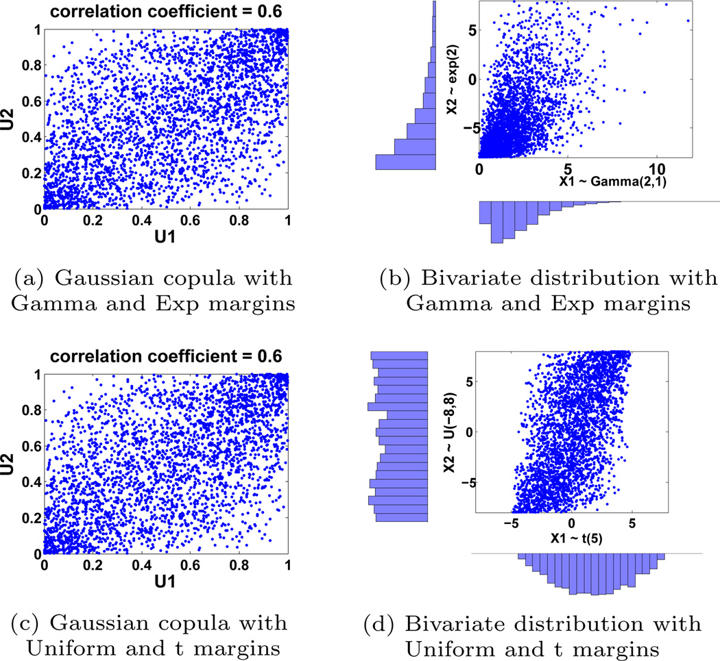
Figure 3 illustrates two bivariate Gaussian copula examples (i.e. two uniform random variables on [0, 1] with a Gaussian dependence structure) with the same correlation but different margins and the corresponding joint distribution. The same principle can be extended to more than two random variables. Figure 3(a) and (b) illustrates a scatter plot of a bivariate Gaussian copula with the exponential and gamma margins and a corresponding bivariate joint distribution with the attributes on the original domains. The scatter plots in Figure 3(c) and (d) is a bivariate Gaussian copula with uniform and t margins and its corresponding joint distribution. We can see that the joint distributions may be different due to different margins but the Gaussian copula scatter plots (i.e. Gaussian dependence) are the same with the same correlation. In other words, the dependence of data can be modeled independently from the margins. While real-world high dimensional data may have different marginal or joint distributions, most data follow the Gaussian dependence which can be modeled by Gaussian copula with different correlations.

Figure 3.

Gaussian copula vs. multivariate distribution

Estimation of the Gaussian copula

Since there are unknown parameters which are margins and P in the copula function, they can be estimated based on input data. The steps of estimation are as follows. First, the data is transformed to pseudo-copula data on [0, 1]^m by the non-parametric estimation method to estimate the marginal CDF. Assume X_j = (X_1,,j, …, X_n,j)^T is the jth data vector of (X₁, …, X_m), the empirical marginal CDF F_j on the jth dimension can be estimated by

$${\mathrm{F̂}}_j=\frac{1}{n+1}\sum _{i=1}^n{1}_{\{X_{i,j}\ge x\}}$$ (2)

where F̂_j is the empirical distribution function of X_j. Here n+1 is used for division to keep F̂_j lower than 1. Then, we can generate the jth-dimension pseudo-copula data by

$${\mathbf{Û}}_j={({\mathrm{F̂}}_j(X_{1,j}),\dots ,{\mathrm{F̂}}_j(X_{n,j}))}^T$$ (3)

Once we get the pseudo-copula data, there are two methods to estimate the correlation matrix P. The first method is directly using maximum likelihood estimation with the pseudo-copula data as input [6], named asMLE in our paper. However, maximizing the log likelihood function is specially difficult in multi-dimensions. For this reason, estimation based on dependence measure is of practical interest.

The second method is to estimate the correlation matrix P based on Kendall’s τ correlation coefficients between dimensions. From the original data vectors, we can estimate ρ_τ (X_j, X_k) by calculating the standard sample Kendall’s τ coefficient ρ̂_τ (X_j ;X_k) (see Section 3.2.3). Due to [6], the estimator of the general correlation coefficient, ρ(X_j, X_k), is given by

$$\rho ({\mathbf{X}}_j,{\mathbf{X}}_k)=\mathit{\text{sin}}(\frac{\pi }{2}{\mathrm{\rho ̂}}_{\tau }({\mathbf{X}}_j,{\mathbf{X}}_k))$$ (4)

In order to estimate the entire correlation matrix P, we need to obtain all pairwise estimates in an empirical Kendall’ τ matrix ${\mathbf{R}}_{\tau }(R_{jk}^{\tau }={\mathrm{\rho ̂}}_{\tau }({\mathbf{X}}_j,{\mathbf{X}}_k))$, then build the estimator $\mathbf{P̂}=\mathit{\text{sin}}(\frac{\pi }{2}{R}^{\tau })$ with all diagonal entries being 1.

Kendall’s τ rank correlation

Kendall’s τ rank correlation is a well-accepted rank correlation measure of concordance for bivariate random vectors. The definition of Kendall’s τ is given as follows:

Definition 3.5 (Kendall’s τ rank correlation [11]). The population version of Kendall's τ rank correlation has the form:

$${\rho }_{\tau }({\mathit{X}}_j,{\mathit{X}}_k)=E(\mathit{\text{sign}}(x_{i_1,j}-x_{i_2,j})(x_{i_1,k}-x_{i_2,k}))$$

where (x_i1,j, x_i1,k) and (x_i2,j, x_i2,k) are two different independent pairs with the same distribution. In practice, we can estimate ρ_τ (X_j, X_k) using ρ̂_τ (X_j, X_k) with the form ${\left(\begin{array}{c}\hfill n\hfill \\ \hfill 2\hfill \end{array}\right)}^{-1}{\sum }_{1\le i_1<i_2\le n}\mathit{\text{sign}}(x_{i_1,j},x_{i_2,j})(x_{i_1,k},x_{i_2,k})$ We shorten Kendall’s τ rank correlation as Kendall’s τ. We choose to use Kendall’s τ instead of other correlation metrics such as Pearson or Spearman because it can better describe more general correlations while Pearson can only describe the linear correlation and has better statistical properties than Spearman.

4. DPCOPULA

Under differential privacy, we propose two DPCopula algorithms for estimating Gaussian copula functions based on multi-dimensional data, namely DPCopula using MLE (DPCopula-MLE) and DPCopula using Kendall’s τ (DPCopula-Kendall). The general idea is to estimate marginal distributions and the gaussian copula function based on the original multivariate data, then sample synthetic data from this joint distribution while preserving ε-differential privacy. In this section, we first present the methods of DPCopula-MLE and DPCopula-Kendall with privacy proofs and complexity analysis, then analyze their convergence properties. Finally, we present a DPCopula hybrid method to handle small-domain attributes.

4.1 DPCopula-MLE

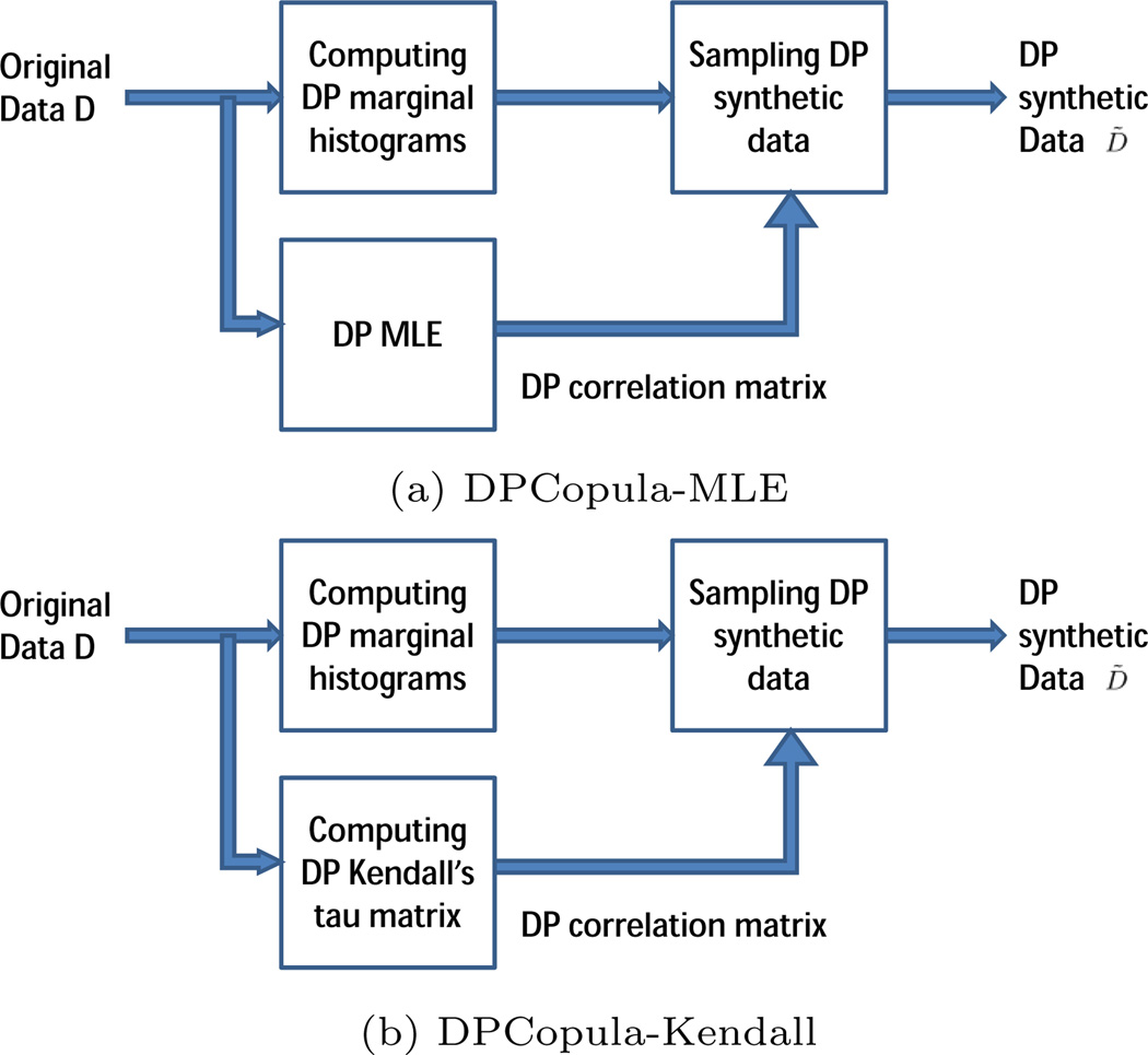
One basic method of DPCopula is to first compute DP marginal histograms, then estimate DP correlation matrix using the DP MLE method proposed by Dwork [17], then sample DP synthetic data. We illustrate this algorithm schematically in Figure 4(a). Algorithm 1 presents the steps of DPCopula-MLE. We present the details of each step below.

Figure 4.

DPCopula Overview

Computing DP marginal histograms

As a first step, we compute DP marginal histograms for each attribute. There are several state-of-the-art techniques for obtaining one-dimensional DP histograms effectively and efficiently, such as PSD, Privelet [39], NoiseFirst and StructureFirst [41], EFPA [1]. Here we use EFPA to generate DP marginal histograms which is superior to other methods. We note that an important feature of DPCopula is that it can take advantage of any existing methods to compute DP marginal histograms for each dimension, which can be then used to obtain DP empirical marginal distributions.

Algorithm 1.

DPCopula-MLE algorithm

Input: Original data vector D = (X1, …, Xm), and privacy budget ε.

Output: Differentially private synthetic data D̃ Create a differentially private marginal histogram with privacy budget $\frac{{\epsilon }_1}{m}$ for each dimension Xj, j = 1, …, m, in the original data vector to obtain DP empirical marginal distribution (Ũ1, …, Ũm) by equation (2); Use DP MLE to estimate the DP correlation matrix P̃ with privacy budget $\frac{{\epsilon }_2}{\left(\begin{array}{c}\hfill m\hfill \\ \hfill 2\hfill \end{array}\right)}$ for each correlation coefficient and ε2 = ε − ε1; Sample DP synthetic dataset D̃ by algorithm 3.

DP MLE

In step 2, we fit a Gaussian copula to the pseudo copula data generated from original data using equation 2 and 3, then use the DP MLE method to compute DP correlation matrix P̃. Our DP MLE method uses the similar idea with [17]. Algorithm 2 presents the general idea of DP MLE. It first divides the D horizontally into l disjoint partitions of $\frac{n}{l}$ records each, computes the MLE coefficient estimator on each partition, and then releases the average of these estimates plus some small additive noise. Here the sensitivity of each coefficient is $\frac{2}{l}$, for the diameter of each coefficient is 2. The value of l should be larger than $\left(\begin{array}{c}\hfill m\hfill \\ \hfill 2\hfill \end{array}\right)/0.025{\epsilon }_2$ which requires a large data cardinality for high dimensions. Algorithm 2 guarantees ε₂ differential privacy due to theorem 3.2 because each partition that is disjoint with each other preserves ε₂ differential privacy.

Algorithm 2.

DP MLE

Input: Original data vector D = (X1, …, Xm), privacy budget ε2, and k ∈ N+.

Output: Differentially private correlation matrix estimator P̃ Divide D horizontally into l disjoint partitions D1, …, Dl with each partition having $b=\frac{n}{l}$ tuples; For each partition Dt, t ∈ 1, …, l: $${\mathbf{P̃}}^t=\underset{P_{ij}\in \mathrm{\Theta }}{\text{arg max}}\sum _{r=(i-1)b+1}^{rb}\mathit{\text{log}}{\mathrm{C}}_{\mathbf{P}}^{Ga}(x_1^r,\dots ,x_m^r)$$ where ${\mathrm{C}}_{\mathbf{P}}^{Ga}$ represents the density of Gaussian copula. For each Pij ∈ [−1, 1], i, j ∈ 1, …, m Compute the average value through ${\mathrm{P̄}}_{ij}=\frac{1}{l}{\sum }_l^{t=1}{P}_{ij}^t$, Then inject Laplace noise to P̄ij and obtain DP P̃ij as $${\mathrm{P̃}}_{ij}={\mathrm{P̄}}_{ij}+\mathit{\text{Lap}}[\frac{\left(\begin{array}{c}\hfill m\hfill \\ \hfill 2\hfill \end{array}\right)\mathrm{\Lambda }}{l{\epsilon }_2}]$$ where Λ is the diameter of each correlation coefficient space Θ with a value of 2; Collect all P̃ij to constitute the DP correlation matrix estimator P̃

Sampling DP synthetic data

In step 3, we build a joint distribution based on definition 3.4 using the DP marginal histograms from step 1, and DP correlation matrix estimator P̃ from step 2, then sample data points from the joint distribution. The procedure of sampling DP synthetic data is given in Algorithm 3.

Privacy Properties

We present the following theorem showing the privacy property of the DPCopula-MLE algorithm.

Algorithm 3.

Sampling DP synthetic data

Input: DP marginal histograms and DP correlation matrix P̃

Output: DP synthetic data D̂ Generate DP pseudo-copula synthetic data (T̃1, …, T̃m): Generate a multivariate random number vector (X̃1, …, X̃m) in an arbitrary domain following the gaussian joint distribution Φ(0, P̃), where P̃ is returned by step 2 of Algorithm 1; Transform (X̃1, …, X̃m) to (T̃1, …, T̃m) ∈ [0, 1]n × m, where T̃j = ϕ(X̃j),j = 1, …, m and ϕ(X̃j) is the standard gaussian distribution; Compute DP synthetic data D̃ as follows: $$\mathrm{D̃}=({\mathrm{F̃}}_1^{-1}({\mathbf{T̃}}_1),\dots ,{\mathrm{F̃}}_m^{-1}({\mathbf{T̃}}_m))$$ where ${\mathrm{F̃}}_j^{-1}$ is the inverse of DP empirical marginal distribution function generated from the jth DP marginal histogram, and in the domain of the original dataset.

Theorem 4.1. Algorithm 1 guarantees ε - differential privacy.

Proof. Step 1 guarantees ε₁ differential privacy due to theorem 3.1. Step 2 guarantees ε₂ differential privacy due to [17]. Algorithm 1 guarantees ε₁ + ε₂ = ε differential privacy due to theorem 3.1.

Computation complexity

For the space complexity, the DPCopula-MLE algorithm takes O(mn) (i.e. the size of the original dataset), where m is the number of dimensions, n is the number of records in the original dataset. For the time complexity, computing all DP marginal histograms take $O({\sum }_{i=1}^m(A_i\mathit{\text{log}}{A}_i+n))=O(mA\mathit{\text{log}}A+mn)$ due to [1], where A = max{A₁, …, A_m}. DP MLE takes $O(l\times \frac{m^2{n}^2}{l^2})=O(\frac{m^2{n}^2}{l})$. DPCopula-MLE takes O(mAlogA + m²n²/l).

4.2 DPCopula-Kendall

In this section, we first present the key steps of DPCopula-Kendall and then provide formal proof for the privacy guarantee. Figure 4(b) illustrates the process of DPCopula-Kendall. Algorithm 4 presents the detailed steps of DPCopula-Kendall. From the key steps of algorithm 4, we can see that the differential privacy guarantee relies on step 1 and step 2, which share the privacy budget. As step 1 and step 3 of algorithm 4 are the same with algorithm 1, we only present the details of step 2 below.

Algorithm 4.

DPCopula-Kendall’s τ algorithm

Input: Original data vector (X1, …, Xm) containing m attributes, privacy budget ε

Output: Differentially private synthetic data D̃ Compute a differentially private marginal histogram with the privacy budget $\frac{{\epsilon }_1}{m}$ for each Xi in D ; Compute the DP correlation matrix P̃ using algorithm 5 with privacy budget $\frac{{\epsilon }_2}{\left(\begin{array}{c}\hfill m\hfill \\ \hfill 2\hfill \end{array}\right)}$ for each correlation coefficient, and ε2 = ε − ε1; Sample DP synthetic data D̃ by algorithm 3.

Computing differentially private correlation matrix

The differentially private estimator P̃ of the general correlation matrix is estimated by calculating noisy pairwise Kendall’ τ correlation coefficients matrix. From the original data vector (X₁, …, X_m), we can compute a noisy Kendall’s τ coefficient of any arbitrary two attributes X_j and X_k by the standard sample Kendall’s τ coefficient ρ̃_τ (X_j, X_k) using Laplace mechanism that guarantees ε₂-differential privacy. We then construct a noisy Kendall’ τ matrix ρ̃_τ with each element defined by ${\mathrm{\rho ̃}}_{jk}^{\tau }={\mathrm{\rho ̃}}_{\tau }({\mathbf{X}}_j,{\mathbf{X}}_k)$. Finally, we construct the noisy correlation matrix estimator as $\mathbf{P̃}=\mathit{\text{sin}}(\frac{\pi }{2}{\mathrm{\rho ̃}}_{\tau })$ with all diagonal entries being 1. We note that P̃ may not be a positive definite matrix (although in most cases, it is positive definite in our experience when ε₂ is not too small, ε₂ ≥ 0:001). In this case, P̃ can be transformed to be positive definite using postprocessing methods like the eigenvalue procedure proposed by Rousseeuw et al. [35]. Algorithm 5 presents detailed steps of DP correlation coefficient matrix computation.

Algorithm 5.

Computing differentially private correlation coefficient matrix

Input: Original data vector (X1, …, Xm) containing m attributes, and privacy budget ε2

Output: Differentially private correlation matrix estimator P̃ Compute DP pairwise noisy Kendall’ τ correlation coefficient ρ̂τ (Xj, Xk) as follows: ${\mathrm{\rho ̃}}_{\tau }({\mathbf{X}}_j,{\mathbf{X}}_k)={\left(\begin{array}{c}\hfill n\hfill \\ \hfill 2\hfill \end{array}\right)}^{-1}{\sum }_{1\le i_1<i_2\le n}\mathit{\text{sign}}(X_{i_{1}j},X_{i_{2}j})(X_{i_{1}k},X_{i_{2}k})+\mathit{\text{Lap}}[\frac{\left(\begin{array}{c}\hfill m\hfill \\ \hfill 2\hfill \end{array}\right)\mathrm{\Delta }}{{\epsilon }_2}]$, where Δ is the sensitivity of each pairwise Kendall’s τ coefficient with a value of $\frac{4}{n+1}$; Compute noisy correlation coefficient matrix P̃1 using ${\mathbf{P̃}}_1=\mathit{\text{sin}}(\frac{\pi }{2}{\mathrm{\rho ̃}}_{\tau })$, each element of ρ̃τ is defined by (${\mathrm{\rho ̃}}_{jk}^{\tau }={\mathrm{\rho ̃}}_{\tau }({\mathbf{X}}_j,{\mathbf{X}}_k)\prime$). If P̃1 is NOT positive definite, then go to step 3; else set P̃ = P̃1; Use the eigenvalue method to transform P̃1 to be positive definite matrix P̃2: Compute the eigenvalue decomposition form of P̃1 as P̃1 = RDRT, where D is a diagonal matrix containing all eigenvalues of P̃1 and R is an orthogonal matrix containing the eigenvectors Compute D̃ by replacing all negative eigenvalues in D by a small value or their absolute values Compute P̃2 = RD̃RT while normalizing P̃2 to be the correlation matrix form with diagonal elements to be 1, then set P̃ = P̃2.

Privacy Properties

We first present a lemma analyzing the sensitivity of the Kendall’s τ coefficient followed by a theorem showing that DPCopula-Kendall satisfies ε-differential privacy.

Lemma 4.1. The sensitivity of a pairwise Kendall’s τ coefficient is $\mathrm{\Delta }=\frac{4}{n+1}$.

Proof. Assume we have two dataset D and D′ differing in only one tuple, and let ρ̂_τ (X_i, X_j) and ${\mathrm{\rho ̂}}_{\tau }({\mathbf{X}}_i^{\prime },{\mathbf{X}}_j^{\prime })$ be two Kendall’s τ coefficients which, respectively comes from D and D′, then the sensitivity of a pairwise Kendall’s τ coefficient is defined by the domain of $|{\mathrm{\rho ̂}}_{\tau }({\mathbf{X}}_i,{\mathbf{X}}_j)-{\mathrm{\rho ̂}}_{\tau }({\mathbf{X}}_i^{\prime },{\mathbf{X}}_j^{\prime })|$.

Let $A=|{\mathrm{\rho ̂}}_{\tau }({\mathbf{X}}_i,{\mathbf{X}}_j)-{\mathrm{\rho ̂}}_{\tau }({\mathbf{X}}_i^{\prime },{\mathbf{X}}_j^{\prime })|$. From Definition 3.6 of Kendall’s τ coefficient, we can deduce that

$$A=\frac{(n^2+n)(n_c-n_d)-(n^2-n)(n_c^{\prime }-n_d^{\prime })}{\frac{1}{2}{n}^2(n+1)(n-1)}$$

where n_c is the number of concordant pairs of (X_i, X_j), n_d is the number of disconcordant pairs of (X_i, X_j), $n_c^{\prime }$ is the number of concordant pairs of $({\mathbf{X}}_i^{\prime },{\mathbf{X}}_j^{\prime })$, and $n_d^{\prime }$ is the number of disconcordant pairs of $({\mathbf{X}}_i^{\prime },{\mathbf{X}}_j^{\prime })$. In general, $n_c-n_d=k-[(\begin{array}{c}\hfill n\hfill \\ \hfill 2\hfill \end{array})-k]$, and $n_c^{\prime }-n_d^{\prime }=k+r-[(\begin{array}{c}\hfill n\hfill \\ \hfill 2\hfill \end{array})+n-(k+r)]$, where k is the number of concordance, $k=0,1,\dots ,\left(\begin{array}{c}\hfill n\hfill \\ \hfill 2\hfill \end{array}\right)$, r is additive number of concordance after adding one tuple, r = 0, 1, …, n. We have $(n^2+n)(n_c-n_d)-(n^2-n)(n_c^{\prime }-n_d^{\prime })=2n[2k-(\begin{array}{c}\hfill n\hfill \\ \hfill 2\hfill \end{array})]+n(n-1)(n-2r)$, where $0\le k\le \left(\begin{array}{c}\hfill n\hfill \\ \hfill 2\hfill \end{array}\right)$, 0 ≤ r ≤ n. According to the property of inequality, we have $-2n\left(\begin{array}{c}\hfill n\hfill \\ \hfill 2\hfill \end{array}\right)-n^2(n-1)\le (n^2+n)(n_c-n_d)-(n^2-n)(n_c^{\prime }-n_d^{\prime })\le 2n\left(\begin{array}{c}\hfill n\hfill \\ \hfill 2\hfill \end{array}\right)+n^2(n-1)$, followed by $|(n^2+n)(n_c-n_d)-(n^2-n)(n_c^{\prime }-n_d^{\prime })|\le 2n\left(\begin{array}{c}\hfill n\hfill \\ \hfill 2\hfill \end{array}\right)+n^2(n-1)=2n^2(n-1)$. Thus $A=\frac{|(n^2+n)(n_c-n_d)-(n^2-n)(n_c^{\prime }-n_d^{\prime })|}{\frac{1}{2}{n}^2(n+1)(n-1)}\le \frac{4}{n+1}$ i.e., the sensitivity of a pairwise Kendall’s τ coefficient is $\frac{4}{n+1}$, which completes the proof.

Theorem 4.2. Algorithm 4 guarantees ε - differential privacy and $\epsilon =m{\epsilon }_1+\left(\begin{array}{c}\hfill m\hfill \\ \hfill 2\hfill \end{array}\right){\epsilon }_2$.

Proof. In step 1, each margin guarantees $\frac{{\epsilon }_1}{m}$ -differential privacy and there are m margins. Due to theorem 3.1, step 1 satisfies ε₁-differential privacy. In step 2, each pairwise coefficient guarantees ${\epsilon }_2/\left(\begin{array}{c}\hfill m\hfill \\ \hfill 2\hfill \end{array}\right)$ -differential privacy due to the above Lemma and the Laplace mechanism; and there are $\left(\begin{array}{c}\hfill m\hfill \\ \hfill 2\hfill \end{array}\right)$ pairs. Due to theorem 3.1, step 2 satisfies ε₂-differential privacy. Due to theorem 3.1 again, Algorithm 4 satisfies ε₁ + ε₂ = ε-differential privacy.

Computation complexity

For the space complexity, DPCopula-Kendall is the same with DPCopula-MLE. For the time complexity, the complexity of each Kendall’s τ takes O(nlogn) using a fast Kendall’s τ computation method. The total time complexity is O(mAlogA+m²nlogn). When the number of records is large, computing Kendall’s τ is very time consuming. A natural technique is to compute Kendall’s τ only on n̂ sample records of the full data to reduce the computation complexity which requires $O(\frac{4}{\mathrm{n̂}+1})$ Laplace noise on each coefficient. This sampling method guarantees differential privacy by enlarging the Laplace noise from $O(\frac{4}{n+1})$ to $O(\frac{4}{\mathrm{n̂}+1})$. Here the selection of n̂ should guarantee that the Laplace noise $O(\frac{4}{\mathrm{n̂}+1})$ be sufficiently small compared to the scale of original correlation coefficients that is [−1, 1]. In practice, setting n̂ ≥ (50m(m − 1)/ε₂)−1 is adequate. Thus, no matter how large n is, the time complexity will be fixed to O(mAlogA + m²).

4.3 Convergence properties of DPCopula

In this subsection, assuming that the original data follows the Gaussian dependence structure, we provide a convergence analysis on DPCopula-Kendall, and show that the distribution of the private synthetic dataset generated by DPCopula-Kendall copula has the same joint distribution as the original dataset when the database cardinality n is sufficiently large. We leave the convergence analysis of DPCopula-MLE as our future work. We first present a few lemmas on the convergence properties of noisy empirical margin and noisy Kendall’s τ coefficient, then present the main result in Theorem 4.3.

lemma 4.1. (Convergence of private empirical marginal distribution). lim_n→∞ F̃_n(t) = lim_n→∞ F̂_n(t) = F(t) almost surely, where F̃_n(t) is the empirical CDF based on the private histogram, F̂_n(t) is the empirical CDF based on the original histogram, and F(t) is the population CDF when n tends to be infinity.

Proof. Due to the analysis in [37], we can deduce that the discrimination of F̂_n(t) and F̃_n(t) is bounded by $O(\frac{\mathit{\text{log}}m}{n})$. Hence, we can achieve that lim_n→∞|F̃_n(t)− F̂_n(t)| = 0 leading to lim lim_n→∞F̃_n(t) = lim_n→∞F̃_n(t) and the conclusion can be proved by the strong law of large numbers.

lemma 4.2. (Convergence of private Kendall’s tau coefficient). Assume ρ̃_τ and ρ_τ are noisy and original Kendall’s tau coefficient respectively, then lim_n→∞ |ρ̃_τ − ρ_τ | = 0.

Proof. Since ${\mathrm{\rho ̃}}_{\tau }={\rho }_{\tau }+\mathit{\text{Lap}}(\frac{4}{(n+1){\epsilon }_2})$, then

$$\underset{n\to \infty }{\text{lim}}|{\mathrm{\rho ̃}}_{\tau }-{\rho }_{\tau }|=\underset{n\to \infty }{\text{lim}}|\mathit{\text{Lap}}(\frac{4}{(n+1){\epsilon }_2})|$$

When ε₂ is a finite real number, it follows that

$${\text{lim}}_{n\to \infty }|\mathit{\text{Lap}}(\frac{4}{(n+1){\epsilon }_2})|=0,$$

leading to lim_n→∞ |ρ̃_τ ρ_τ | = 0.

Theorem 4.3. (Convergence of DPCopula) Let {F̃_1t}, …, {F̃_mt} be m sequences of noisy univariate marginal distribution and let {C̃_t} be a sequence of noisy copulas; then, for every t in N⁺, an m-dimensional noisy joint distribution function H_t is defined as:

$${\mathrm{H̃}}_t(x_1,\dots ,x_m)≔{\mathrm{C̃}}_t({\mathrm{F̃}}_{1t}(x_1),\dots ,{\mathrm{F̃}}_{mt}(x_m))$$

Then the sequence H̃_t converges to the joint distribution H₀ of original data in distribution, if and only if {F̃_1t}, …, {F̃_mt} converge to {F₁₀}, …, {F_m0} respectively in distribution, and if the sequence of copulas {C̃_t} converges to {C̃₀} pointwise in [0, 1]².

Proof. Since the copula remains invariant under any series of strictly increasing transformation of the random vector X, which can be considered as empirical CDF, then the Gaussian copula of Gaussian distribution G_m(μ, ∑) is identical to that of G_m(0, P) where P is the correlation matrix implied by the dispersion matrix ∑ and this Gaussian copula is unique. Due to Lemma 4.2, we can deduce that

$${\text{lim}}_{n\to \infty }{\mathrm{\rho ̃}}_{\tau }={\text{lim}}_{n\to \infty }{\rho }_{\tau }=E(\mathit{\text{sign}}(x_j-x_j^{\prime })(x_k-x_k^{\prime }))$$

in probability, where (x_j, x_k) and $(x_j^{\prime },x_k^{\prime })$ are two distinct independent pair with the same distribution. Then, as the noisy sample correlation matrix converges in probability to the common true correlation matrix of the original data when n tends to be infinity, the noisy gaussian distribution G̃_mt(0, P_t) which is determined only by noisy correlation matrix converges in probability to G_m(0, P) due to the continuous mapping theorem. Therefore, from Theorem 3.3 we can imply that the noisy gaussian copula $C_{t,P}^{Ga}$ of G_mt(0, P_t) converges pointwise to the gaussian copula $C_P^{Ga}$ of G_d(0, P) as the data cardinality n tends to be infinity.

Then for the noisy joint distribution with noisy Gaussian copula C_t,P, since the noisy margins converge to the original margins almost surely as n tends to be infinity implied by Lemma 4.1, then we can deduce that they converge to the original margins in distribution. Therefore, the noisy joint distribution converges in distribution to the joint distribution of the original data according to Theorem 3.3.

4.4 DPCopula Hybrid

Although DPCopula can model continuous attributes and discrete attributes with a large domain (i.e. attributes with the number of values no less than 10), it cannot handle attributes with small domains (i.e. attributes with the number of values less than 10) in the dataset. However, we can first partition the original dataset and compute DP counts for those partitions based on small-domain attributes using other methods, such as Dwork’s method, DPCube, PSD and EFPA, then use DPCopula to handle remaining large domain attributes in each partition. We demonstrate the hybrid solution in Algorithm 6. The privacy guarantee is proved in theorem 4.4.

Algorithm 6.

DPCopula hybrid

Input: Original data vector (X1, …, Xm) containing m1 small-domain attributes and m2 continuous or large-domain discrete attributes, and privacy budget ε

Output: Differentially private synthetic data D̃ Partition the original dataset based on small-domain attributes A1, …, Am1 with domain sizes |A1|, …, |Am1 |, and the overall number of partitions will be ∏ |Ai| = |A1| × … × |Am1 |; Compute the noisy number of tuples ñi of the ith partition, i ∈ {1, …, ∏ |Ai|} by ni + X, where X is drawn from $\mathit{\text{Lap}}(\frac{1}{{\epsilon }_1})$ and ni is the original number of tuples, with ε1; For each partition, generate DP synthetic data using DPCopula and noisy number of tuples with ε − ε1, then combine all DP synthetic data in all partitions to compose the final DP synthetic data D̃.

Theorem 4.4. Algorithm 6 guarantees ε-differential privacy.

Proof. In step 1 and 2, each partition guarantees ε₁-differential privacy. Since the partitions are disjoint, they preserve ε₁-differential privacy overall due to theorem 3.2. Likewise, step 3 guarantees (ε − ε₁)-differential privacy. Algorithm 6 guarantees ε-differential privacy due to theorem 3.1.

5. EXPERIMENT

In this section, we experimentally evaluate DPCopula and compare it with four state-of-the-art methods. DPCopula methods are implemented in MATLAB R2010b and python, and all experiments were performed on a PC with 2.8GHz CPU and 8G RAM.

5.1 Experiment Setup

Datasets

We use two real datasets in our experiments: Brazil Census dataset (https://international.ipums.org) and US census dataset (http://www.ipums.org). The Brazil census dataset has 188,846 records after filtering out records with missing values and eight attributes are used for the experiments: age, gender, disability, nativity, working hours per week, education, number of years residing in the current location, and annual income. We generalized the domain of income to 586. The US Census dataset has a randomly selected 100,000 records from the original 10 million records and all four attributes are used: age, occupation, income and gender. Table 2 shows the domain sizes of the datasets. For nominal attributes, we convert them to numeric attributes by imposing a total order on the domain of the attribute as in [39].

Table 2.

Domain sizes of the real datasets

(a) US census dataset
Attribute	Domain size
Age	96
Income	1020
Occupation	511
Gender	2

(b) Brazil census dataset
Attribute	Domain size
Age	95
Gender	2
Disability	2
Nativity	2
Number of Years	31
Education	140
Working hours per week	95
Annual income	586

In order to study the impact of distribution, dimensionality and scalability, we also generated synthetic datasets with 50000 records. The default attribute domain size is 1000 and each margin follows the Gaussian distribution by default.

Comparison

We evaluate the utility of the synthetic data generated by DPCopula for answering random range-count queries and compare it with the state-of-the-art differentially private histogram methods. We included four methods for comparison (based on our discussions in Section 2): Privelet+ [39], PSD (Private Spatial Decomposition) KD-hybrid methods [9], Filter Priority (FP) with consistency checks [10], and P-HP [1]. Among these methods, we observed that PSD and P-HP consistently outperform others in most settings. Hence, after presenting a complete comparison on US dataset, we only show PSD and P-HP for better readability of the graphs.

For datasets with number of dimensions higher than 2 and domain size of each dimension being 1000 (ie. the number of histogram bin is larger than 10⁶), we only show PSD because PSD uses the original dataset as input and hence have a space complexity of O(mn)) which is not affected by the domain size. In contrast, P-HP uses the histogram generated from the original data as input and hence have a time and space complexity of $O({({\prod }_{i=1}^m|A_i|)}^2)$ in the worst case and $O({\prod }_{i=1}^m|A_i|)$ respectively. Thus, the computation complexity can be extremely high because the number of bins in the histogram (i.e. ${\prod }_{i=1}^m|A_i|$) is 10¹², 10¹⁸ and 10²⁴ respectively in our 4D, 6D and 8D datasets. In fact, for all methods with histograms as inputs, we cannot run their implementations directly due to the extremely high space complexity and memory constraints.

For each method, implementations provided by their respective authors are used and all parameters in the algorithms are set to the optimal values in each experiment. For comparison, we only show the results of DPCopula-Kendall, as the results of DPCopula-MLE are similar to that of DPCopula-Kendall.

Metrics

We generated random range-count queries with random query predicates covering all attributes defined in the following: Select COUNT(*) from D Where A₁ ∈ I₁ and A₂ ∈ I₂ and…and A_m ∈ I_m For each attribute A_i, I_i is a random interval generated from the domain of A_i.

The query accuracy is primarily measured by the relative error defined as follows: For a query q, A_act(q) is the true answer to q on the original data. A_noisy(q) denotes the answer to q when using DP synthetic data generated from DPCopula or the DP histogram constructed by other methods. Then the relative error is defined as:

$$RE(q)=\frac{|A_{\mathit{\text{noisy}}}(q)-A_{\mathit{\text{act}}}(q)|}{\mathit{\text{max}}\{A_{\mathit{\text{act}}}(q),s\}}$$

where s is a sanity bound to mitigate the effects of queries with extremely small query answers (a commonly used evaluation method from existing literatures, e.g. [39]). For most datasets, s is set to 1 by default to avoid division by 0 when A_act(q) = 0. For the US dataset, s is set to 0.05% of the data cardinality, nearly consistent with [39]. For the brazil dataset, s is set to 10.

While we primarily use relative error, we also use absolute error when it is more appropriate and clear to show the results for extremely sparse data, in which case, the true answers are extremely small. The absolute error is defined as ABS(q) = |A_noisy(q) − A_act(q)|.

In each experiment run, 1000 random queries are generated and the average relative error is computed. The final reported error is averaged over 5 runs. Table 3 summarizes the parameters in the experiments.

Table 3.

Experiment Parameters

Parameter	Description	Default value
n	number of tuples in D	50000
ε	Privacy budget	1.0
m	number of dimensions	8
s	Sanity bound	1
k	ratio of ε1 and ε2	8
Ai	domain size of ith dimension	1000

5.2 DPCopula Methods

We first evaluate the impact of the parameter k in the DPCopula method and compare the two DPCopula methods: DPCopula-Kendall and DPCopula-MLE.

Impact of Parameter k on DPCopula

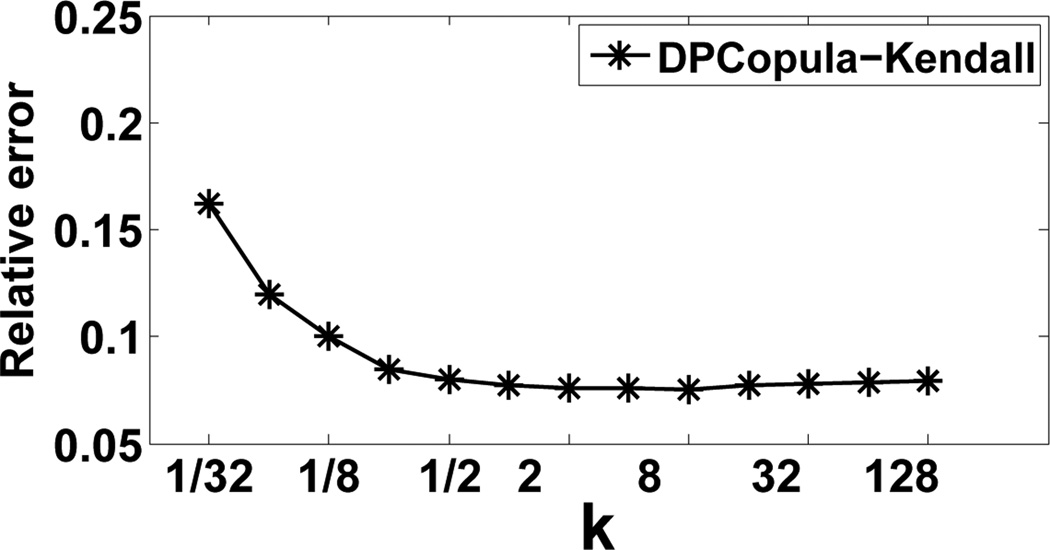
Since k is the only algorithmic parameter in the DPCopula method, we first evaluate its impact on the effectiveness of the method. Figure 5 shows the relative error of DPCopula-Kendall method for random count queries with respect to varying k for 2D synthetic data. DPCopula-MLE has similar trends and we omit it for the clarity of the graph. We observe that when k is less than 1, the relative error clearly degrades as k increases. When k is greater than 1, the relative error does not change significantly. This shows that having a higher budget allocated for computing differentially private margins than the coefficients ensures better query accuracy. In addition, the method is quite robust and insensitive to the value of k as long as it is greater than 1, which alleviates the burden of parameter selection on the users. For the remaining experiments, we set the value of k to 8.

Figure 5.

Relative error vs. Ratio k

DPCopula-MLE vs. DPCopula-Kendall

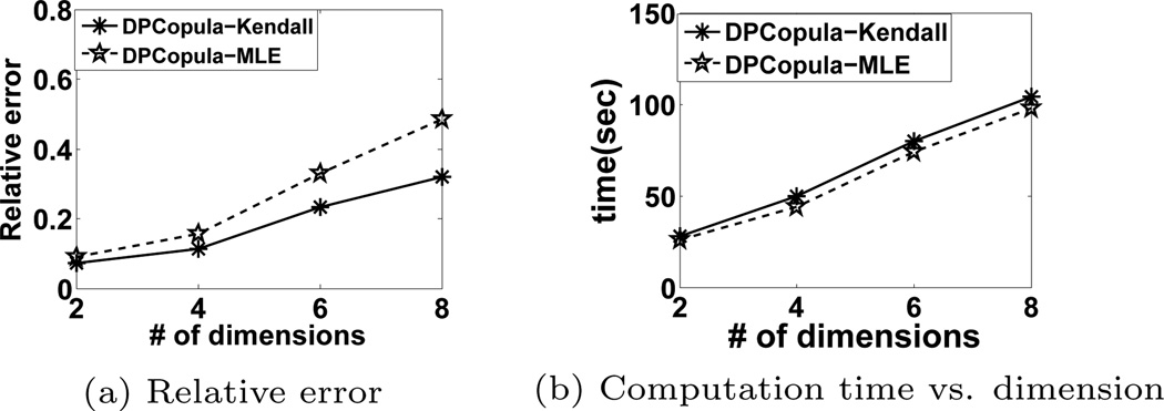
Figure 6 investigates the trade-off between two DPCopula methods. Figure 6(a) compares the relative error for random queries of the two methods on synthetic data with varying number of dimensions and n = 10⁶ considering the sensitivity of DPCopula-MLE. We observe that DPCopula-Kendall performs better than DPCopula-MLE. This is because the sensitivity of the general coefficient in DPCopula-MLE is higher than DPCopula-Kendall. As a consequence, the correlation matrix estimated by DPCopula-Kendall is more accurate than DPCopula-MLE. Figure 6(b) shows the runtime of the two methods. We can see that with higher dimensions, the time to compute the coefficients becomes longer because the time complexity of DPCopula is quadratic with the number of dimensions. We use the sampling method in all experiments to reduce the computation time. DPCopula-Kendall has a slightly higher computation overhead than DPCopula-MLE while the total computation time for both methods are quite efficient. We show that the computation time of DPCopula is acceptable for various data cardinalities and dimensions in later experiments. In the remaining experiments, we only use DPCopula-Kendall to compare with other methods.

Figure 6.

DPCopula-Kendall vs. DPCopula-MLE

5.3 Comparison on real datasets

Query accuracy vs. differential privacy budget

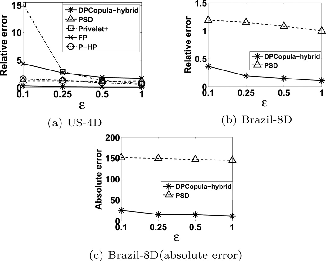
Figure 7 compares DPCopula with other methods with respect to varying differential privacy budget. Figure 7(a)–(b) shows the relative error for random range count queries on the US census dataset and Brazil dataset, respectively. Note that we use DPCopula-hybrid on top of DPCopula-Kendall for both datasets since they contain binary attributes. From both figures, we observe that DPCopula outperforms all the other methods and their performance gap expands as the privacy budget decreases. The noise incurred by partitioning small domain attributes imposes little impact on the performance of DPCopula. In addition, the accuracy of DPCopula is robust against various epsilon values. This overall good performance is due to the fact that DPCopula method only computes DP margins and DP correlation matrix whose inuence on the accuracy is much smaller than the margins. Meanwhile, the other methods require noise being added to histogram cells or partitions and introduce either large perturbation errors or estimation errors.

Figure 7.

Relative error vs. differential privacy budget

5.4 Comparison on synthetic datasets

We use synthetic datasets to evaluate the impact of query range size, distributions of each dimension, and dimensionality on the error, since we can vary these parameters easily in synthetic data.

Query accuracy vs. query range size

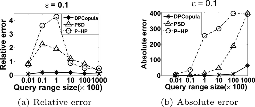
We study the impact of query range size on the query accuracy for different methods. For each query range size, we randomly generated queries such that the product of the query ranges on each dimension is the same. We use 2D synthetic data in order to include P-HP. We set the privacy budget ε to be 0.1 to better present the performance difference of three methods. The trend is similar for PSD and DPCopula in higher dimension data. Figure 8 presents the impact of various query range sizes on the query accuracy in terms of relative error and absolute error. DPCopula outperforms PSD and P-HP. For all methods, the relative error gradually degrades as the query range size increases while the absolute error has the contrary trend. The reason is that when the query size is small, the true answer A_act(q) is also small which may incur a small absolute error but large relative error. For the cell-based query (i.e. query range size is 1), the average relative error is small because the relative errors of most cell-based queries are zeros, which greatly reduces the average value.

Figure 8.

Query accuracy vs. query range size

Relative error vs. distribution

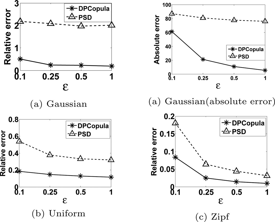
Figure 9 presents the relative error for 8D data with Gaussian dependence and all margins respectively generated from the Gaussian distribution, uniform distribution and zipf distribution, under various ε values. Akin to the results in Figure 7, DPCopula performs best in all distributions, and significantly outperforms PSD especially when the margin is skewed. Meanwhile, this verifies that DPCopula using Gaussian copula performs well not only for data with Gaussian distributions but also for data with different marginal distributions as long as they follow the Gaussian dependence. An interesting phenomenon is that DPCopula performs better on the uniform and zipf data than Gaussian distribution data. This is because the method used for generating marginal DP histograms in DPCopula, EFPA, performs better on uniform-distributed data than skewed data.

Figure 9.

Relative error vs. distribution

Query accuracy vs. dimensionality

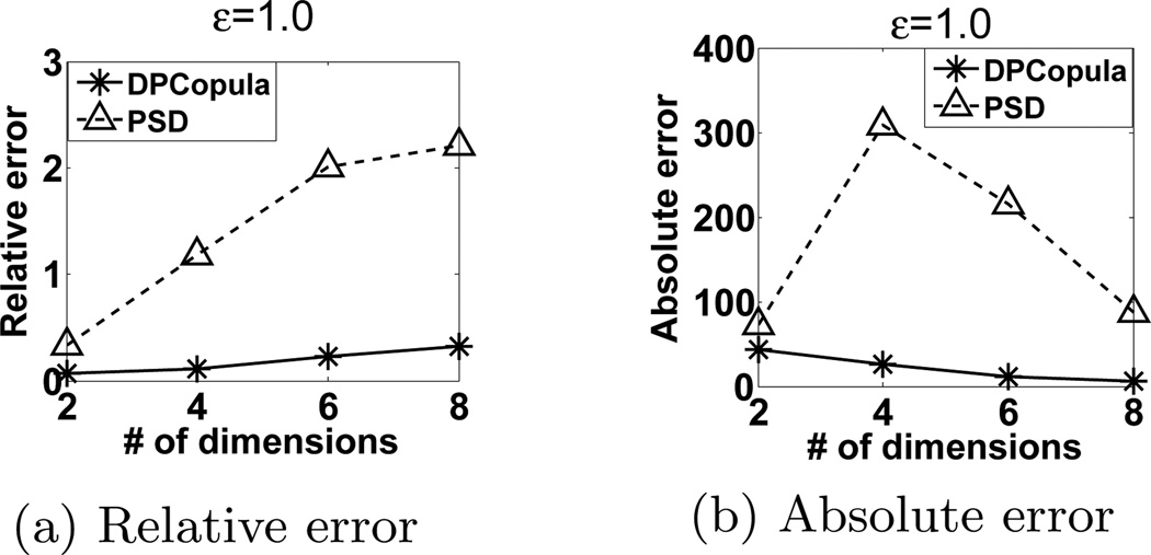
We study the effect of the dataset dimensionality as shown in Figure 10. All marginal distributions of synthetic datasets in various dimensions are Gaussian distribution with domain size of 1000. We set the dimensionality ranging from 2D to 8D which corresponds to domain space of 10⁶ to 10²⁴. So the dataset is highly sparse with only 50000 records. For all dimensions from 2D to 8D, DPCopula again outperforms PSD. The 2D data has the lowest relative error and absolute error for both methods. The query accuracy of all methods from 4D to 8D gradually drops with the performance gap gradually expanding as the number of dimensions increases. For DPCopula, this is due to the fact that for a fixed overall privacy budget ε, higher dimensionality means less privacy budget is allocated to each margin and correlation coefficient incurring larger amount of noise. For PSD, consistent with the analysis in [9], higher dimensionality will increase the size of the domain space ${\prod }_{i=1}^m|A_i|$, resulting in larger relative error. We can also observe that the increasing relative errors for DPCopula are incurred by the small true answers with higher dimensions.

Figure 10.

Query accuracy vs. dimensionality

Scalability

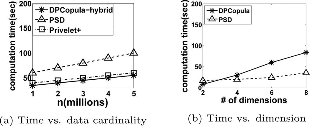
Figure 11(a) illustrates the computation time with various data cardinality n using the 4D US census dataset. Observe that all three techniques run linear time with respect to n. Computing the correlation matrix is not a bottleneck for DPCopula as we use the sampling technique. PSD incurs a higher computation overhead than DPCopula and Privelet+ since its time complexity O(mn̂logn̂) is linearithmic with n̂, where n̂ = 0.01 × n. Figure 11(b) illustrates the computation time with various dimensions and data cardinality fixed to 50000. DPCopula has a higher computation overhead than PSD because the time complexity is quadratic with the number of dimensions but the time for 8D is still quite acceptable. In contrast, all the other methods including EPFA that use histograms as input are not shown here due to their high time and space complexity due to the large domain sizes.

Figure 11.

Time efficiency

6. CONCLUSIONS

In this paper, we presented DPCopula using copula functions for differentially private multi-dimensional data synthesization. Different from existing methods, DPcopula captures marginal distribution of each dimension and dependence between separate dimensions via copula functions. Our experimental studies on various types of datasets validated our theoretical results and demonstrated the efficiency and effectiveness of our algorithm, particularly on high-dimensional and large domain datasets.

In the future, we plan to extend our research on the following directions. First, we are interested in employing other copula families and investigate how to select optimal copula functions for a given dataset. Second, we are interested in developing data synthesization mechanisms for dynamically evolving datasets.

REFERENCES

- 1.Ács G, Castelluccia C, Chen R. Differentially private histogram publishing through lossy compression. ICDM. 2012 [Google Scholar]
- 2.Barak B, Chaudhuri K, Dwork C, Kale S, McSherry F, Talwar K. Privacy, accuracy, and consistency too: a holistic solution to contingency table release. PODS. 2007 [Google Scholar]
- 3.Benjamin RC, Fung CM, Wang Ke, Yu PS. Privacy-preserving data publishing: A survey of recent developments, ACM Computing Surveys. 2010 [Google Scholar]
- 4.Bluhm, C OL, Wagner C. An introduction to credit risk modeling. Chapman and Hall, Boca Raton [Google Scholar]
- 5.Blum A, Ligett K, Roth A. A learning theory approach to non-interactive database privacy. STOC. 2008:609–617. [Google Scholar]
- 6.Bouye, E VDANGR, Roncalli T. Copulas for finance a reading guide and some applications. 2000 [Google Scholar]
- 7.Burridge J. Information preserving statistical obfuscation. Statistics and Computing. 2003;13(4):321–327. [Google Scholar]
- 8.Chen S, Zhou S, Bhowmick SS. Integrating historical noisy answers for improving data utility under differential privacy. EDBT. 2012:62–73. [Google Scholar]
- 9.Cormode G, Procopiuc CM, Srivastava D, Shen E, Yu T. Differentially private spatial decompositions. ICDE. 2012 [Google Scholar]
- 10.Cormode G, Procopiuc CM, Srivastava D, Tran TTL. Differentially private summaries for sparse data. ICDT. 2012:299–311. [Google Scholar]
- 11.Demarta S, McNeil AJ. The t copula and related copulas. International Statistical Review. 2007;73:111–129. [Google Scholar]
- 12.Ding B, Winslett M, Han J, Li Z. Differentially private data cubes: optimizing noise sources and consistency; SIGMOD Conference; 2011. [Google Scholar]
- 13.Dwork C. Differential privacy. Automata, Languages and Programming, Pt 2. 2006:4052. [Google Scholar]
- 14.Dwork C. Differential privacy: A survey of results. In: Agrawal M, Du D-Z, Duan Z, Li A, editors. TAMC, volume 4978 of Lecture Notes in Computer Science. Springer; 2008. pp. 1–19. [Google Scholar]
- 15.Dwork C. A firm foundation for private data analysis. Commun. ACM. 2011 [Google Scholar]
- 16.Dwork C, Mcsherry F, Nissim K, Smith A. Calibrating Noise to Sensitivity in Private Data Analysis. Theory of Cryptography. :1–20. [Google Scholar]
- 17.Dwork C, Smith A. Differential privacy for statistics: What we know and what we want to learn. Journal of Privacy and Confidentiality. 2009;1(Number 2):135–154. [Google Scholar]
- 18.Friedman A, Schuster A. Data mining with differential privacy. SIGKDD. 2010 [Google Scholar]
- 19.Hayy M, Rastogiz V, Miklauy G, Suciu D. Boosting the accuracy of Differentially-private histograms through consistency. VLDB. 2010 [Google Scholar]
- 20.Joe H. Multivariate models and dependence concepts. Chapman and Hall, New York. 1997 [Google Scholar]
- 21.Reiter J. disclosure limitation in longitudinal linked data. Confidentiality, Disclosure, and Data Access: Theory and Practical Applications for Statistical Agencies. 2001:215–277. [Google Scholar]
- 22.Kifer D, Machanavajjhala A. No free lunch in data privacy; Proceedings of the 2011 international conference on Management of data, SIGMOD ’11; 2011. [Google Scholar]
- 23.Li C, Hay M, Rastogi V, Miklau G, McGregor A. Optimizing linear counting queries under differential privacy. PODS. 2010:123–134. [Google Scholar]
- 24.Li D. On default correlation: a copula function approach. Journal of Fixed Income. 2000;9:43–54. [Google Scholar]
- 25.Lindner A, Szimayer A. A limit theorem for copulas. 2003 Dwonload from www-m4.ma.tum.de/m4/pers/lindner. [Google Scholar]
- 26.Liu H, Han F, Yuan M, Lafferty JD, Wasserman LA. High dimensional semiparametric gaussian copula graphical models. ICML. 2012 [Google Scholar]
- 27.Machanavajjhala A, Kifer D, Abowd J, Gehrke J, Vilhuber L. Privacy: Theory meets practice on the map. ICDE. 2008 [Google Scholar]
- 28.McSherry . SIGMOD. New York, NY, USA: ACM; 2009. Privacy integrated queries: an extensible platform for privacy-preserving data analysis. [Google Scholar]
- 29.McSherry F, Talwar K. Mechanism design via differential privacy. FOCS. 2007:94–103. [Google Scholar]
- 30.Mohammed N, Chen R, Fung BCM, Yu PS. Differentially private data release for data mining. SIGKDD. 2011 [Google Scholar]
- 31.Nelsen RB. An Introduction to Copulas. Springer; 1999. [Google Scholar]
- 32.Osband K. Iceberg Risk: An Adventure in Portfolio Theory. 2002 [Google Scholar]
- 33.Qardaji WH, Yang W, Li N. Differentially private grids for geospatial data. ICDE. 2013 [Google Scholar]
- 34.Rosenberg J. Npon-parametric pricing of multivariate contingent claims. Journal of Derivatives. 2003;10:9–26. [Google Scholar]
- 35.Rousseeuw G. Peter ; Molenberghs. Transformation of non positive semidefinite correlations matrices. Communications in statistics: theory and methods. 1993;22:965–984. [Google Scholar]
- 36.Sklar A. Fonctions de rĺępartition ĺd’ n dimensions et leurs marges. Publications de l’Institut de statistique de l’Universitĺę de Paris. 1959;8:229–231. [Google Scholar]
- 37.Wasserman L, Zhou S. A statistical framework for differential privacy. JASA. 2009;105(489):375–389. [Google Scholar]
- 38.Xiao X, Tao Y. Output perturbation with query relaxation. VLDB. 2008 [Google Scholar]
- 39.Xiao X, Wang G, Gehrke J. Differential privacy via wavelet transforms. ICDE. 2010:225–236. [Google Scholar]
- 40.Xiao Y, Gardner JJ, Xiong L. Dpcube: Releasing Differentially private data cubes for health information. ICDE. 2012 [Google Scholar]
- 41.Xu J, Zhang Z, Xiao X, Yang Y, Yu G. Differentially private histogram publication. ICDE. 2012 [Google Scholar]
- 42.Yaroslavtsev G, Cormode G, Procopiuc CM, Srivastava D. Accurate and efficient private release of datacubes and contingency tables. ICDE. 2013 [Google Scholar]
- 43.Yuan G, Zhang Z, Winslett M, Xiao X, Yang Y, Hao Z. Low-rank mechanism: Optimizing batch queries under differential privacy. PVLDB. 2012;5(11):1352–1363. [Google Scholar]