Abstract
In classical growth analysis, relative growth rate (RGR) is calculated as RGR = (ln W2 – ln W1)/(t2 – t1), where W1 and W2 are plant dry weights at times t1 and t2. Since RGR is usually calculated using destructive harvests of several individuals, an obvious approach is to substitute W1 and W2 with sample means 1 and 2. Here we demonstrate that this approach yields a biased estimate of RGR whenever the variance of the natural logarithm‐transformed plant weight changes through time. This bias increases with an increase in the variance in RGR, in the length of the interval between harvests, or in sample size. The bias can be avoided by using the formula  , where
  and
and  are the means of the natural logarithm‐transformed plant weights.
Key words: Relative growth rate, growth analysis, methodology, bias
INTRODUCTION
Growth analysis is a widely used analytical tool for characterizing plant growth. Of the parameters typically calculated, the most important is relative growth rate (RGR), defined as the parameter r in the equation:

where W1 and W2 are plant dry weights at times t1 and t2. Rearrangement of terms yields the equation used to calculate RGR in what is called the classical approach (Hunt, 1982):

Since eqn (1) describes the growth of a single individual, eqn (2) provides a formula for calculating the RGR of a single individual. Destructive harvesting is required to determine plant dry weight, so in practice RGR is calculated from samples of individuals from the same cohort at two points in time (Evans, 1972). While eqn (2) is widely presented in studies utilizing classical growth analysis, it has generally been overlooked that this formula does not provide an unequivocal interpretation of how RGR should be calculated. Several possible interpretations of eqn (2) arise when calculating RGR from samples of individuals. The first, and most obvious, approach is to simply substitute W1 and W2 with sample means 1 and 2, estimating RGR as:

Hereafter, we will refer to this as estimator 1.
Alternatively, RGR can be calculated from the mean natural logarithm‐transformed plant weights:

where  is the mean of the ln‐transformed plant weights at time t. We will refer to this as estimator 2. In the first estimator, plant weights are averaged before ln‐transforming, whereas in the second estimator, the weights are ln‐transformed before averaging. These estimators almost always yield different values due to the fact that ln () is not equal to
  if there is variation in plant weight among individuals (Aitchison and Brown, 1976).
Additionally, RGR can be calculated using the pairing method or the functional approach. In the pairing method (Evans, 1972), plants are grouped into pairs of similarly sized individuals before the first harvest. One plant of each pair is harvested on the first harvest date, and the other plant is harvested on the second date. RGR is then calculated for each pair, and the values averaged over all pairs. We show in the Appendix that the estimate provided by this approach is identical to that of estimator 2. Alternatively, in the functional approach, a curve is fit to the ln‐transformed plant weights through time and RGR at a particular time is calculated as the slope of the curve. When applied to harvests made at only two points in time, the results are identical to estimator 2. While these two methods offer the advantage of providing estimates of the variance in RGR, we do not consider either of these further because the estimates of RGR do not differ from estimator 2.
As far as we know, little attention has been given to the fact that two interpretations of eqn (2) do exist, and that they might yield different estimates of RGR. As a consequence, recommendations vary among authors as to which estimator should be used. For example, McGraw and Garbutt (1990) recommend the first approach, Venus and Causton (1979) and Causton and Venus (1981) recommend the second, and Radford (1967) and Evans (1972)suggest the pairing method. Other texts offer no insight as to which form to use (Hunt, 1982, 1990; Chiariello et al., 1991).
In most research reports there has been a similar lack of attention to this issue. Examining issues of Annals of Botany from 1993 to 2001, we identified 28 papers applying classical growth analysis. Of these, one utilized estimator 1, five used estimator 2 and in the remaining 22 studies it was not possible to infer which equation was used. Clearly, this is an aspect that has not received enough attention. Therefore, in this paper, we analyse the performance of these two estimators to permit well‐founded recommendations for the correct choice of estimator.
MATERIALS AND METHODS
To determine if these two estimators yield unbiased estimates of RGR, i.e. that their expected values are identical to the true mean RGR, we attempted to derive analytically the expected values of the two estimators. While this analytical approach was possible for the second estimator, for the first it was necessary to resort to a second‐order approximation of the expected value.
Since we were unable to find an exact form for the expected value of both equations, we relied on simulations to substantiate the differences between these estimators and to confirm the generality of the results. In the first set of simulations we generated data corresponding to a typical experiment in which ten individuals were harvested on each of two dates. Since plant weight is commonly lognormally distributed (Poorter and Garnier, 1996), we used this distribution in our simulations. To generate an individual plant weight, the algorithm of Press et al. (1989) was used to generate a ln W value from a normal distribution. This value was then transformed with the exponential function to arrive at W. The variance of the underlying normal distribution is σ2ln W, which is the variance of the ln‐transformed plant weights.
Since it is variation in plant weight that causes the two estimators to yield different estimates of RGR, we examined the effect of the variances σ2ln W1, σ2ln W2 as well as RGR on possible bias in the RGR estimates. Using an initial true mean weight (W1) of 1 g and a harvest interval of 50 d, we generated cases in which we varied σ2ln W1, σ2ln W2 and the true mean RGR independently of each other. We used a fully factorial array of cases using six levels of RGR (0·05, 0·10, 0·15, 0·20, 0·25, 0·30 g g–1 d–1) and eight levels each of σln W1 and σln W2 (0·1, 0·2, 0·3, 0·4, 0·5, 0·6, 0·7, 0·8). For each combination of parameters, 10 000 simulations were run. For each simulation, RGR was calculated from the generated data using both estimators and results were compared with the true mean RGR.
In a second set of simulations, we examined the effects of increasing variance in RGR, time between harvests and sample size on the performance of these two estimators. In these simulations, plant weights (W1) for the initial harvest were randomly generated from a lognormal distribution. Plant weights for the second harvest were generated as W2 = W′1ert}, where r was generated from a normal distribution with a mean of 0·05 g g–1 d1. For these latter weights, W′1 was generated from the same probability distribution as the W1 of the first harvest. Here we distinguish between W1 and W′1 to simulate a realistic case in which different individuals are sampled on the two harvest dates. The term W1 denotes the weight at time 1 of individuals that were harvested at time 1, whereas W′1 is the weight at time 1 of individuals that were harvested at time 2. Cases were run for a range of values of σRGR from 0 to 0·03, a range of harvest intervals from 5 to 200 d, and a range of sample sizes from one to 40 individuals per harvest. For each set of conditions tested, 10 000 simulations were run.
In the above simulations, we assumed that plant weight is lognormally distributed and that RGR is normally distributed, so we ran a third set of simulations to test whether the performance of the two estimators depends on the probability distributions used to generate plant weight and RGR. It is not feasible to examine all possible probability distributions, so we limited our study to the normal, lognormal and exponential distributions. Normal and exponential distributions were chosen to provide cases that are either unskewed or more strongly right‐skewed than the lognormal distribution. Probability distributions were generated using the algorithms of Press et al. (1989).
RESULTS AND DISCUSSION
In agreement with Causton and Venus (1981), we demonstrate that estimator 2 is unbiased; i.e. the expected value of this estimator (2) is equal to the true mean RGR. In contrast, estimator 1 is biased. As shown in the Appendix, when plant weight is lognormally distributed, the bias is approximately equal to:

where n is the number of individuals sampled per harvest date and ρ is the true mean RGR. A lognormal distribution in plant weight develops naturally when RGR or germination time is normally distributed (Poorter and Garnier, 1996), so the assumption of lognormality is probably appropriate in most applications.
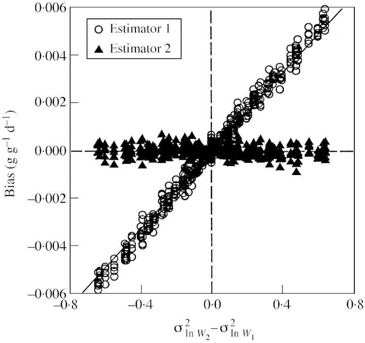
In the first set of simulations, where σ2ln W1, σ2ln W2 and mean RGR were varied independently of each other, we confirm that the first estimator is biased but the second is not (Fig. 1). The size of the bias depends on the values of plant variability. If σ2ln W remains constant through time, the bias is nil, but the larger the difference between σ2ln W1 and σ2ln W2, the larger the error. Consequently, the relationship between (σ2ln W2 – σ2ln W1 and the bias is well described by a single curve, regardless of the value of RGR. The approximate bias, as estimated by eqn (5), closely fits the simulated values (Fig. 1).
Fig. 1. Relationship between the difference in variance at two harvest times and simulated bias of the two RGR estimators. Results are from a fully factorial array of simulations using six levels of RGR (0·05, 0·10, 0·15, 0·20, 0·25, 0·30 g g–1 d–1) and eight levels each of and (0·1, 0·2, 0·3, 0·4, 0·5, 0·6, 0·7, 0·8). Each point represents the mean of 10 000 simulations with a sample size of ten individuals in each harvest. The continuous line shows the bias as estimated by eqn (5).
A change in σ2ln W through time can occur only if there is some variation in RGR among individuals, so it is useful to examine how variation in RGR affects the bias of the first estimator (2). By applying rules for variances of linear combinations of variables to eqn (1), it can be shown that when RGR and W1 are independent of each other then

Therefore, the bias of the first estimator is expected to increase in response to increased time between harvests or increased variance in RGR, as confirmed by the second set of simulations (Fig. 2A and B). These simulations also demonstrate that the bias increases with increasing sample size, as to be expected from eqn (5) (Fig. 2C).
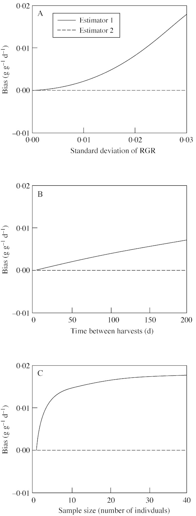
Fig. 2. Simulation results demonstrating the effect of variation in RGR (A), time between harvests (B) and sample size (C) on the bias of the two RGR estimators. In A, RGR was fixed at 0·05, with a harvest interval of 50 d and a harvest size of ten individuals. In B, RGR was fixed at 0·05 with a standard deviation of 0·01 and a sample size of ten individuals. In C, RGR was fixed at 0·05 with a standard deviation of 0·02 and harvest interval of 100 d. For each set of parameters, 10 000 simulations were run.
In general, if there is any variation in RGR among individual plants, σ2ln W2will be larger than σ2ln W1, and estimator 1 will have a positive bias, provided that RGR and W1 are independent variables. In reality, RGR and W1 need not be independent of each other. We might expect a negative covariance between RGR and W1 due to the frequently observed decline in RGR through plant development. If larger plants at t1 are those individuals that have reached a more advanced stage of development, they may subsequently exhibit lower growth rates than smaller individuals. Such a decline could be due to developmental changes in allocation or photosynthesis, or could arise from an increasingly limiting nutrient supply. Similarly, there is often a negative correlation between seed size and RGR, at least among species (Swanborough and Westoby, 1996). If a similar relationship occurs within a species, a negative covariance between W1 and RGR could emerge. In any case, a negative correlation between W1 and RGR would reduce the tendency of σ2ln W to increase through time and thereby reduce the bias of estimator 1. If this negative covariance is large enough, it could result in a decline in σ2ln W through time, causing a negative bias, as appears in Fig. 1.
In contrast, there could be a positive correlation between W1 and RGR due to genetic variation in RGR, whereby plants attaining higher W1 due to higher RGR continue growing at a greater RGR. Alternatively, in experimental situations permitting competition among individuals, larger individuals may gain a competitive advantage and therefore maintain higher RGR than competitively suppressed individuals. Either of these situations could result in a positive covariance between W1 and RGR, thereby accentuating the quantity σ2ln W2 – σ2ln W1 and consequently the bias of estimator 1.
How important is the bias in RGR when using the wrong estimator? We used experimental data to demonstrate that the bias can be large enough to be of concern. In a study involving 18 tree and shrub species from the cerrado savannas of Brazil (W.A. Hoffmann, unpubl. res.), mean sample variance, s2ln W, increased from 0·17 at 50 d to 0·18 at 100 d and to 0·27 at 150 d. We estimated the bias of the calculated RGR for each species using eqn (5). On average, the bias was estimated to be +1 % and +13 % for the first and second intervals, respectively, demonstrating that the bias is substantial.
With experimental data, we cannot know the true bias since we must rely on s2ln W, which is an estimate of the true σ2ln W based on finite samples. Similarly, we must depend on a second‐order approximation of the bias. The simulations indicate that this approximation provides a reliable estimate of bias, at least for reasonable values of σ2ln W1 and σ2ln W2.
Another uncertainty with experimental data is that plant weight may not be lognormally distributed. However, the third set of simulations indicates that this bias is not limited to lognormally distributed data. Regardless of the probability distribution used to generate plant weight and RGR, estimator 1 was biased whereas estimator 2 was not (Table 1).
Table 1.
. Simulation results using different probability distributions for initial weight and variance of RGR
| Initial weight distribution | Initial plant weight (g) (mean + s.d.) | RGR distribution | RGR (g g–1 d–1) (mean + s.d.) | Bias of estimator 1 (g g–1 d–1) | Bias of estimator 2 (g g–1 d–1) |
| Normal | 1 (0·2) | Normal | 0·05 (0·01) | 0·0043 | 0·0000 |
| Normal | 1 (0·2) | Lognormal | 0·05 (0·01) | 0·0024 | 0·0000 |
| Normal | 1 (0·2) | Exponential | 0·05 (0·05) | 0·0753 | 0·0000 |
| Lognormal | 1 (0·2) | Normal | 0·05 (0·01) | 0·0022 | 0·0000 |
| Lognormal | 1 (0·2) | Lognormal | 0·05 (0·01) | 0·0024 | 0·0000 |
| Lognormal | 1 (0·2) | Exponential | 0·05 (0·05) | 0·0583 | 0·0001 |
| Exponential | 1 (1) | Normal | 0·05 (0·01) | 0·0038 | 0·0000 |
| Exponential | 1 (1) | Lognormal | 0·05 (0·01) | 0·0023 | 0·0002 |
| Exponential | 1 (1) | Exponential | 0·05 (0·05) | 0·0708 | 0·0007 |
Simulations were run for 100 d, with mean initial weight of 1 g and mean RGR of 0·050 g g–1 d–1. Note that for an exponential distribution, the standard deviation is constrained to be equal to the mean, so when this distribution is used, it was not possible to utilize the same standard deviation as was used for the others.
In conclusion, estimator 1 presented in eqn (3) is biased and should therefore be avoided in RGR calculations. We suggest the use of estimator 2, as given in eqn (4), exclusively, as this equation yields an unbiased estimate of RGR under all conditions.
ACKNOWLEDGEMENTS
We thank Feike Schieving for checking the mathematical derivations and Danny Tholen, Rens Voesenek, Adrie van der Werf and Kaoru Kitajima for comments on the manuscript.
APPENDIX
Proof that the pairing method is equivalent to estimator 2
Here we demonstrate that the pairing method (Evans, 1972) is equivalent to the second estimator [eqn (4)]. In the pairing method, plants are grouped into pairs of similarly sized plants. One plant of each pair is harvested at time t1, and the other at time t2. RGR is then calculated for each pair j, and then these values are subsequently averaged over all pairs. RGR is therefore estimated as:

where n is the number of pairs and Wij is the dry weight of individual j of harvest i.
This reduces as follows:
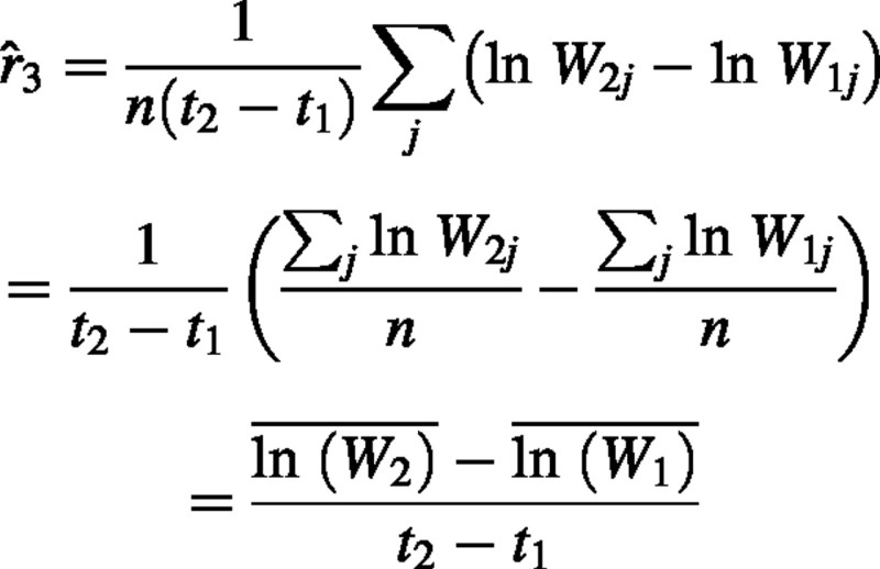
This is therefore equivalent to eqn (4).
Proof that 2 is an unbiased estimator of RGR
Here we demonstrate that

is an unbiased estimator of RGR. The weight at time 2 of an individual i can be expressed as  , where t2 – t1 is replaced with Δt. The estimator can now be rewritten as

We distinguish between W1 and W′1 because different individuals are sampled on the two harvest dates. The term W1 denotes the weight at time 1 of individuals that were harvested at time 1, whereas W′1 is the weight at time 1 of the individuals that were harvested at time 2. We assume that the individuals harvested at the two times are chosen randomly from the same cohort, so W1 and W′1 are identically distributed random variables.
Using theorems for linear combinations of random variables (Rice, 1988; pp. 109–112), the expected value of is:
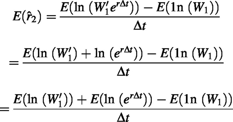
Since W1 and W′1 are identically distributed random variables, their expected values are identical. Therefore  ρ where ρ, is the true mean RGR. Since the expected value of the estimator 2 is equal to the expected value of RGR, we can conclude that 2 is an unbiased estimator.
Proof that 1 is a biased estimator of RGR
Here we demonstrate that  is a biased estimator of RGR. The expected value of this estimator is

We were unable to derive an exact solution for this estimator so we used the second‐order approximation:

(Rice, 1988; p. 143), where μw is the true population mean plant dry weight and 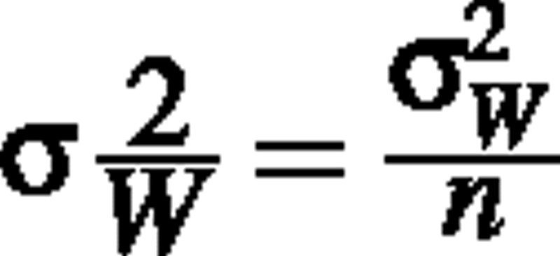 is the true variance of the mean of plant dry weight, based on some sample size n. If W is lognormally distributed, we know that

and

(Aitchison and Brown, 1976), so

and
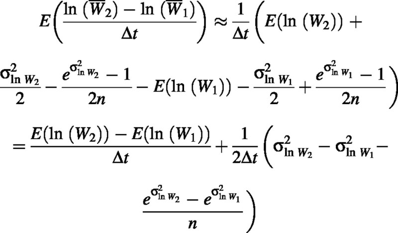
The first term of the right‐hand side of this equation is the expected value of RGR, so the bias is approximately

Supplementary Material
Received: 3 December 2001; Returned for revision: 22 February 2002; Accepted: 14 March 2002
References
- AitchisonJ, Brown JAC.1976. The lognormal distribution. Cambridge: Cambridge University Press. [Google Scholar]
- CaustonDR, Venus JC.1981. The biometry of plant growth. London: Edward Arnold. [Google Scholar]
- ChiarielloNR, Mooney HA, Williams K.1991. Growth, carbon allocation and cost of plant tissues. In: Pearcy RW, Ehleringer J, Mooney HA, Rundel PW, eds. Plant physiological ecology London: Chapman and Hall, 327–366. [Google Scholar]
- EvansGC.1972. The quantitative analysis of plant growth. Oxford: Blackwell Scientific. [Google Scholar]
- HuntR.1982. Plant growth curves. London: Edward Arnold. [Google Scholar]
- HuntR.1990. Basic growth analysis: plant growth analysis for beginners. London: Unwin Hyman. [Google Scholar]
- McGrawJB, Garbutt K.1990. Demographic growth Analysis. Ecology 71: 1199–2004. [Google Scholar]
- PoorterH, Garnier E.1996. Plant growth analysis: an evaluation of experimental design and computational methods. Journal of Experimental Botany 47: 1343–1351. [Google Scholar]
- PressWH, Flannery BP, Teukolsky SA, Vetterling WT.1989. Numerical recipes in Pascal. Cambridge: Cambridge University Press. [Google Scholar]
- RadfordPJ.1967. Growth analysis formulae – their use and abuse. Crop Science 7: 171–175 [Google Scholar]
- RiceJA.1988. Mathematical statisitcs and data analysis. Patricia Grove: Wadsworth and Brooks/Cole. [Google Scholar]
- SwanboroughP, Westoby M.1996. Seedling relative growth rate and its components in relation to seed size: phylogenetically independent contrasts. Functional Ecology 10: 176–184. [Google Scholar]
- VenusJC, Causton DR.1979. Plant growth analysis: a re‐examination of the methods of calculation of relative growth and net assimilation rates without using fitted functions. Annals of Botany 43: 633–638. [Google Scholar]
Associated Data
This section collects any data citations, data availability statements, or supplementary materials included in this article.


