Instantaneous Canopy Photosynthesis: Analytical Expressions for Sun and Shade Leaves Based on Exponential Light Decay Down the Canopy and an Acclimated Non‐rectangular Hyperbola for Leaf Photosynthesis

Abstract

Analytical expressions for the contributions of sun and shade leaves to instantaneous canopy photosynthesis are derived. The analysis is based on four assumptions. First, that the canopy is closed in the sense that it is horizontally uniform. Secondly, that there is an exponential profile of light down the canopy with the same decay constant for light from different parts of the sky. Thirdly, that the leaf photosynthetic response to incident irradiance can be described by a three‐parameter non‐rectangular hyperbola (NRH). And lastly, that light acclimation at the leaf level occurs in only one parameter of the NRH, that describing the light‐saturated photosynthetic rate, which is assumed to be proportional to the local averaged leaf irradiance. These assumptions have been extensively researched empirically and theoretically and their limitations are quite well understood. They have been widely used when appropriate. Combining these four assumptions permits the derivation of algebraic expressions for instantaneous canopy photosynthesis which are computationally efficient because they avoid the necessity for numerical integration down the canopy. These are valuable for modelling plant and crop ecosystems, for which canopy photosynthesis is the primary driver. Ignoring the sun/shade dichotomy can result in overestimates of canopy photosynthesis of up to 20 %, but using a rectangular hyperbola instead of a non‐rectangular hyperbola to estimate canopy photosynthesis taking account of sun and shade leaves can lead to a similarly sized underestimate.

INTRODUCTION

Canopy photosynthesis is the primary driver for models of crop growth and plant ecosystems. It has therefore remained a topic of much continuing research, development and application. Canopy photosynthesis presents two difficulties to the modeller of plant ecosystems. These are both concerned with integration: over time and over space. These difficulties are sometimes described, possibly misleadingly, as ‘scaling’ problems (cf. Enquist et al., 1998). Ecosystem models are usually quite large and often need to be run over 100s of simulated years. Execution time is always far greater than the modeller would wish. To be more specific, if it is possible to run the model with a daily time step instead of one of 10 min, or, if it is possible to avoid numerical integration down the crop canopy and perhaps down the soil profile, then these are valuable gains. However, they must be achievable without too much loss of realism, for necessarily they involve approximation. Nevertheless, it must be stressed that ‘acceptable realism’ depends on objectives as well as situations. Foresters, grassland ecologists and crop scientists have different perspectives. It may not be wise to attempt to build a model that works equally well in Scotland and in Australia, although this is not to doubt the similarity of the underlying mechanisms. It is now generally accepted that, below‐ground, explicit spatial integration is frequently, but not always, required. A recent example of such a model is that by Chertov et al. (2001). Restricting ourselves to canopy photosynthesis, first temporal and then spatial aspects are reviewed.

Recently Sands (1995) derived equations for daily canopy photosynthesis assuming exponential light decay down the canopy (Monsi and Saeki, 1953), a non‐rectangular hyperbola for leaf photosynthesis (Rabinowitch, 1951; Chartier, 1966), a daily sinusoid for above‐canopy photosynthetically active radiation (PAR) and that the acclimated P_max (light‐saturated leaf photosynthetic rate) for a leaf within the canopy is proportional to the ratio of PAR at that position to PAR above the canopy. The last two assumptions were proposed by Charles‐Edwards (1981, 1982). Sands’ (1995) equations are useful for modellers who wish to use a daily time step and who are prepared to neglect diurnal effects; Sands also ignores the different contributions of sun and shade leaves which may be important under certain conditions due to the non‐linearity of leaf response to light. Important diurnal effects may be stomatal closure during the daylight hours, and variations in sugar concentrations and water‐related variables. Many crop and ecosystem modellers believe it essential to represent these diurnal changes explicitly and therefore use a time step of an hour or less (de Wit et al., 1970; Thornley, 1998a).

The leaf/canopy spatial integration problem has been reviewed by Amthor (1994). Sinclair and Horie (1989) described a simplifed sun–shade canopy model using a two‐parameter negative exponential leaf light response, apparently summed numerically down the canopy. They concluded that their simple model gave results within 12 % of a far more complex model, treating 15 horizons each with 20 leaf classes. Medlyn et al. (2000, Appendix) derived analytical expressions for canopy photosynthesis based on exponential light decay down the canopy (Monsi and Saeki, 1953), acclimation essentially according to Charles‐Edwards (1981, 1982), treating sun and shade contributions separately, but using a rectangular hyperbola for leaf light response. The reason for separate calculation of sun and shade contributions is to allow for the non‐linearity of the leaf response to light. With two‐parameter equations such as the rectangular hyperbola or the negative exponential, the two parameters denote the initial slope and the asymptote, and there is no parameter to adjust the non‐linearity in the all‐important central region of the response. The extra parameter of the non‐rectangular hyperbola is the reason for its empirical success (see below), and its importance when considering the consequences of sun and shade will be demonstrated. De Pury and Farquhar (1997) proposed a ‘simple scaling . . . from leaves to canopies without the errors of big‐leaf models’. A big‐leaf model is a model that treats the canopy as a single large leaf, and parameterizes its photosynthetic performance in some way. Sheehy et al. (1980, equation 1) proposed an early simple example of the method. The problem with big‐leaf models is that the parameters are not usefully conservative—they often need ad hoc adjustment depending on environment and ecosystem status. For a low leaf area index, a big‐leaf response may closely resemble the single‐leaf response; for high leaf area indices, it is doubtful that the same functional response, albeit with adjusted parameters, can be applied at the single‐leaf level and the canopy (big leaf) level (e.g. Acock et al., 1978). De Pury and Farquhar (1997) described and compared three models in their paper: a big‐leaf model, a multi‐layer model and a model they called a sun/shade model. The sun/shade model is a big‐leaf model. The Farquhar et al. (1980) leaf model is applied at the canopy level to sun and shade leaves separately with parameters determined using analytical integrals through the canopy. The authors do not justify the procedure they use to do this; nor do they justify using an essentially leaf‐level model at the canopy level. The three models are compared. The proposed sun/shade big‐leaf model is deemed to be a success due to its performance relative to the benchmark multi‐layer model. The authors make one statement that needs correction. They state that ‘analytical solutions have so far only been derived from equations of rectangular hyperbolae, for the response of leaf photosynthesis to irradiance, which do not fit measurements as well as non‐rectangular hyperbolae’. They make this statement immediately after citing Johnson and Thornley (1984), who in fact do just that, and where a principal theme is combining exponential light decay down the canopy with a non‐rectangular hyperbolic leaf response to irradiance and solving the analytical problem. Indeed, this technical note might be regarded as an extension of Johnson and Thornley’s (1984) analysis to the sun/shade leaf dichotomy.

Modelling canopy light interception and photosynthesis can be tackled at a very detailed level (Idso and de Wit, 1970; Whitfield, 1980; Norman and Welles, 1988; Wang and Jarvis, 1990). These methods are too demanding on computer power and detailed parameterization for comfortable use in many crop and ecosystem models. Other recent work relating to the Farquhar leaf photosynthesis model (Farquhar et al., 1980) and thence calculating canopy photosynthesis has been reported by Kull and Kruit (1998) and Wohlfahrt et al. (1999). Two valuable reviews are by Acock (1991) and Boote and Loomis (1991).

The objective of this paper is to develop analytical expressions for instantaneous canopy photosynthesis that are computationally fast, have modest parameter requirements (five parameters), allow for sun/shade illumination and photosynthetic acclimation, and are mechanistically based on established sub‐models which have been much investigated theoretically and empirically, and whose limits are therefore quite well understood. These equations are new in that they apply the non‐rectangular hyperbola for leaf response to light to the sun/shade situation with photosynthetic acclimation, supplying a correction to existing treatments that ranges from 0 to 20 %, depending on conditions. They provide another option for modellers of crops and plant ecosystems who need to compute instantaneous canopy photosynthesis.

MODEL

The analysis rests on four assumptions. First, that the canopy is closed in the sense that it is horizontally uniform. Secondly, that there is an exponential profile of light down the canopy with the same decay constant for light from different parts of the sky. These two assumptions are represented by eqn (1). Thirdly, that the leaf photosynthetic response to incident irradiance can be described by a three‐parameter non‐rectangular hyperbola (NRH); this assumption is represented by eqn (2). And lastly, that light acclimation at the leaf level occurs in only one parameter of the NRH, that describing light‐saturated photosynthetic rate, which is assumed to be proportional to the local averaged leaf irradiance. This is the most uncertain of our assumptions; it is represented by eqn (3) and discussed in the text at that point.

Light profile in canopy

The equations proposed by Monsi and Saeki (1953) for the light incident on a horizontal plane (I) and that incident on a leaf (I_leaf, J PAR m^–2 s^–1) at a depth L [m² leaf (m² ground)^–1] [L is the cumulative leaf area index (LAI) measured from the upper canopy surface] are:

I₀ (J PAR m^–2 s^–1) is the irradiance of the upper canopy surface. The two parameters, extinction coefficient k and leaf transmittance m, are assigned values typical of ryegrass. ‘Thin’ leaves such as beech may transmit in the order of 15 % of incident PAR whereas conifer leaves might trasmit only 2–4 %. Observed values of k cover the range 0·2 to 1·2 (Monteith and Unsworth, 1990, table 5·1, page 77). The equations are generally regarded as a valuable phenomenology with empirically determined parameters. Their theoretical basis and limitations have been comprehensively investigated (Anderson, 1966; Cowan, 1968; Idso and de Wit, 1970; Whitfield, 1980; Norman and Welles, 1988; Thornley and Johnson, 2000). Szeicz (1974) reported radiation data for a wheat crop. His work demonstrates the variability of such data, much of which is contributed by horizontal non‐uniformity from various sources, the practical difficulties of obtaining definitive data and the errors that are therefore present in estimates of eqn (1) parameters. Whether or not it is correct to include leaf transmittance m as in eqn (1) is debatable (Monsi and Saeki, 1953; Thornley and Johnson, 2000). Extinction coefficient k itself depends on m. If m → 1 (transparent leaves) then k → 0 (no attenuation). Many researchers prefer to use eqn (1) omitting m or setting m to zero, often for reasons of simplicity. However, the theoretical reasons for including m in eqn (1) are not easily set aside (Thornley and Johnson, 2000, equation 8·6i), although in practice it does not make much difference.

Leaf photosynthesis

The non‐rectangular hyperbola for the response of leaf photosynthetic rate, P_leaf (kg CO₂ m^–2 s^–1) to incident light, I_leaf, and its solution are:

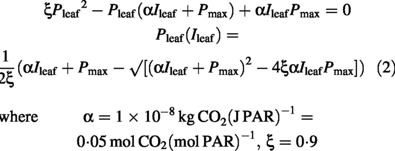
There are three parameters in this equation: α, photosynthetic efficiency, is the initial slope of the P_leaf : I_leaf curve; P_max is the light‐saturated value of photosynthesis; and ξ determines the sharpness in the knee of the curve (e.g. Thornley and Johnson, 2000, p. 228). The inverse of photosynthetic efficiency is the quantum requirement. This is approx. 19 absorbed quanta per CO₂ fixed for C₄ leaves, and varies between 15 and 22 for C₃ leaves, depending on temperature (Jones, 1992, pp. 204–205). By varying ξ from 0 to 1, eqn (2) varies from a rectangular hyperbola (RH) to two intersecting straight lines [a ‘limiting factor’ or Blackman‐like response (Blackman, 1905)]. The much improved fit generally obtained with the three‐parameter NRH as compared with the two‐parameter RH is wide ly accepted (e.g. Boote and Loomis, 1991; Jones, 1992, p. 203). However, estimating ξ from data is difficult, especially for high‐light grown leaves, and estimates are very variable (Leverenz, 1987; Ogren and Evans, 1993). The value of ξ is usually determined by curve‐fitting; values in the range 0·5–0·95 are commonly observed (Lieth and Reynolds, 1987). Our ‘typical’ value of 0·9 is at the upper end of the range, a value which gives clear differentiation from a RH with ξ = 0. For the latter case (a RH with ξ = 0), a simpler analysis as carried out by Medlyn et al. (2000, equation A7) leads to eqn (18). When non‐linear effects caused by sun and shade are considered, an accurate representation of the central part of the response is required. As with eqn (1) for light interception, eqn (2) for leaf photosynthesis provides a realistic phenomenology which has been widely used (e.g. Marshall and Biscoe, 1980; Terashima and Saeki, 1985; Leverenz, 1995), and is derivable from a simple scheme (e.g. Thornley and Johnson, 2000, pp. 226–228). It is usual to assume that α and ξ are constant down the canopy (with increasing L), although this simplifying assumption is not realistic for P_max, and may be deficient for ξ.

Photosynthetic acclimation

P_max can acclimate to conditions and assumes a wide range of values (Prioul et al., 1980; Evans and Terashima, 1988; Pettersson and McDonald, 1994; Hikosaka and Terashima, 1996; Walcroft et al., 1997; Kull and Niinemets, 1998). This acclimation typically takes about 1 week, a time substantially longer than diurnal variations in light. The factors affecting acclimation are, roughly in order of importance, light level, nitrogen nutrition, ambient carbon dioxide (CO₂) concentration and temperature. Many of the studies cited above address the question of N distribution in the canopy, and whether or not this is optimal for canopy photosynthesis. Some report that N is optimally distributed and some conclude that the distribution is not optimal. Such conclusions are always the result of running a model with its attendant uncertainties, and not of direct measurement. There is no consensus, but Hollinger (1996) concludes by saying ‘in the meantime, modellers may wish to follow the pragmatic approach and allocate N as a linear function of the microsite PPFD’ (PPFD = photosynthetic photon flux density). Essentially this is what we do, following Charles‐Edwards (1981, p. 70), who suggested that an adequate approximation to acclimation of P_max down the canopy is:

P_max0 is the value of P_max for fully exposed leaves at the top of the canopy. The value given is a rounded but not atypical value. For C₃ and C₄ leaves, respectively, Jones (1992, table 7·3, p. 190) gives ranges of 11 to 27, and 14 to 55 µmol m^–2 s^–1. While eqn (3) probably overstates the decrease in P_max, especially towards the bottom of a high LAI canopy, this is relatively unimportant as in high LAI canopies most of the canopy photosynthesis is from the upper third of the canopy (Acock et al., 1978); it is important to have an appropriate value for P_max0, the value at the top of the canopy. P_max0 may be determined empirically, or alternatively, by means of an acclimation sub‐model (e.g. Thornley, 1998b). An assumption equivalent to eqn (3) has often been made in calculations of canopy photosynthesis (e.g. Sands, 1995; De Pury and Farquhar, 1997).

Sun and shade leaves

To complete the basic equations required, the components of leaf area index, L, and an increment in L, dL, exposed to sun and shade, are:

The irradiance of a horizontal surface above the canopy, I₀ (J PAR m^–2 s^–1), comprises two components, diffuse light (dif) and direct sun (sun), with:

The fraction f_sun, varying between 0 and 1, allows relative amounts of diffuse and direct light to be easily varied. f_sun varies diurnally and seasonally (Jones, 1992, p. 23, reports data from Anon, 1980), and this variation must be simulated when this analysis is applied within a larger model. Irradiances of sunlit and shaded leaves at depth L in the canopy are assumed to be [cf. eqn (1)]:

This assumes leaves of random orientation; the contribution of scattered sunlight to diffuse light is ignored.

ANALYSIS

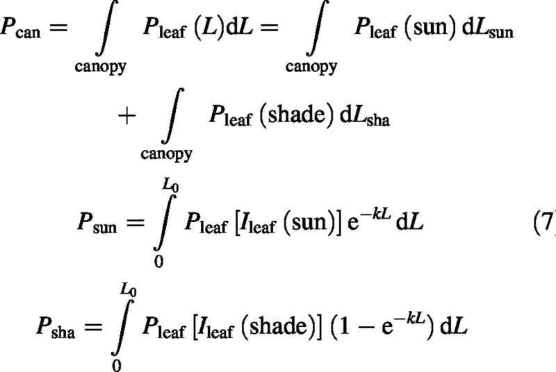
Canopy photosynthesis, P_can (kg CO₂ m^–2 s^–1) and its sun and shade components, P_sun and P_sha, are given by the integrals [with eqn (4)]:

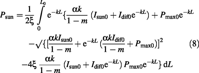
Sun–leaf canopy photosynthesis is [eqns (6), (2) and (3)]:

Substitute

Therefore

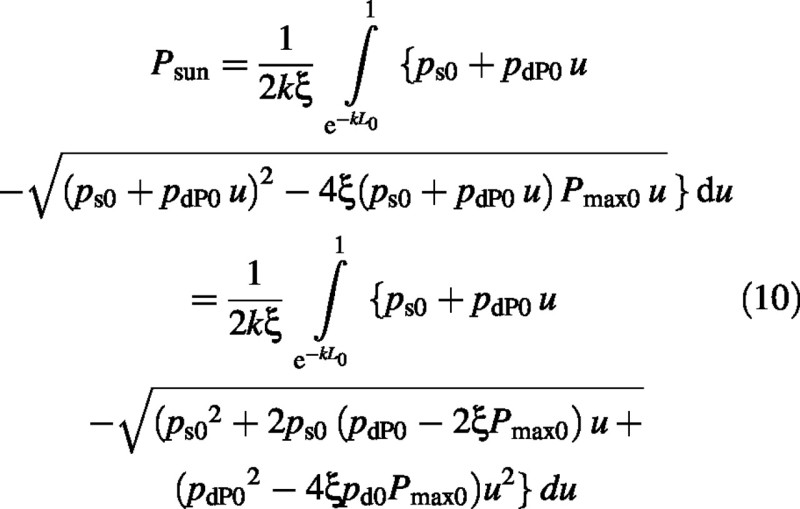
A second substitution is made of

Hence

The integral is a standard form (Gradshteyn and Ryzhik, 1994) (c > 0 which is always true here):

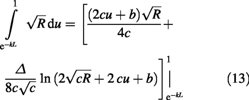
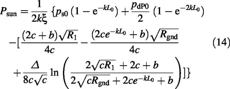
Finally the sun–leaf component of the canopy photosynthetic rate is:

The shade–leaf canopy photosynthesis component is more easily derived [eqns (7), (6), (2) and (3)]:

Substitute from eqn (9) to give:

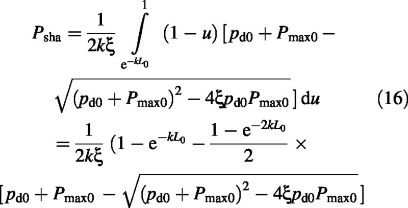
Note that the effects of LAI (L₀) and light [I₀ (p_d0), eqn (9)] factorize.

It can be useful to calculate sun and shade contributions separately because, for reasons such as differential stomatal closure, it may be necessary to modify them differently before summing to obtain canopy photosynthesis.

With f_sun = 0 and no direct solar radiation, both sun and shade leaves contribute to canopy photosynthesis, although now the sun leaves only receive diffuse irradiance. In this case it can be shown that [apply 0 = f_sun = I_sun0= p_s0= a = b = Δ in eqn (14); see eqns (5), (9) and (11)]:

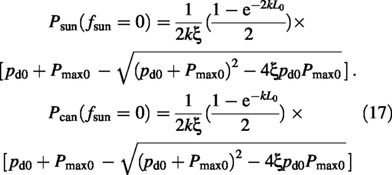
Again note that the effects of LAI (L₀) and irradiance [I₀ (p_d0), eqn (9)] factor out, lending credibility to a possible simple modelling approach which treats LAI‐ and irradiance‐dependence as independent factors. Furthermore, if P_max0 ∼ I₀ [eqns (3) and (5); whether this is valid will depend on the mechanism of acclimation and the conditions], then the term in [...] is linear in I₀, photosynthesis is proportional to intercepted light, giving credence to linear models of crop productivity (Monteith, 1977).

For the simpler rectangular hyperbola [ξ = 0 in eqn (2)], the sun and shade contributions are:

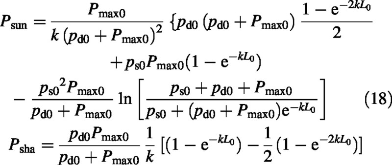
These equations agree with Medlyn et al. (2000, equation A7) who give total photosynthesis only.

RESULTS AND DISCUSSION

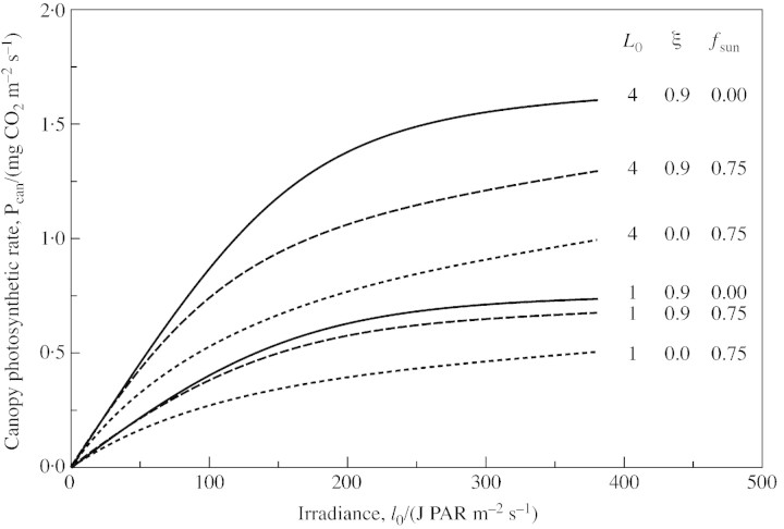
Total canopy photosynthesis [eqn (7)] is drawn in Fig. 1 for two leaf area indices (LAI, L₀) with three cases: (1) radiation all diffuse [f_sun = 0; eqn (5)] and using the non‐rectangular hyperbola (NRH) with ξ = 0·9 giving a sharp knee to the leaf response [eqn (2)]; (2) 75 % direct solar radiation (f_sun = 0·75) with the same NRH for leaf response (ξ = 0·9); and (3) 75 % direct solar radiation with ξ = 0 giving a rectangular hyperbola for leaf response that is far more curved than the NRH although with the same initial slope and asymptote. The differences between (1) and (2) are small at low LAI where most leaves are similarly illuminated, becoming more important at high LAI because there are now more shaded leaves. Indeed, at low light, all three curves for a given LAI have the same initial slope; photosynthetic rate is independent of ξ and the direct‐sun fraction, f_sun; all leaves are on the early part of the light‐response curve with the same slope. At high light, they all approach the same asymptote when all leaves in the canopy are saturated. Use of an assumed RH (ξ = 0) can greatly underestimate canopy photosynthesis under conditions of sun and shade where the actual leaf response is more Blackman‐like with ξ closer to unity [see eqn (2) and text thereafter]. It is then important to use a leaf response function such as the NRH with an appropriate value of ξ. In sunny conditions, the difference to estimated canopy photosynthesis between treating all the radiation as diffuse and allowing as above for sun– and shade–leaf contributions can be 20 %. This difference is sufficiently large that many will not wish to ignore it. In some cases of higher LAI, assuming an RH applies where in fact an NRH gives a better description, and ignoring the sun/shade dichotomy, gives roughly a correct result—that is, a result similar to that obtained using the NRH and the sun/shade expressions.

Fig. 1. Canopy photosynthetic response to radiation at two values of leaf area index (L₀) allowing for sun– and shade–leaf contributions [eqns (14), (16) and (7)]. Parameters are as given in eqns (1)–(3), with values of f_sun [fraction of direct sunlight, eqn (5)] and ξ [parameter of the non‐rectangular hyperbola, eqn (2)] as stated. ξ = 0·9 corresponds to a non‐rectangular hyperbola with a sharp knee; ξ = 0 corresponds to a rectangular hyperbola. f_sun = 0 gives diffuse radiation only; with f_sun = 0·75, 75 % of the radiation incident on an exposed horizontal surface is direct from the sun. Alternative units: 1 mg CO₂ = 22·7 µmol CO₂; 1 J PAR = 4·6 µmol quanta of wavelength 0·55 µm.

Validation is an issue with many biologists. With a mechanistic approach, as used here, various approaches are possible. Validation at the level of the model’s predictions is a weak validation, and, as discussed by Hopkins and Leipold (1996), is often inconclusive and can be positively misleading. Moreover, validation at the predictive level may not be possible because, as probably applies here, adequate measurements cannot be made. As stated many years ago by de Wit (1970), the person who principally pioneered crop modelling, predictive‐level tuning and validation can be ‘a disastrous way of working . . . the technique reduces into the most cumbersome and subjective technique of curve‐fitting that can be imagined’. No‐one has successfully addressed the problem of what a satisfactory predictive‐level validation experiment would consist of. Some modellers find such work to be almost meaningless, and this is not to deny that a model can fail seriously at the predictive level and that these failures must be investigated and corrected. Validity is not a property of a model per se. It is a concept that pertains to the model in relation to (subjective) objectives and a sphere of application. A model may be valid for some purposes but not for others. De Pury and Farquhar (1997) ‘validate’ their sun/shade big‐leaf canopy photosynthesis model by comparison with a benchmark numerical multi‐layer model that is assumed to be acceptably correct in its predictions. Notably, they fail to address the theoretical and/or empirical status of all the procedures and assumptions they used in constructing their model. While the predictions of a model must be examined and found acceptable, the most meaningful validation of a mechanistic model is at the level of its assumptions. Ideally, this is also the level at which parameters are assigned values and there is no scope for retrospective model tuning, as is needed in many big‐leaf models of canopy photosynthesis.

The assumptions of the current approach are laid bare in eqns (1)–(3). The rest is algebra. Equation (1) for the light profile within a canopy has a limited, although useful, validity: horizontal uniformity, randomly oriented leaves so that light from different parts of the sky is equally attenuated, and exponential decay of light within the canopy. Under such conditions, eqn (1) has been shown to work quite well. Equation (2), for leaf‐level photosynthetic response to irradiance, has a wide range of successful applications. Indeed, I am not aware of any data which cannot be satisfactorily summarized using the NRH. Some may prefer other leaf photosynthesis models but, as argued by Cannell and Thornley (1998), there are some sound reasons for using the NRH in this type of exercise. Not least, using an empirical (phenomenological) model which works well avoids all arguments about validity of assumptions in perhaps more mechanistic approaches. Empirical models can usually fit the data better than mechanistic models because they are not constrained by scientific assumptions. At the sub‐model level, as in eqns (1) and (2), a reliable phenomenology may be preferable to more mechanistic approaches, but this of course depends on objectives. Some models (e.g. Farquhar et al., 1980) are formally almost identical to the NRH, although arguably not as tractable and transparent. Equation (3), for the distribution of photosynthetic capacity within the canopy, is a pragmatic approximation (see quotation above from Hollinger, 1996). It is the precise form assumed for this equation that leads to a soluble integral. The empirical data are not sufficiently precise to lend unqualified support, or otherwise, to eqn (3), but if it is modestly accurate over the upper part of the canopy, then it probably suffices for current purposes. It may be possible to underpin eqn (3) using more mechanistic models of photosynthetic acclimation (e.g. Thornley, 1998b).

In summary, eqns (14) and (16) provide an efficient means of calculating instantaneous canopy photosynthetic rate for sunlit and shaded leaves based on concise, transparent, long‐established and much investigated sub‐models of light interception and leaf photosynthesis. Although the equations are only relevant to closed uniform canopies, they are applicable to some important crop and plant ecosystem modelling problems.

ACKNOWLEDGEMENTS

I am indebted to Roddy Dewar for comments, checking the derivation and bringing the researches of Medlyn et al. (2000) to my attention. I have been much helped by the suggestions and criticisms of reviewers and editors. This investigation has been supported by the European Union through the MEGARICH project and is a contribution towards COST 619. It also contributes to work funded by the UK Department of Environment, Food and Rural Affairs under contract 1/1/64.

Received: 27 September 2001; Returned for revision: 28 November 2001; Accepted: 18 December 2001.

References

- AcockB.1991. Modeling canopy photosynthetic response to carbon dioxide, light interception, temperature, and leaf traits. In: Boote KJ, Loomis RS, eds. Modelling photosynthesis – from biochemistry to canopy CSSA Special Publication Number 19. Madison, Wisconsin: Crop Science Society of America, Inc., American Society of Agronomy, Inc., 41–55. [Google Scholar]
- AcockB, Charles‐Edwards DA, Fitter DJ, Hand DW, Ludwig J, Warren Wilson J, Withers AC.1978. The contribution of leaves from different levels within a tomato crop to canopy net photosynthesis: an experimental examination of two canopy models. Journal of Experimental Botany 29: 815–827. [Google Scholar]
- AmthorJS.1994. Scaling CO2‐photosynthesis relationships from the leaf to the canopy Photosynthesis Research 39: 321–350. [DOI] [PubMed] [Google Scholar]
- AndersonMC.1966. Stand structure and light penetration. II. A theoretical analysis. Journal of Applied Ecology 3: 41–54. [Google Scholar]
- Anon.1980. Solar radiation data for the United Kingdom 1951–1975. Met.O. 919. Bracknell, UK: Meteorological Office. [Google Scholar]
- BlackmanFF.1905. Optima and limiting factors. Annals of Botany 19: 281–295. [Google Scholar]
- BooteKJ, Loomis RS.1991. The prediction of canopy photosynthesis. In: Boote KJ, Loomis RS, eds. Modelling photosynthesis – from biochemistry to canopy CSSA Special Publication Number 19. Madison, Wisconsin: Crop Science Society of America, Inc., American Society of Agronomy, Inc., 109–140. [Google Scholar]
- CannellMGR, Thornley JHM.1998. Temperature and CO2 responses of leaf and canopy photosynthesis: a clarification using the non‐rectangular hyperbola model of photosynthesis. Annals of Botany 82: 883–892. [Google Scholar]
- Charles‐EdwardsDA.1981. The mathematics of photosynthesis and productivity. London: Academic Press. [Google Scholar]
- Charles‐EdwardsDA.1982. Physiological determinants of crop growth. Sydney: Academic Press. [Google Scholar]
- ChartierP.1966. Étude théorique de l’assimilation brute de la feuille. Annales de Physiologie Végétale 8: 167–195. [Google Scholar]
- ChertovOG, Komarov AS, Nadporozhskaya M, Bykhovets SS, Zudin SL.2001. ROMUL – a model of forest soil organic matter dynamics as a substantial tool for forest ecosystem modeling. Ecological Modelling 138: 289–308. [Google Scholar]
- CowanIR.1968. The interception and absorption of radiation in plant stands. Journal of Applied Ecology 5: 367–379. [Google Scholar]
- De PuryDGG, Farquhar GD.1997. Simple scaling of photosynthesis from leaves to canopies without the errors of big‐leaf models. Plant, Cell and Environment 20: 537–557. [Google Scholar]
- De WitCT.1970. Dynamic concepts in biology. In: Setlik I, ed. Prediction and measurement of photosynthetic productivity The Netherlands, Wageningen: Pudoc, 17–23. [Google Scholar]
- De WitCT, Brouwer R, Penning de Vries FWT.1970. The simulation of photosynthetic systems. In: Setlik I, ed. Prediction and measurement of photosynthetic productivity The Netherlands, Wageningen: Pudoc, 47–70. [Google Scholar]
- EnquistBJ, Brown JH, West GB.1998. Allometric scaling of plant energetics and population density. Nature 395: 163–165. [Google Scholar]
- EvansJR, Terashima I.1988. Photosynthetic characteristics of spinach leaves grown with different nitrogen treatments. Plant and Cell Physiology 29: 157–165. [Google Scholar]
- FarquharGD, von Caemmerer S, Berry JA.1980. A biochemical model of photosynthetic CO2 assimilation in leaves of C3 species. Planta 149: 78–90. [DOI] [PubMed] [Google Scholar]
- GradshteynIS, Ryzhik JW.1994. In: Jeffrey A, ed. Tables of integrals, series and products. Boston: Academic Press. [Google Scholar]
- HikosakaK, Terashima I.1996. Nitrogen partitioning among photosynthetic components and its consequence in sun and shade plants. Functional Ecology 10: 335–343. [Google Scholar]
- HollingerDY.1996. Optimality and nitrogen allocation in a tree canopy. Tree Physiology 16: 627–634. [DOI] [PubMed] [Google Scholar]
- HopkinsJC, Leipold RJ.1996. On the dangers of adjusting the parameter values of mechanism‐based mathematical models. Journal of Theoretical Biology 183: 417–427. [DOI] [PubMed] [Google Scholar]
- IdsoSB, de Wit CT.1970. Light relations in plant canopies. Applied Optics 9: 177–184. [DOI] [PubMed] [Google Scholar]
- JohnsonIR, Thornley JHM.1984. A model of instantaneous and daily canopy photosynthesis. Journal of Theoretical Biology 107: 531–545. [Google Scholar]
- JonesHG.1992. Plants and microclimate. Cambridge, UK: Cambridge University Press. [Google Scholar]
- KullO, Kruijt B.1998. Leaf photosynthetic light response: a mechanistic model for scaling photosynthesis to leaves and canopies. Functional Ecology 12: 767–777. [Google Scholar]
- KullO, Niinemets Ü.1998. Distribution of leaf photosynthetic properties in tree canopies: comparison of species with different shade tolerance. Functional Ecology 12: 472–479. [Google Scholar]
- LeverenzJW.1987. Chlorophyll content and the light response curve of shade adapted canifer needles. Physiologia Plantarum 71: 20–29. [Google Scholar]
- LeverenzJW.1995. Shade shoot structure of conifers and the photosynthetic response to light at two CO2 partial pressures. Functional Ecology 9: 413–421. [Google Scholar]
- LiethJH, Reynolds JF.1987. The nonrectangular hyperbola as a photosynthetic light response model: geometrical interpretation and estimation of the parameter Θ. Photosynthetica 21: 363–366. [Google Scholar]
- MarshallB, Biscoe PV.1980. A model for C3 leaves describing the dependence of net photosynthesis on irradiance. I. Derivation. Journal of Experimental Botany 31: 29–39. [Google Scholar]
- MedlynBE, McMurtrie RE, Dewar RC, Jeffreys MP.2000. Soil processes dominate the long‐term response of forest net primary productivity to increased temperature and atmospheric CO2 concentration. Canadian Journal of Forest Research 30: 873–888. [Google Scholar]
- MonsiM, Saeki T.1953. Über den Lichtfaktor in den Pflanzengesellschaften und seine Bedeutung für die Stoffproduktion. Japanese Journal of Botany 14: 22–52. [Google Scholar]
- MonteithJL.1977. Climate and the efficiency of crop production in Britain. Philosophical Transactions of the Royal Society, London B 281: 277–294. [Google Scholar]
- MonteithJL, Unsworth M.1990. Principals of environmental physics. London: Arnold. [Google Scholar]
- NormanJM, Welles JM.1988. Radiative transfer in an array of canopies. Agronomy Journal 75: 481–488. [Google Scholar]
- OgrenE, Evans JR.1993. Photosynthetic light‐response curves. I The influence of CO2 partial pressure and leaf inversion. Planta 189: 182–190. [Google Scholar]
- PetterssonR, McDonald JS.1994. Effects of nitrogen supply on the acclimation of photosynthesis to elevated CO2 Photosynthesis Research 39: 389–400. [DOI] [PubMed] [Google Scholar]
- PrioulJ‐L, Brangeon J, Reyss A.1980. Interaction between external and internal conditions in the development of photosynthetic features in a grass leaf. I. Regional responses along a leaf during and after low‐light or high‐light acclimation. Plant Physiology 86: 762–769. [DOI] [PMC free article] [PubMed] [Google Scholar]
- RabinowitchEI.1951. Photosynthesis and related processes, 2(1). New York: Interscience. [Google Scholar]
- SandsPJ.1995. Modelling canopy production. II. From single leaf photosynthetic parameters to daily canopy photosynthesis. Australian Journal of Plant Physiology 22: 593–601. [Google Scholar]
- SheehyJE, Cobby JM, Ryle GJA.1980. The use of a model to investigate the influence of some environmental factors on the growth of perennial ryegrass. Annals of Botany 46: 343–365. [Google Scholar]
- SinclairTR, Horie T.1989. Leaf nitrogen, photosynthesis, and crop radiation use efficiency: a review. Crop Science 29: 90–98. [Google Scholar]
- SzeiczG.1974. Solar radiation in plant canopies. Journal of Applied Ecology 11: 1117–1156. [Google Scholar]
- TerashimaI, Saeki T.1985. A new model for leaf photosynthesis incorporating the gradients of light environment and of photosynthetic properties of chloroplasts within a leaf. Annals of Botany 56: 489–499. [Google Scholar]
- ThornleyJHM.1998a Grassland dynamics: an ecoystem simulation model. Wallingford, Oxon: CAB International. [Google Scholar]
- ThornleyJHM.1998b Dynamic model of leaf photosynthesis with acclimation to light and nitrogen. Annals of Botany 81: 421–430. [Google Scholar]
- ThornleyJHM, Johnson IR.2000. Plant and crop modelling. A mathematical approach to plant and crop physiology Reprint of 1990 Oxford University Press edition. www.blackburnpress.com [Google Scholar]
- WalcroftAS, Whitehead D, Silvester WB, Kelliher FM.1997. The response of photosynthetic model parameters to temperature and nitrogen concentration in Pinus radiata D. Don. Plant, Cell and Environment 20: 1338–1348. [Google Scholar]
- WangYP, Jarvis PG.1990. Description and validation of an array model – MAESTRO. Agricultural and Forest Meteorology 51: 257–280. [Google Scholar]
- WhitfieldDM.1980. Simulated response of tobacco crops to irradiance and defoliation. Australian Journal of Plant Physiology 7: 487–500. [Google Scholar]
- WohlfahrtG, Bahn M, Cernusca A.1999. The use of the ratio between the photosynthesis parameters Pml and Vcmax for scaling up photosynthesis of C3 plants from leaves to canopies: a critical examination of different modelling approaches. Journal of Theoretical Biology 200: 163–181. [DOI] [PubMed] [Google Scholar]
Associated Data
This section collects any data citations, data availability statements, or supplementary materials included in this article.