The Neural Circuit Mechanisms Underlying the Retinal Response to Motion Reversal

Abstract

To make up for delays in visual processing, retinal circuitry effectively predicts that a moving object will continue moving in a straight line, allowing retinal ganglion cells to anticipate the object's position. However, a sudden reversal of motion triggers a synchronous burst of firing from a large group of ganglion cells, possibly signaling a violation of the retina's motion prediction. To investigate the neural circuitry underlying this response, we used a combination of multielectrode array and whole-cell patch recordings to measure the responses of individual retinal ganglion cells in the tiger salamander to reversing stimuli. We found that different populations of ganglion cells were responsible for responding to the reversal of different kinds of objects, such as bright versus dark objects. Using pharmacology and designed stimuli, we concluded that ON and OFF bipolar cells both contributed to the reversal response, but that amacrine cells had, at best, a minor role. This allowed us to formulate an adaptive cascade model (ACM), similar to the one previously used to describe ganglion cell responses to motion onset. By incorporating the ON pathway into the ACM, we were able to reproduce the time-varying firing rate of fast OFF ganglion cells for all experimentally tested stimuli. Analysis of the ACM demonstrates that bipolar cell gain control is primarily responsible for generating the synchronized retinal response, as individual bipolar cells require a constant time delay before recovering from gain control.

Introduction

Time delays are an inescapable consequence of signal transmission in any biological or physical system. In the retina, delays inherent to the process of visual transduction by the photoreceptors (Schnapf et al., 1987) prevent ganglion cells from transmitting responses to the primary visual cortex until 30–100 ms after light reaches the retina (Lennie and Perry, 1981). To compensate for this delay, ganglion cells anticipate object motion by effectively predicting that a moving object will continue to move in a straight line (Berry et al., 1999).

But what happens when an object suddenly changes direction and the retina's prediction turns out to be wrong? While a cheetah can outrun an antelope over short distances, the antelope eludes capture by zigzagging and changing direction. Being able to rapidly detect these missed predictions and reset the retina's anticipatory mechanisms would obviously be of great survival benefit for the cheetah. In the case of reversals of direction, previous work has shown that the retina can signal a reversal via synchronized firing among a large population of ganglion cells (Schwartz et al., 2007). This response occurs in approximately one-third of salamander ganglion cells and always occurs at a fixed latency after reversal regardless of reversal position. Retinal ganglion cells can respond to reversals of objects at different speeds, sizes, and contrasts.

To further elucidate the neural circuit mechanisms underlying the reversal response, we used a combination of multielectrode array (MEA) recordings and whole-cell patch recordings of retinal ganglion cells in the tiger salamander (Ambystoma tigrinum). We investigated the single-cell responses to reversing bars and edges of different polarity and found that ganglion cells were responsive to the reversal of some but not all tested objects (e.g., reversal responsive to dark bars but not dark edges, or vice versa). Pharmacological manipulations with the mGluR6 blocker, L-AP4, showed that the ON pathway is involved in generating the reversal response to a dark edge and, in certain cases, a dark bar. Whole-cell patch recordings revealed that the responses to motion reversal were caused primarily by excitatory currents. In support of this conclusion, blockage of inhibitory neurotransmission did not abolish the reversal response.

To understand these visual computations, we applied the adaptive cascade model (ACM), which was developed to describe the synchronized firing of ganglion cells to the sudden onset of motion (Chen et al., 2013); this model incorporated gain control and rectification at both the bipolar and ganglion cell stages. The ACM could accurately reproduce the reversal response, as well as the responses to several other motion discontinuities (sudden start, stop, and two-fold acceleration) and the cases of two bars crossing or moving in tandem. Analysis of the ACM revealed that, although all the stages of the model contributed in detail to the reversal response, bipolar cell gain control played the key role in generating a reversal response synchronized across ganglion cells.

Materials and Methods

MEA recordings.

MEA recordings were performed according to the methods detailed by Chen et al. (2013). Stimuli were displayed on a computer monitor (Puchalla et al., 2005) at a frame rate of 60 Hz and focused onto the photoreceptor layer with standard optics. Motion reversal stimuli consisted of a bar of light (width = 162 μm) or an edge moving at 1.62 mm/s, unless otherwise noted. Bars/edges reversed at 6 or 10 positions centered on the MEA that were spaced 81 μm apart. Receptive fields were calculated using reverse correlation to random flicker (sixty 54 μm strips oriented parallel to the moving bar stimuli) displayed at 30 Hz.

Patch-clamp recordings.

All recordings were made according to the methods detailed previously (Soo et al., 2011). In brief, retinas from tiger salamanders of either sex (Ambystoma tigrinum) were dissected and placed in the whole-mount preparation and viewed under infrared illumination. Individual ganglion cells were patched using standard whole-cell patch techniques. Patch electrodes were pulled from borosilicate glass, had tip diameters of 1.0–1.5 μm, and had resistances of 6–12 mΩ. Recordings were filtered at 400 Hz, sampled at 10 kHz, and recorded with custom software written in Labview (National Instruments).

Visual stimulation was delivered using an RGB LED (SuperbrightLEDS) focused through a holographic diffuser (ThorLabs) onto a digital mirror device (Discovery 3000, Texas Instruments) projected through a 10× apochromatic objective (Nikon) mounted in place of the condenser of the microscope (Nikon FN-1). Light levels were calibrated to match the photoreceptor spectra previously reported (Makino et al., 1991; Ma et al., 2001). Motion reversal stimuli consist of bars (width 168 μm) and edges moving at a speed of 1.72 mm/s. Bars/edges reversed at 10 different positions 57.6 μm apart. Stimuli were projected a frame rate of 1440 Hz.

Measuring the reversal response.

All peristimulus time histograms were constructed using 25 ms time bins and averaging over all repeated presentation of the same stimulus. Following Schwartz et al. (2007), individual ganglion cells were judged to be “reversal responsive” if they had a peak in their firing rate >10 Hz in a time window between 150 and 300 ms after the time of an object's motion reversal; in addition, such a peak had to be present in at least three different reversal locations. This classification was performed independently for each kind of moving object (for instance, a cell could be reversal responsive to the dark bar but not the dark edge).

For most of our analysis, a population average firing rate was constructed by averaging over the individual peristimulus time histograms of all the ganglion cells that were reversal responsive to a particular kind of moving object. In many cases, we wanted to resolve this response as a function of the location of motion reversal on ganglion cells' receptive fields. To this end, we averaged the individual peristimulus time histograms of reversal responsive ganglion cells for all of the conditions in which the location of the reversal was within a narrow spatial range, typically ±41 μm, on that cell's receptive field.

Receptive fields.

Receptive fields were calculated in the same manner as described by Chen et al. (2013). By determining the spatial receptive fields from our experimentally recorded data, we were able to set our receptive field properties independent from the ACM and thus reduce the number of free parameters in our model. Briefly, the (time-reversed) spike-triggered average response to random flicker stimulation was defined as K(x, t). To calculate the spatial kernel of the ganglion cell receptive field, K(x*, t) was first estimated, where x* represents the spatial location of the extremal response. The projection of each temporal response at each point in space onto the extremal response was then fit to a difference of Gaussians to determine the spatial kernel, B_G(x), as follows:

Where x₀ is the center coordinate, B_c and B_s are the relative strengths of the center and surround, and Σ_c and Σ_s represent their respective radii. The temporal kernel, C_G(t), was calculated by computing the average temporal response over the receptive field center as follows:

Spatial kernels were then normalized such that their peak values were equal to 1, and temporal kernels were normalized such that their vector norm was 1.

ACM with ON and OFF bipolar cells.

The model used for motion reversal was based on the adaptive cascade model (ACM) described by Chen et al. (2013). We first outline the original structure of the ACM and then describe the modifications made to ACM in this present work. The ACM features an array of bipolar cell subunits in the ganglion cell's receptive field; each subunit was taken to be an individual bipolar cell. Because all stimuli moved in only one spatial dimension, we used a 1D array with bipolar cells spaced 5 μm apart and centered at x_i. Each bipolar cell spatiotemporal kernel, k_i(x, t), was proportionally similar to the experimentally calculated ganglion cell spatial (B_G) and temporal kernels (C_G) but scaled down to a center radius of σ_c = 25 μm (a value based on published data for salamander bipolar cells) (Baccus et al., 2008). Thus, convolution of each bipolar cell kernel with the stimulus, s(x, t), yielded the bipolar soma voltage, V_i(t), as follows:

The bipolar soma voltage was then passed through a nonlinear function, N_i(t), and a gain control function, G_i(t), with a time-dependent activation, A_i(t), to convert the soma voltage to glutamate release, R_i(t). These functions were defined as follows:

Next, the bipolar synaptic outputs were combined by the ganglion cell through a synaptic weighting function: w_i = B_G(x_i), where B_G(x_i) is a difference of Gaussian function derived from the ganglion cell's experimentally recorded spatial kernel. Thus, the ganglion cell soma voltage was as follows:

Finally, to determine the firing rate of the ganglion cell, another set of nonlinear (N_G(t)) and gain control (G_G(t)) functions at the ganglion cell level transformed the ganglion cell soma voltage to a firing rate, R_G(t).

The original form of the ACM was able to capture the ganglion responses to smooth motion and motion onset, but for it to reproduce the response to motion reversal, we found that it was necessary to incorporate ON bipolar cells into the model. The bipolar cell stages of the ACM were therefore duplicated into parallel ON and OFF pathways. For example, the soma voltage of the ACM, which was previously V_i(t) in Chen et al. (2013), was now duplicated into V_ONi(t) and V_OFFi(t), which subsequently led to corresponding nonlinear (N_ONi(t) and N_OFFi(t)) and bipolar output (R_ONi(t) and R_OFFi(t)) functions. The only difference between the two pathways was that the ON bipolar cell temporal kernel, C_ON, was defined as a scaled-down version of the ganglion cell temporal kernel with opposite polarity:

This matches reasonably well the ON polarity filters found for ganglion cells through spike-triggered covariance methods (Fairhall et al., 2006; Geffen et al., 2007; Gollisch and Meister, 2008). Although there are some asymmetries between the ON and OFF pathways (Chander and Chichilnisky, 2001; Rieke, 2001; Beaudoin et al., 2008), our goal was to construct a minimal model to explain our data. As such, we avoided adding additional free parameters to the model if they were not clearly required.

Fast OFF ganglion cells receive stronger input from the OFF pathway compared to the ON pathway, as evidenced by their OFF-polarity spike-triggered averages. Other models have accounted for this different weighting by having a lower threshold nonlinear function (Geffen et al., 2007) or by normalizing the two filters such that their sum equaled the ganglion cell filter (Gollisch and Meister, 2008). We chose to implement this weighting by scaling the response of each pathway by a factor, ϕ, such that the ganglion cell soma voltage was now defined as follows:

The relative weights of the ON and OFF pathway vary considerably from cell to cell (Fairhall et al., 2006; Geffen et al., 2007; Garvert and Gollisch, 2013). To best match the firing rate averaged over the entire population of fast OFF cells, we used a ϕ value of 0.15. The other model parameters that were used for motion reversal are listed in Table 1. In particular, we note that the parameter values for the ON and OFF pathways were taken to be identical, in accordance with the goal of constructing a minimally complex model. Parameters were fit using an automated minimization function (“fmincon,” MATLAB 2013; MathWorks).

Table 1.

Parameters of the adaptive cascade model^a

Parameter	Description	Retina 1	Retina 2
θB	Bipolar cell threshold	6.52	5.215
HB	Amplitude of bipolar cell gain control	0.981	0.975
τB	Time constant of bipolar cell gain control	134 ms	125 ms
θG	Ganglion cell lower threshold	0	0
NGmax	Ganglion cell upper threshold	450	450
αG	Scale of ganglion cell output	2.88	2.33
HG	Amplitude of ganglion cell gain control	0.0369	0.0342
τG	Time constant of ganglion cell gain control	48 ms	38 ms

^aValues of the free parameters of the ACM that were optimized for best fit with experimental data.

Finally, we note that a key technical detail in the successful implementation of the ACM was the fact that we fixed all of the parameters that characterized the classical receptive field. These parameters included the temporal kernel as well as the synaptic weights that determined the ganglion cell's spatial profile. Our method was to focus on ganglion cells of a single functional type; because these cells had exceptionally similar temporal profiles, we could simply use their average measured temporal profile as the kernel in the ACM. Furthermore, all experimental data consisted of averages over the measured firing rates of many ganglion cells. Although individual ganglion cells possessed strong “hot spots” in their spatial receptive fields (Soo et al., 2011), these hot spots were smoothed by averaging over a large population. As a result, the ACM could use a generic spatial profile with a width matched to data. Because all of these receptive field parameters were fixed by experimental measurement, we were left with only eight free parameters that we needed to optimize to explain our reversal response data. If we instead needed to optimize the values of scores more parameters for the temporal dynamics and spatial hot spots of the receptive field, we might not have been able to find successful and reproducible model parameters.

Results

Ganglion cells of different functional types can be reversal responsive

In response to motion reversal, salamander retinal ganglion cells fire a transient burst of firing ∼250 ms after reversal. Following a previous study, we defined cells as “reversal responsive” if the latency of this response was constant for reversal positions over a range of at least 110 μm (Schwartz et al., 2007). This previous study found that approximately one-third (37%) of ganglion cells were reversal responsive and that reversal responses were present in the ganglion cell population for both ON and OFF moving bars. However, individual ganglion cells were not analyzed under different stimulus conditions. To this end, we used a 252-electrode MEA to record ganglion cell responses to different motion reversal stimuli. As in Schwartz et al. (2007), we determined the average reversal response of a population of ganglion cells by averaging over all positions where a cell was reversal responsive (Fig. 1, blue line). To calculate the corresponding smooth motion response of this population, we matched the smooth motion response to each individual reversal such that before reversal both stimuli were identical. We then averaged over all these matched smooth motion responses to determine the population average (Fig. 1, red line).

Figure 1.

Reversal responses to different types of reversing objects. Average responses of 31 reversal responsive cells to bright/dark bars and edges moving in smooth motion (red) as well as reversing direction (blue). Responses were averaged over all positions where a cell was reversal responsive. Smooth motion responses were aligned such that, before motion reversal, the both smooth and reversal stimuli were identical. A, Reversal of an OFF bar. B, Reversal of an ON bar. C, Reversal of an OFF edge. D, Reversal of an ON edge.

Having confirmed that we could identify populations of reversal responsive ganglion cells, we then classified individual reversal responsive cells according to the functional cell types described by Segev et al. (2006). We found that there was not a single cell type that was reversal responsive. Instead, reversal responses were primarily present in three cell types: fast OFF (110 of 375 cells = 29% were reversal responsive in at least one stimulus condition), medium OFF (19 of 112 = 17%), and fast ON (21 of 51 = 41%). Very few of either slow OFF or medium ON cells were found to be reversal responsive (<10 of 600). Similar results were found for ganglion cells in the mouse: fast OFF had reversal responses in 5 of 11 = 45% of cells, medium OFF had 8 of 33 = 24%, and fast ON had 6 of 20 = 30%.

Of note, we did not find a categorical distinction between a reversal responsive cell and a non-reversal responsive cell. Instead, ganglion cells appeared to exhibit a broad variety of reversal peak strengths. For this study, we used relatively conservative criteria for defining a cell as reversal responsive. Of the two criteria used to assess reversal responsiveness (robust response and fixed response latency) a significant proportion of cells met at least one of the criterion but not both (e.g., for fast OFF cells in salamander, 164 of 375 cells had at least a 10 Hz peak in the firing rate following motion reversal and 263 of 375 had a peak at constant latency, but only 110 cells met both criteria).

Reversal responsive cells are responsive to specific reversals

Although the previous study found reversal responsive cells for both bright and dark bars as well as for dark edges, it was still unknown whether reversal responsive cells responded to every kind of reversing object or whether specific subsets of cells respond to the reversal of specific objects. We sought to answer this question by comparing the responses of individual ganglion cells with these different kinds of reversing objects. If motion reversals were caused by a single circuit mechanism, then cells should be reversal responsive to multiple kinds of reversing objects. If entirely different mechanisms were responsible, then the fraction of cells responsive to one kind of reversing object should be independent of the fraction responsive to another kind of reversing object.

When we compared reversal responses of individual ganglion cells with two kinds of reversing objects, we found that relatively few cells were reversal responsive to both stimuli (Tables 2 and 3). (As a matter of terminology, if a cell is reversal responsive to only one kind of reversing object, we refer to it as being “reversal specific” to that object). Furthermore, the frequency of these cells that were reversal responsive to two different objects corresponded to the number of cells predicted if the frequency of reversal specificity was statistically independent (Tables 2 and 3, column 6). The fact that being reversal specific to a particular object does not affect the chances of a cell being reversal responsive to another condition suggests that different neural circuits, or variations of the same basic circuit, are responsible for generating responses specific to different kinds of reversing objects.

Table 2.

Classification of reversal responsive cells by stimulus type^a

	Reversal responsive	Dark bar	Dark edge	Both	Independent
Fast OFF	110	36 (33%)	24 (22%)	7	7.9
Medium OFF	19	4 (21%)	4 (21%)	1	0.8
Slow OFF	6	0	0	0	0
Fast ON	21	9 (43%)	16 (76%)	7	6.9

	Reversal responsive	Bright bar	Bright edge	Both	Independent
Fast OFF	110	69 (63%)	58 (53%)	41	36.4
Medium OFF	19	9 (47%)	7 (37%)	3	3.3
Slow OFF	6	2 (33%)	2 (33%)	1	0.7
Fast ON	21	8 (38%)	3 (14%)	1	1.1

^aFraction of ganglion cells showing a reversal response from four different retinas categorized based on which type of stimulus elicited a reversal response. Comparison of reversal responses for moving bars versus moving edges.

*.

Table 3.

Classification of reversal responsive cells by stimulus polarity^a

	Reversal responsive	Dark bar	Bright bar	Both	Independent
Fast OFF	110	36 (33%)	69 (63%)	15	22.6
Medium OFF	19	4 (21%)	9 (47%)	1	1.9
Slow OFF	6	0	2 (33%)	0	0
Fast ON	21	9 (43%)	8 (38%)	4	3.4

	Reversal responsive	Dark edge	Bright edge	Both	Independent
Fast OFF	110	24 (22%)	58 (53%)	9	12.7
Medium OFF	19	4 (21%)	7 (37%)	0	1.5
Slow OFF	6	4 (67%)	2 (33%)	1	1.3
Fast ON	21	16 (76%)	3 (14%)	2	2.3

^aFraction of ganglion cells showing a reversal response from four different retinas categorized based on which type of stimulus elicited a reversal response. Comparison of reversal responses for bright ojbects versus dark objects.

We also found that cells were generally more likely to be reversal responsive to stimuli of the opposite polarity (OFF cells were generally more likely to be reversal responsive to reversing bright objects, whereas ON cells were more likely to be reversal responsive to reversing dark objects). Of the 135 reversal responsive OFF cells, twice as many responded to reversing bright objects than dark objects (147 cells and conditions vs 72; Tables 2 and 3). The same was true for ON cells (26 cells and conditions responding to dark objects vs 11 to bright objects).

We can begin to understand these results by noting that for reversing edges, the effective polarity of the moving edge switches. For instance, a bright edge increases the light intensity on the retina as it moves, making it an event that should primarily activate the ON pathway, but after reversal, the light intensity on the retina within this dark region switches back to gray, instead activating the OFF pathway (Fig. 2B,C, left pictograms). Therefore, once a bright edge reverses, it becomes an OFF-type stimulus that can more strongly activate OFF-type ganglion cells, consistent with the finding that OFF cells were more likely to have a reversal response to a bright edge. Similarly, a dark edge is expected to generate reversal responses in a larger fraction of ON cells. The same concept applies to reversing bars, although as detailed in the following section, bars are more complex as they have both a leading and trailing edge (Fig. 2B,C, right pictograms).

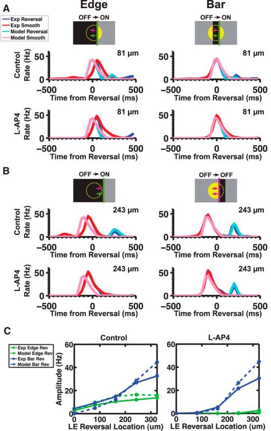
Figure 2.

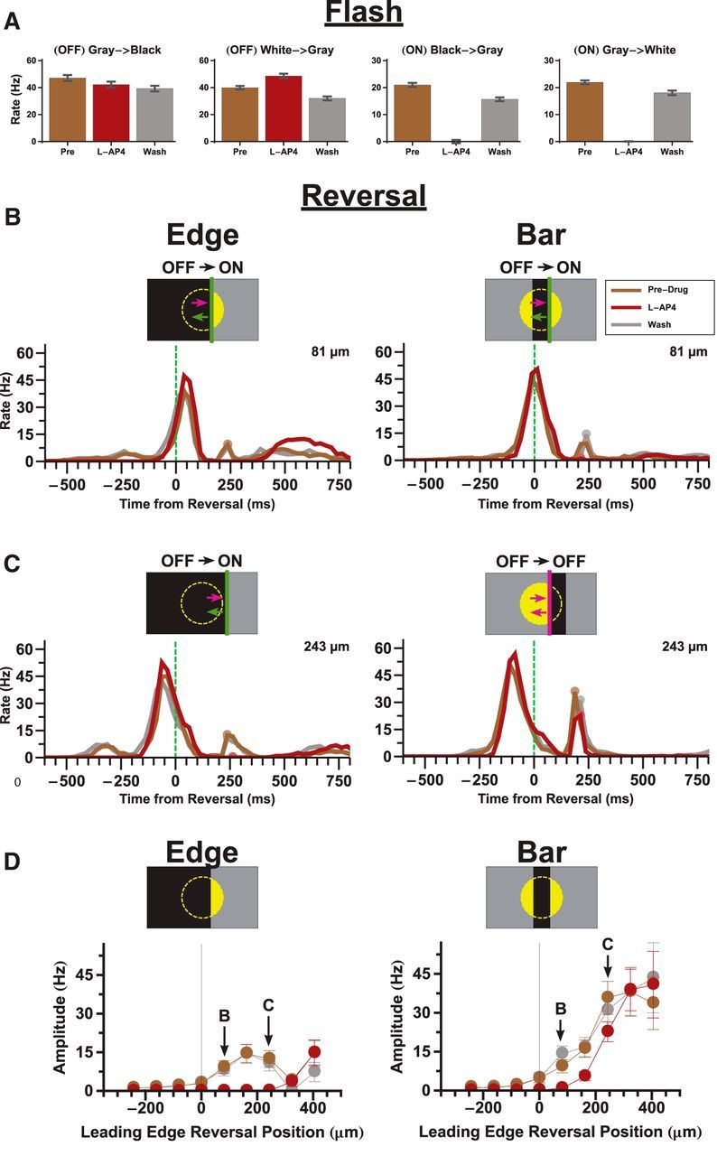
Different mechanisms of a reversal response. A, Effect of L-AP4 on the responses of 43 reversal responsive fast OFF cells to different full field flashes. B, C, Effect of L-AP4 on the responses to reversing bars (right) and edges (left) at two different distances past the cell's RF center, 81 μm (B) and 243 μm (C). The last broad lump of firing during the edges stimuli is due to the edge stimulating the RF surround. D, Effect of L-AP4 on the amplitude of the reversal responses to bars (right) and edges (left) given different reversal positions. Error bars indicate SE. Pictograms: OFF stimuli (purple), ON stimuli (green).

Because of the great heterogeneity of reversal responses among ganglion cell types and for different kinds of reversing objects, we chose to focus on just one cell type: the fast OFF cell. This cell type is quite numerous (approximately one-third of all recorded cells in the salamander) (see Segev et al., 2006, where this type was split into biphasic and monophasic OFF cells). Furthermore, this cell type is brisk and has the shortest response latency, making it likely to be particularly important for tracking moving objects (Leonardo and Meister, 2013). As an additional simplification, we chose to focus on reversal of dark objects, as there currently are no models that have been shown to capture an OFF cell's response to a bright object moving in smooth motion, a natural prerequisite to an attempt to model motion reversal.

Finally, we note that in Figure 2 and in the rest of the data that follow, we present population firing rates averaged over fast OFF ganglion cells with the added condition that the moving bar reversed within a narrow range of locations on each cell's receptive field. These more stringent criteria result in a peak firing rate after motion reversal that was systematically smaller than when we averaged over all cell types and all locations, as in Figure 1 and in the previous study (Schwartz et al., 2007). When we use the previous method of analysis, the amplitude of the reversal response was found to be consistent with the previous study.

The ON pathway is required for detecting reversals of dark edges

To further elucidate the role of the ON and OFF pathways in the generation of the reversal response, we used the mGluR6 receptor blocker, L-AP4, which abolishes light responses in ON bipolar cells (Slaughter and Miller, 1981; Yang, 2004). As expected, L-AP4 was able to completely abolish the responses to spatially uniform ON flashes (Fig. 2A). The response of a white-to-gray flash was slightly increased by L-AP4, which suggests the presence of crossover inhibition (Pang et al., 2007) from the ON pathway onto the OFF pathway (Fig. 2A, second panel). However, this crossover inhibition did not seem to be necessary for the reversal response, as blocking inhibition did not affect the reversal response (see Fig. 4).

Figure 4.

Inhibitory signaling does not abolish the reversal response. A, Effect of blocking inhibition with bicuculline (20 μm), picrotoxin (150 μm), and strychnine (5 μm) on the responses to reversing edges (left) and bars (right). The average rate is shown for the overall firing rate during the entire phase of each condition (Pre-Drug, Inhibitory Block, Washout). The bar/edge reversed at a reversal location 162 μm past the cell's RF center. B, Effect of blocking inhibition on the amplitude of the reversal responses to edges (left) and bars (right) given different reversal positions.

For a reversing dark edge, the addition of L-AP4 completely knocked out the reversal response (Fig. 2B, left, C, left). This is consistent with the interpretation that the reversal response of a dark edge is triggered by the increase in light intensity following reversal that activates the ON pathway (Fig. 2B, left pictogram). For a reversing dark bar, the situation was more complicated, as L-AP4 only affected the reversal response for some reversal locations (Fig. 2B, right). The reversal response can be triggered by either the leading or trailing edge (Schwartz et al., 2007); and when a dark bar reverses, the leading edge switches from activating the OFF pathway (which we will call an “OFF-polarity stimulus”) to activating the ON pathway (“ON-polarity stimulus”). Thus, for positions where the leading edge reverses just past the receptive field's center coordinate, blockade of the ON pathway with L-AP4 prevented the cell from responding to the reversed leading edge because this was an ON-polarity stimulus (Fig. 2B, right pictogram). But for reversal positions farther past the cell's center coordinate, the trailing edge became the main driver of the reversal response. Because this edge was an OFF-polarity stimulus after motion reversal, it was unaffected by L-AP4 (Fig. 2C, right).

The results from the L-AP4 experiments suggest that there are two different mechanisms for generating a reversal response: one dependent on the ON pathway (which operates for reversals of a dark edge and the leading edge of a dark bar) and another independent of the ON pathway (which operates for reversals of the trailing edge of a dark bar). This ON-independent mechanism presumably involves the OFF pathway.

Activation of the OFF pathway alone can generate a reversal response

To further test the ON-independent pathway, we designed two kinds of moving objects, where only the trailing edge reversed direction. For the “half-exploding bar” stimulus, the trailing edge reversed while the leading edge remained stationary after reversal. For the “full-exploding bar” stimulus, the trailing edge reversed while the leading edge instead continued moving at constant velocity (Fig. 3A). These stimuli allowed us to isolate retinal responses from the OFF pathway by eliminating substantial activation of the ON pathway following motion reversal. We found that ganglion cells that responded to the reversal of a dark bar generated a nearly identical response to both exploding bar stimuli (Fig. 3B). The “full-exploding bar” stimulus generated an additional peak in the firing rate at a time characteristic of the reversal response (150–350 ms after reversal), but this was an artifact of the leading edge continuing to move in smooth motion rather than an actual reversal response (Fig. 3C, open circles). These data strongly imply that the ON pathway is not necessary for generating a reversal response and that both the leading and trailing edges can produce reversal responses.

Figure 3.

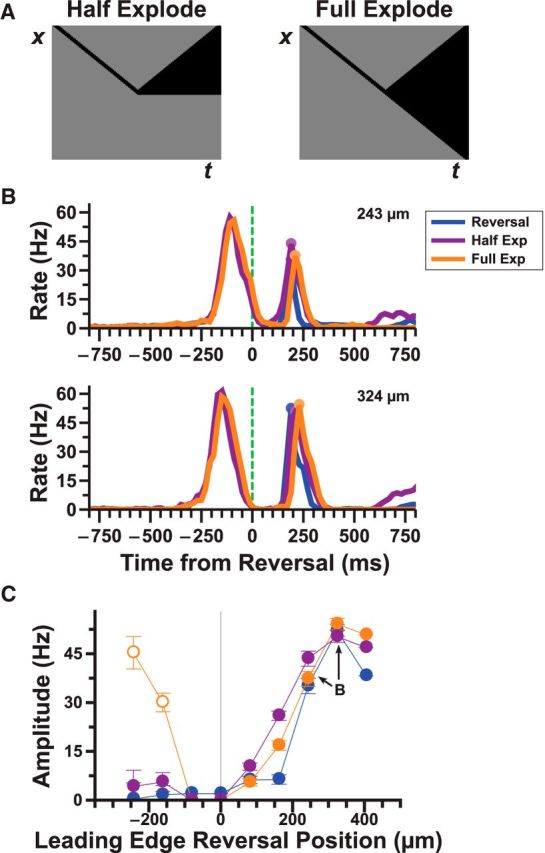
Pure OFF stimuli can also produce a reversal response. A, Pictogram of the half and full explode stimuli. B, Responses of 14 reversal responsive fast OFF cells to reversal (blue), half (purple), and full (orange) explode stimuli. C, Amplitude of the reversal responses to the three different stimuli shown in B given different reversal/explode positions. For very negative positions, as the leading edge of the full explode stimulus continues to move in smooth motion, it also produces a response during the window used to detect reversal responses. These false positives are designated with open circles.

Blockers of inhibitory neurotransmission do not abolish the reversal response

To test what role inhibitory signaling might have in generating the reversal response, we blocked chemical inhibition using a mixture of pharmacological agents (bicuculline for GABA_A receptors, picrotoxin for GABA_A and GABA_C receptors, and strychnine for glycine receptors). As expected, blocking inhibition resulted in an increase in firing rate throughout the retina (average firing rate across fast OFF cells before drug was 10.9 ± 1.3 Hz; after blockers of inhibition, it was 16.0 ± 2.9 Hz.) Additionally, the smooth motion responses occurred earlier in the presence of drugs, evidence of a disruption in the circuitry of the receptive field surrounds (Fig. 4A). As for motion reversal, we found that the reversal response was largely unaffected (Fig. 4A), suggesting that amacrine cells do not play a major role in this computation. Additionally, contrast adaptation has also been shown to be unaffected by blockers of inhibition, suggesting that these adaptive mechanisms may also play a role in generating the reversal response (Garvert and Gollisch, 2013).

The input currents to ganglion cells are reversal responsive

To investigate the roles of synaptic excitation and inhibition in driving the ganglion cell reversal response, we measured the input currents to ganglion cells in a whole-mount retina while stimulating with reversing bars (see Materials and Methods). From these recordings, we found excitatory currents that also responded to motion reversal with a peak of fixed latency with respect to motion reversal of both edges (Fig. 5A, bottom) and bars (Fig. 5C, middle). These currents were also well correlated with the spiking patterns of the cell (Fig. 5C, bottom). Inhibitory currents were also observed, but these currents were often of much smaller amplitude than the excitatory currents, did not exhibit a constant latency as a function of reversal position, and did not prevent the cell from spiking when both currents were present at the same time (Fig. 5C). Interestingly, the cell shown in Figure 5C did not exhibit a noticeable smooth motion response, suggesting that it only responded to reversal. This was found in a small minority of the ganglion cells from which we recorded (<10 of ∼600).

Figure 5.

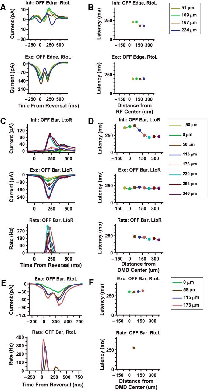
Excitatory currents to ganglion cells are reversal responsive and largely excitatory. A, Inhibitory (top) and excitatory (bottom) currents recorded from a ganglion cell in response to a reversing edge. B, Latency of the reversal responses for different reversal locations. C, Inhibitory (top) and excitatory (middle) currents, along with firing rate (bottom) recorded from a ganglion cell in response to a reversing bar. D, Latency of the reversal responses for different reversal locations. E, Excitatory current (top) and firing rate (bottom) recorded from a ganglion cell in response to a reversing bar. F, Latency of the reversal responses for different reversal locations.

The dominance of the excitatory currents during the reversal response suggests that this response is primarily driven by excitation from bipolar cells. The conclusion we draw from these data is that, when we formulate a minimal computational model, we should first attempt models that include bipolar cells but leave out explicit terms for amacrine cells. Amacrine cells do form inhibitory synapses onto bipolar cell terminals (Dowling and Werblin, 1969; Burkhardt, 1972; Werblin et al., 1988; Dong and Werblin, 1998; Roska et al., 1998), and we cannot rule out the possibility of disinhibition in the amacrine cell circuitry contributing to the generation of the excitatory current that we measure. However, these effects can be captured by a phenomenological gain control mechanism in individual bipolar cells, which we do include in our computational model.

Additionally, evidence for gain control at the ganglion cell level can be seen in looking at the responses of the non-reversal responsive cell (Fig. 5E). The excitatory currents into the cell show a larger second response to motion reversal (Fig. 5E, top); however, the cell only exhibits a response to smooth motion (Fig. 5E, bottom). As inhibitory currents do not appear to play a significant role in modulating the reversal response (Figs. 4 and 5C), this suggests a process inherent to the ganglion cell (i.e., gain control).

A computational model of retinal responses to motion reversal

Previous work has shown that the linear–nonlinear (LN) model as well as the LN model with gain control fail to reproduce the reversal response (Schwartz et al., 2007). However, we recently developed a model that includes rectified subunits in the ganglion cell receptive field as well as gain control mechanisms in both the bipolar and ganglion cells. The bipolar gain control most likely represents the combined effects of many different gain control mechanisms: ion channel inactivation, synaptic depression, receptor desensitization, and inhibitory feedback from amacrine cells (Mennerick and Matthews, 1996; Burrone and Lagnado, 2000; Singer and Diamond, 2006). The ganglion cell gain control also represents a combination of intrinsic mechanisms (Lukasiewicz and Werblin, 1988; Kim and Rieke, 2003) and amacrine cell feedforward inhibition (Russell and Werblin, 2010; Werblin, 2011). This adaptive cascade model (ACM) was able to describe the transient burst of ganglion cell firing following the sudden onset of motion (Chen et al., 2013). We reasoned that this model might also be able to describe the response to motion reversal, which is another form of motion discontinuity.

One source of complexity in formulating a computational model is the diversity of reversal selectivity within the ganglion cell population. Spurred by the observation that some ganglion cells were able to be reversal responsive to both bars and edges, our strategy was to first construct a model that could generate a reversal response in both of these conditions. We reasoned that it would be simpler to first create a model that could be used for both bars and edges, and then see how it could be modified to produce reversal-specific responses, rather than trying to construct separate models for reversal responses to bars and edges and then combining them together. As mentioned previously, we only attempted to model the responses of reversal responsive fast OFF cells to moving dark objects.

As both the ON and OFF pathways were found to be required for responding to reversing edges and bars, we incorporated ON bipolar cells into the ACM. For simplicity, the ON bipolar cells in our model were identical to the OFF bipolar cells, with the exception that the temporal kernel was of opposite polarity (Fig. 6A). In reality, ON and OFF bipolar cells have different gain control properties, with OFF bipolar cells undergoing greater changes in gain and temporal processing during contrast adaptation (Chander and Chichilnisky, 2001; Rieke, 2001; Beaudoin et al., 2008). However, adding separate gain control parameters for ON and OFF bipolar cells would add several more parameters to the model, increasing its complexity.

Figure 6.

The ACM captures the reversal response. A, Schematic illustration of the ACM with ON and OFF bipolar cells. B, Top, Model responses to a dark bar that reverses at a position 243 μm past the RF center (light blue) as well as for a bar in smooth motion (pink) for two different speeds (1.62 mm/s left, and 0.81 mm/s right). Population average firing rate for fast OFF ganglion cells responding to motion reversal (blue) and smooth motion (red). Bottom, Time-varying gain of the model ganglion cell responding to motion reversal (light blue) and smooth motion (pink).

In ∼25% of salamander ganglion cells, crossover inhibition has been shown to link the ON and OFF pathways (Pang et al., 2007). But because blocking inhibition did not seem to affect the reversal response (Fig. 4), we did not include any such mechanism in our model. Fast OFF cells receive stronger input from the OFF pathway (Geffen et al., 2007; Gollisch and Meister, 2008); and to account for this imbalance, we weighted the ON pathway by a factor ϕ = 0.15 less than the OFF pathway when combined at the level of the ganglion cell (see Materials and Methods). To combine inputs across spatial locations, the model assumed identical ON and OFF bipolar cells on the same spatial lattice and then performing a sum weighted by the spatial profile of the ganglion cell receptive field (Chen et al., 2013).

We fit the ACM simultaneously to smooth motion and motion reversal of a dark bar and found that it was able to capture both responses quite well (Figs. 6B and 7A). In particular, the model was able to reproduce the fixed latency of the response over multiple reversal positions, a key characteristic of a reversal response (Fig. 7D, bottom). Additionally, the model reproduced the variation of the peak amplitude of the reversal response as a function of reversal location for all stimuli tested (Fig. 7D–F, top). When we applied the model to both kinds of exploding bar stimuli, we also found good agreement (Fig. 7B,C).

Figure 7.

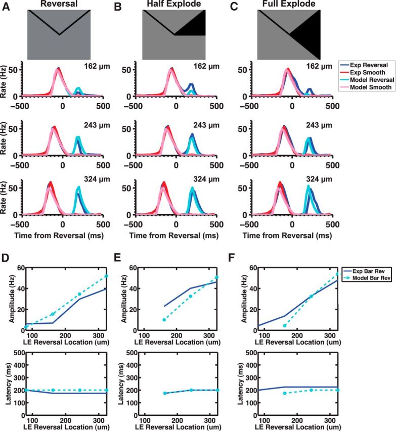
ACM simulations of motion reversal. A, B, C, Model simulations of the response to three different stimuli: reversal (A), half explode (B), and full explode (C). D, E, F, Comparison of the model's (light blue) reversal response amplitude (top) and latency (bottom) to the experimental (blue) reversal (D), half explode (E), and full explode (F) responses.

In the case of reversing edges, we found that the ON pathway was required for the reversal response. To test whether this was also true for the ACM, we simulated the effects of L-AP4 on the model by eliminating the contribution from the ON pathway (i.e., setting ϕ = 0). As in our experimental observations, the ACM did not produce a reversal response when the input from the ON pathway was eliminated (Fig. 8A, left, B, left, C, right). Additionally, the ACM was consistent with our experimental findings that blocking the ON pathway eliminated the reversal response of a dark bar at positions where the leading edge triggered the reversal response (Fig. 8B, right).

Figure 8.

ACM simulation of L-AP4 on motion reversal. A, B, Model simulations of the effect of L-AP4 on the responses to reversing bars (right) and edges (left) at two different distances past the cell's RF center, 81 μm (A) and 243 μm (B). C, Comparison of the model's reversal response amplitude for before (left) and during L-AP4 application (right). Blue represents reversal responses to bars; green represents responses to edge. Pictograms: OFF stimuli (purple), ON stimuli (green).

How does the ACM account for the motion reversal response?

The ACM is a complex model with many dynamical variables. To gain insight into its properties and better understand how it can account for the motion reversal response, it is helpful to investigate its internal variables. The membrane voltage on a bipolar cell, V_i(t), is given by a convolution of the cell's classical, center-surround receptive field with the visual stimulus. For a bar moving at constant velocity, this initially produces mild inhibition due to the surround, followed by strong excitation when the bar hits the receptive field center, and finally a prolonged inhibition (Fig. 9A, blue). This trailing inhibition is primarily due to the biphasic nature of the impulse kernel, not the surround, as can be verified by recalculating with a monophasic impulse kernel (data not shown). The nonlinear function truncates negative values to produce N_i(t) (Fig. 9A, green). The gain control is strong, so that the gain, G_i(t), rapidly drops to zero as the cell is activated by motion on its center (Fig. 9A, yellow). This causes the net output of the bipolar cell, R_i(t), to be relatively transient relative to the linear response (Fig. 9A, red vs blue).

Figure 9.

Understanding the internal variables of the ACM. A, Response of a bipolar cell at x_i = 0 μm to smooth motion: linear response V_i(t) (blue), nonlinear response N_i(t) (green), time-dependent gain G_i(t) (yellow), and gain control output R_i(t) (red). B, Top, Response of the bipolar cell array to motion reversal at x = 180 μm for (i) linear response, (ii) nonlinear response, and (iii) gain control output. Rows represent bipolar cells with centers at different locations; response amplitude shown by color scale. Bottom, Response variables weighted by the spatial profile of synaptic weights, w_i. C, Response of a bipolar cell at x_i = 0 μm to motion reversal at x = 180 μm: linear response V_i(t) (blue), nonlinear response N_i(t) (green), time-dependent gain G_i(t) (yellow), and gain control output R_i(t) (red). D, Top, Ganglion cell activity, A_G(t). Middle, Ganglion cell gain, G_G(t). Bottom, Ganglion cell firing rate, R_G(t).

The response of a bipolar cell to a smoothly moving object has translation invariance, so that the response of every cell is identical up to a time shift related to when the object enters its receptive field. For motion reversal, this invariance is broken, and we need to visualize the response of the entire bipolar cell array across time (Fig. 9B). For bipolar cells far from the location of motion reversal, the response consists of two episodes similar to that for smooth motion: one for motion in the original direction and the other for motion after reversal (Fig. 9Bi, x_i ≤ −200 μm). For bipolar cells closer to the reversal location, the two peaks of excitation merge into one peak (Fig. 9Bi, 0 μm < x_i ≤ 100 μm). We can envision how these responses would combine together at the level of the ganglion cell by constructing what we call the “linear response” of the ganglion cell, R_linear(t) = ${\displaystyle {\sum }_i{w}_i{V}_i\left(t\right)}$, which is simply a sum of the responses of all bipolar cell somas weighted by their synaptic couplings to the ganglion cell, w_i. This function has one peak due to smooth motion and a second peak triggered by motion reversal; the second peak is smaller due to lingering inhibition. This function, R_linear(t), does not directly appear anywhere in the ACM; here, we calculate it for illustrative purposes.

Next, we follow the nonlinear response of bipolar cells, N_i(t). This non-negative response traces the motion of the bar (Fig. 9Bii). Immediately after motion reversal, the peak of the nonlinear response is reduced, again due to lingering inhibition. When we calculate the “nonlinear response” of the ganglion cell, R_nonlin(t) = ${\displaystyle {\sum }_i{w}_i{N}_i\left(t\right)}$, we find that the second peak is diminished in amplitude, primarily because the loss of inhibition has reduced the “sharpening” of the response following motion reversal. However, the gain control mechanism produces a more transient output from each bipolar cell, R_i(t), such that a distinct peak of activity following motion reversal emerges in the ganglion cell soma voltage, V_G(t) = ${\displaystyle {\sum }_i{w}_i{R}_i\left(t\right)}$. Importantly, the time period required for bipolar cells to recover their gain after the first pass of the moving bar results in a “gap” in responses immediately following reversal (Fig. 9Biii), which reduces the ganglion cell voltage V_G(t) almost to zero after the reversal. This gap can be seen more clearly in the response of a single bipolar cell, where the gain remains close to zero during the second peak of excitation in the soma voltage, such that the output of the cell has only a single peak (Fig. 9C).

Finally, the action of the ganglion cell gain control serves to accentuate the peak of activity following motion reversal (Fig. 9D). The activity variable, A_G(t), which is a smoothed version of the soma voltage V_G(t), sets the time-varying gain. The ganglion cell's gain is significantly reduced during smooth motion, which truncates the response earlier and shifts its peak to earlier times, as seen in a previous study of motion anticipation (Berry et al., 1999). Then, the gap in bipolar cell activity allows the gain to recover somewhat before the excitation triggered by motion in the new direction, thus resulting in a larger peak in the ganglion cell's firing rate.

Emergence of a fixed latency response in the ACM

A key characteristic of the reversal response is the fixed latency of the peak in the firing rate after motion reversal at different locations. This property is significant for the neural code because it gives rise to a precise synchronization of the firing of many ganglion cells distributed over a wide spatial range, which in turn allows the brain to distinguish motion reversal from smooth motion (Schwartz et al., 2007). We wanted to understand how the ACM actually achieved a fixed latency response because it was not transparent how this property was represented by the model's structure or by any of its parameter values. Because ON and OFF pathways were both active during the response to reversing bars, we focused instead on the simpler case of the “half-exploding bar” stimulus, where only the OFF pathway operates. A similar analysis of the combined responses of ON and OFF pathways operative during reversal of a bar revealed the same qualitative picture (data not shown).

The basic mechanism is illustrated schematically in Figure 10A. After the moving bar passes over a bipolar cell, that cell has its gain strongly suppressed, rendering it unresponsive. Therefore, after motion reversal, the bar will not generate bipolar responses until after a characteristic time τ has elapsed. For reversal at one location, the moving bar will trigger responses from one small group of bipolar cells. For another location, the bar will trigger responses from a different group of bipolar cells, but the response will again occur at a time τ after reversal.

Figure 10.

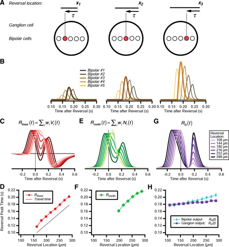
Emergence of a fixed latency response to motion reversal. A, Top, Motion reversal a three different reversal locations: x₁, x₂, and x₃. Bottom, Ganglion cell (large circle) with multiple bipolar cells within its receptive field (smaller circles). At different reversal locations, a different bipolar cell is responsive (red). B, Response of five different bipolar cells in the ACM; bipolar cells are spaced by 27 μm, and their identity is indicated by color. Responses are scaled by the synaptic weight of each bipolar cell, w_i, to reflect its relative contribution to excitation of the ganglion cell. C, Linear response, R_linear(t), shown for six different reversal locations, indicated by hue. D, Latency of the peak in the linear response following motion reversal (red). Shown for comparison is the time at which the trailing edge of the bar reaches the receptive field center coordinate, plus a 100 ms delay (dashed line). E, Nonlinear response, R_nonlin(t), for the same six reversal locations, indicated by hue. F, Latency of the peak in the nonlinear response following motion reversal (green). G, Ganglion cell firing rate for the same six reversal locations, indicated by hue. H, Latency of the peak ganglion cell voltage V_G(t) (blue diamonds) and ganglion cell firing rate R_G(t) (purple squares) following motion reversal.

Of course, this schematic illustration is an overly simplified picture. When we examine the activity of different bipolar cells in the ACM, we find that there is a more continuous distribution of responses across space and time. However, for reversals at different locations, different bipolar cells have the largest response (Fig. 10B). Furthermore, the largest response has a peak value at nearly the same time across the different reversal locations (Fig. 10B).

We can appreciate that this constancy of the reversal response's latency does not trivially emerge from simpler functional models by examining the different processing stages of the ACM. When we construct the linear response, R_linear(t), we find that the peak in excitation following motion reversal shifts linearly as a function of the reversal location (Fig. 10C,D). This is consistent with the time required for the moving bar to return to the same position on the receptive field following motion reversal (Fig. 10D, dashed line). Furthermore, for some reversal locations, the excitation triggered by motion in the new direction merges with excitation triggered by motion before reversal, such that there is no peak associated with motion reversal at all. Bipolar cell nonlinearity does not change this picture, as R_nonlin(t) also shifts approximately linearly as a function of reversal location (Fig. 10E,F).

Instead, gain control mechanisms play a major role in establishing the constancy of reversal response latency. Because the bipolar cell gain recovers abruptly after its intrinsic time τ_B has elapsed (Fig. 10C), the response latency of the ganglion cell voltage, V_G(t), is more constant versus reversal location (Fig. 10H, light blue). The ganglion cell gain control also plays a role, as seen by the fact that the latency of the peak in the ganglion cell's firing rate is even more constant (Fig. 10G,H). Again, strong activation by the bar moving in the original direction suppresses the ganglion cell's gain, which requires at least a time τ_G to recover, thus imposing another source of delay before the peak firing rate is achieved.

Sensitivity of the ACM to individual parameters

Because the fixed latency of the reversal response appears to arise from a combination of both bipolar and ganglion cell gain control functions, we sought to characterize how each individual parameter affected the output of the model. This was achieved by manipulating a single parameter, while fixing all the other ones at their original values. As expected, when we increased the time constant of the bipolar cell gain control, τ_B, we saw as monotonic shift toward longer reversal response latencies (Fig. 11A). This occurs because the reversal response cannot be generated until bipolar cells recover their gain, and a longer τ_B means that it takes longer for their gain to recover. This was a significant effect, shifting the latency by up to ∼100 ms. Note, however, that the simple picture of bipolar cells needing to wait until their gain recovers does not account the nonlinear dependence of latency on τ_B; instead, this property emerges from the nonlinear interactions of the full model. A qualitatively similar effect was apparent for variations of τ_G (Fig. 11A). But because the latency of the reversal response was primarily controlled by the recovery of bipolar cell gain, τ_G had much less effect on the latency. Both time constants had a strong effect on the amplitude of the reversal response, measured here as a ratio of the peak firing rate following motion reversal to the peak firing rate during smooth motion (Fig. 11B). This occurs because a longer time constant allows for the activity variables, A_B and A_G, to build up to larger values, thereby suppressing the gain by larger factors.

Figure 11.

Sensitivity of the reversal response to parameters of the ACM. A, Peak latency of the reversal response in the ACM as a function of the two time constants, τ_B (triangles) and τ_G (open circles). B, Ratio of the peak firing rate following motion reversal versus the peak firing rate for smooth motion in the ACM plotted as a function of the two time constants, τ_B (triangles) and τ_G (open circles). C, Peak latency of the reversal response in the ACM as a function of the two gain control amplitudes, H_B (triangles) and H_G (open circles); their values in the ACM matched to data are denoted as H_B0 and H_G0, respectively. D, Ratio of the peak firing rate following motion reversal versus the peak firing rate for smooth motion in the ACM plotted as a function of the two gain control amplitudes, H_B (triangles) and H_G (open circles). All data shown for a reversal at x = 234 μm past the receptive field center; results were strongly invariant to the reversal location.

Variation of the bipolar cell gain control amplitude, H_B, had an effect qualitatively similar to that for the time constant, τ_B: the reversal peak latency increased for larger H_B, as a stronger gain control meant that more time was required for the gain to recover to a criterion value (Fig. 11C), and the reversal peak amplitude decreased (Fig. 11D). Variation of the ganglion cell gain control amplitude, H_G, was different. Here, the influence on the reversal peak latency was dominated by the “anticipation effect” (Berry et al., 1999): namely, that a stronger gain control mechanism truncated the ganglion cell's firing rate more quickly, thereby shifting the peak of activity to an earlier time (Fig. 11C). The amplitude of the reversal peak was reduced at larger values of H_G; however, this variation had an even stronger effect on the peak response to smooth motion, so that the ratio of the two actually increased (Fig. 11D).

Success of the ACM for a broad class of motion discontinuities

Sudden reversal is just one example from a class of motion discontinuities that have been tested in retinal physiology so far. These tests reveal that the retina responds to a nontrivial set of motion discontinuities, rather than simply signaling acceleration per se (Schwartz et al., 2007). For instance, sudden changes of speed by a factor of two trigger very little specific response. Sudden cessation of motion triggers no response, whereas sudden onset of motion triggers a burst of firing that has a shorter latency and a higher peak rate than motion reversal. Finally, when two bars moving in opposite direction cross, the retina generates a burst of firing that is nearly indistinguishable from the reversal response.

We tested whether the ACM could explain the retinal response to these other kinds of motion discontinuity using the same parameters as were required to explain our measured motion reversal responses. As shown in Figure 12, the adaptive case model was found to be qualitatively consistent with all of these retinal responses. For the case of mild acceleration or deceleration, the gain controls of the model were already engaged by the preceding motion, so there was no clear burst of firing. Interesting, the data as well as the model have a slight uptick in the firing rate following two-fold acceleration; however, this results from simple spatiotemporal integration, namely, the fact that the level of retinal excitation increases at higher speeds. Cessation of motion does not trigger any response because the ACM does not have any dynamical variables that explicitly track or predict motion; hence, there are no terms for “negative acceleration.” However, the onset of motion triggers a response bigger than for reversal because retinal gain controls are able to achieve their maximum values beforehand. Finally, the case of crossing bars is interesting because the movement pattern seen by the retina in a hemifield on one side of the motion reversal is the same as for the crossing bars. The similarity in retinal responses implies that the mechanism that generates the reversal response is relatively local in space, as is the case for the structure of the ACM. The qualitative agreement with this diverse set of motion discontinuity data further strengthens our confidence in the ACM.

Figure 12.

Testing the ACM for different kinds of motion discontinuities. A, Ganglion cell firing rate predicted by the ACM for sudden two-fold deceleration (top), smooth motion (middle), and sudden two-fold acceleration (bottom). Speed beforehand was 1.62 mm/s; accelerations occurred at a position x = 0 on the receptive field center. B, Population firing rate predicted by the ACM for motion reversal (top), sudden cessation of motion (middle), and sudden onset of motion (bottom). For consistency with published experimental data, firing rates were averaged over a set of locations triggering a reversal response for top and middle (x = 108–288 μm in steps of 36 μm) and triggering a motion onset response for bottom (x = 0, ±90 μm, ±180 μm). C, Population firing rate predicted by the ACM for smooth motion (top), a reversing bar (middle), and a pair of crossing bars (bottom); responses were averaged across a set of locations triggering a reversal response (x = 108–288 μm in steps of 36 μm).

Selectivity for motion reversal

The basic mechanism underlying the motion reversal response is the reexcitation of bipolar cells after they recover their gain. This raises the question: can a similar response be triggered by a second bar moving in tandem behind the first bar? We addressed this question by performing experiments with two bars moving at the same velocity but separated by a spatial gap. We found that the second bar generated a ganglion cell response that grew and peaked at later times as the spacing between the two bars increased (Fig. 13A). Using the ACM with the same parameters as before, we found a ganglion cell response that was qualitatively very similar (Fig. 13B). The time to peak of this response scaled approximately linearly with the spatial gap between the two bars (Fig. 13C). This is the behavior one expects for the second bar simply encountering the ganglion cells' receptive fields (Fig. 13C, dashed line). Thus, this response will not be synchronized among a distributed population of ganglion cells, as is true for the motion reversal response. The effect of gain control was clearly evident, both in the diminished peak amplitude for small gaps between the bars (Fig. 13A) and in the increased latency for small gaps (Fig. 13C), but there was nothing special about the timing of this response.

Figure 13.

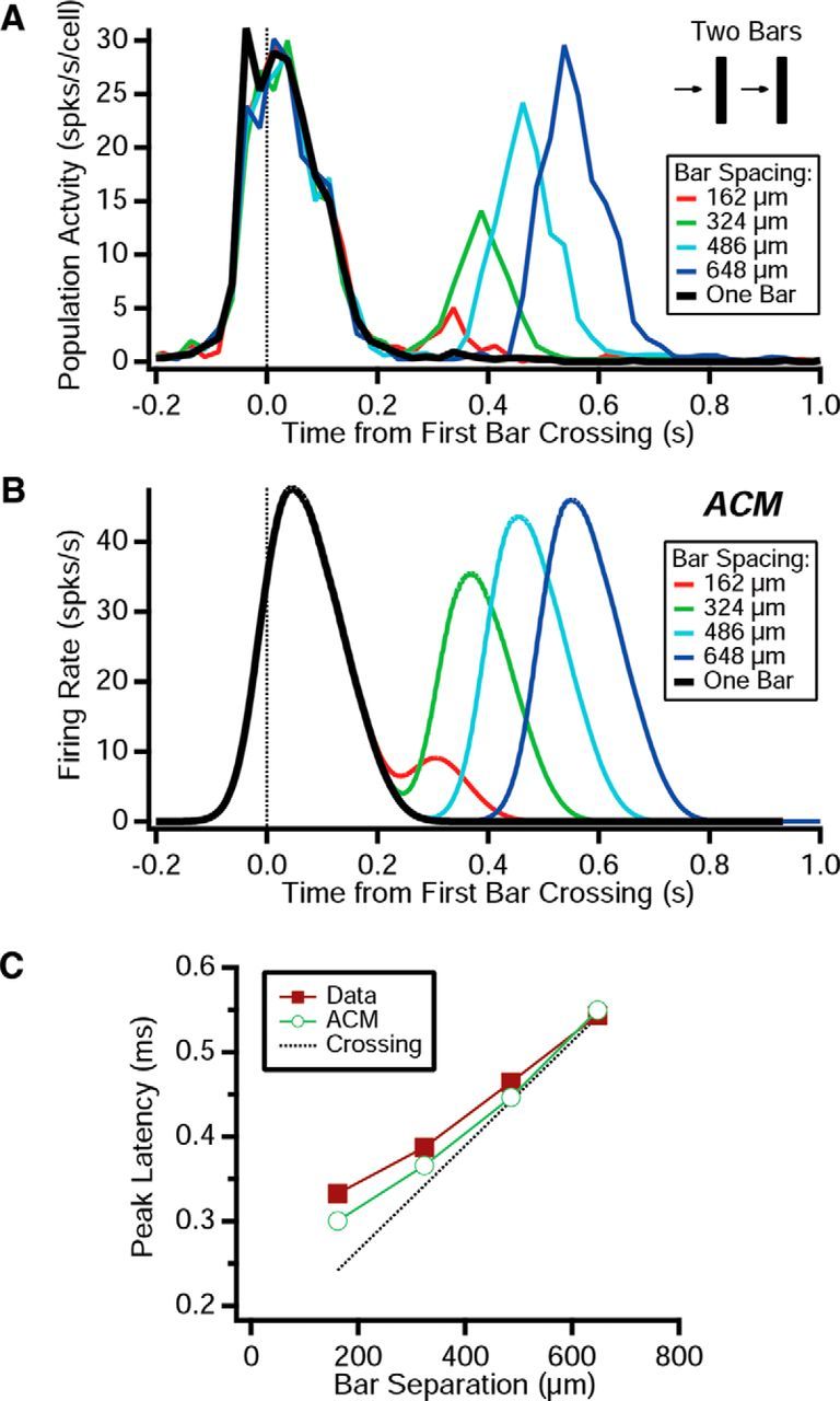
Specificity of the reversal response. A, Population average firing rate responding to two bars moving in the same direction plotted versus time at which the leading edge of the first bar crosses the RF center. B, ACM firing rate responding to two bars moving in the same direction plotted versus time at which the leading edge of the first bar crosses the RF center. C, Latency of the response to the second bar plotted versus the spatial gap between the two bars for experimental data (squares), ACM (open circles); also shown is the latency predicted by the time of the second bar crossing the RF center (dashed line).

The motion reversal response for dark edges

We have seen above that the response to reversal of a dark edge is blocked entirely by APB, implying that the ON pathway alone generates this response. Consequently, the mechanism we have described above, which generates a synchronized motion reversal response via the coordinated recovery of the gain of bipolar cells, cannot explain this kind of motion reversal response. At the same time, we have seen that the full ACM, including both ON and OFF pathways, does match the time-varying firing rate of fast OFF cells responding to the reversal of a dark edge, both with and without APB (Fig. 8). So how does the ACM generate this kind of motion reversal response? And why is the latency constant as a function of reversal location?

We first examined the role of the ON pathway in the ACM. When the dark edge reversed, individual ON bipolar cells had a linear response that was strongly inhibited by the edge's motion before and just after reversal, and then swung sharply to excitation after the edge retreated off of the bipolar cell's receptive field (Fig. 14A, blue lines). Across the array of bipolar cells, the latency of the excitatory response was relatively constant. The reason was that different ON bipolar cells reached a saturated level of inhibition that was approximately constant across cells. As a result, an approximately similar amount of time was required to overcome this inhibition. Consequently, the output of different bipolar cells had a peak that was relatively constant (Fig. 14A, red lines).

Figure 14.

The reversal response for dark edges. A, B, Response of three different (ON, OFF) bipolar cells to a dark edge that reverses at location x = 0; bipolar cell soma voltage, V_i(t) (blue); bipolar output, R_i(t) (red); time of the peak reversal response (pink arrow). C, Ganglion cell firing rate for four different reversal locations, indicated by hue. D, Latency of the peak ganglion cell firing rate, R_G(t), following reversal of a dark edge (orange diamonds) or a dark bar (purple squares); dashed line indicates travel time.

As expected, OFF bipolar cells were excited by the smooth motion of the dark edge before reversal and did not have any significant excitation after reversal (Fig. 14B). As a result, the OFF pathway generated the smooth motion response before reversal, and the ON pathway generated the peak in the firing rate after reversal. Putting these results together across, the ganglion cell's firing rate had a peak following motion reversal that was nearly constant across different reversal locations (Fig. 14C). In contrast, the initial peak in the firing rate was due to smooth motion that shifted systematically with reversal locations. Although the latency of the reversal response did shift systematically with reversal location, this shift was much smaller than would be expected for a response triggered by the edge traveling back to a criterion location (Fig. 14D).

Although the peak in firing after reversal of a dark edge resembled that for a dark bar, there are important differences between them. First, the absolute latency of the response to the edge was longer than for the bar (Fig. 14D); this difference was also observed in the experimental data: latency = 205 ± 2.4 ms (SE) for the edge and 194 ± 2.6 ms for the bar (p = 0.001). More importantly, the mechanisms responsible for these synchronized responses were qualitatively different: for reversal of an edge, constant latency across reversal locations was a consequence of the recovery from a saturating level of inhibition, whereas for a bar, constant latency emerged from the recovery of bipolar cell gain. Given these different mechanisms, it is perhaps no surprise that the existence of reversal responses for these two kinds of stimuli was independently distributed within the ganglion cell population (Tables 2 and 3).

Discussion

In exploring the circuit mechanism underlying the response to motion reversal, we first found that selectivity for multiple kinds of objects was randomly distributed in the ganglion cell population, suggesting that the retina contains multiple, parallel circuits to compute motion reversal. Using pharmacology and designed stimuli, we found that motion reversal can be elicited from a mechanism dependent on the ON pathway (for the cases of reversal of a dark edge or the leading edge of a dark bar) or a mechanism independent of the ON pathway (for the trailing edge of a dark bar or “exploding bar” stimuli). Using pharmacology and patch-clamp recording, we found that inhibition did not play a major role in generating the reversal response.

Bringing these observations together, we formulated a version of the ACM, previously used to describe the ganglion cell response to motion onset. This model involves nonlinear subunits in the ganglion cell's receptive field, interpreted to be individual bipolar cells. Crucially, the model includes mechanisms of gain control at both the bipolar cell and ganglion cell levels, a structure that has also been implicated in contrast adaptation (Garvert and Gollisch, 2013). By incorporating ON bipolar cells into the ACM, we were able to account for our experimental results, not only for reversing bars and edges with and without L-AP4, but also for a broad set of motion stimuli: exploding bars, two-fold changes in speed, sudden onset of motion, sudden cessation of motion, crossing bars, and two bars moving in tandem.

The basic picture that emerges is that the motion reversal response can be generated by two different mechanisms. Within the OFF pathway, the reversal response is primarily caused by reexcitation of bipolar cells. The reversal response is relatively sharp and transient because the relevant bipolar cells were stimulated by the period of smooth motion before the reversal and, hence, need to recover their full gain. Given the parameters in the ACM that best fit our data, this recovery of gain was relatively sudden in time, leading to a transient response synchronized across different ganglion cells. Within the ON pathway, a synchronized reversal response results from recovery from a saturating level of preceding inhibition. Because either ON or OFF bipolar cells could generate a motion reversal response, the ability to respond to the reversal of different kinds of moving objects was distributed independently within the ganglion cell population.

Consistent with this picture for the OFF pathway, the constant latency of the response as a function of different reversal locations was strongly affected by the time constant of bipolar cell gain control, τ_B, but only weakly affected by the time constant of ganglion cell gain control, τ_G. However, all of the processing stages of the ACM contributed in different ways to shaping and enhancing the peak in the firing rate triggered by motion reversal. This illustrates the value of formulating explicit computation models: such models can sometimes have advantageous properties that were difficult to intuit from their individual ingredients.

Multiple neural circuits for computing motion reversals

One of the major surprises in this study was the finding that different subsets of ganglion cells generated responses to the reversal of different kinds of moving objects. Why might the retina want to have these circuits connect randomly to different ganglion cells, instead of building reversal detectors that are invariant to the spatial details of the object that is reversing?

One obvious speculation is that this kind of population neural code can explicitly represent not just the fact that there is motion reversal at a particular location in space, but also the kind of object that is reversing. Our bar stimuli were objects whose size was smaller than the ganglion cell receptive field, whereas our edges were like objects with a size much larger than the receptive field. In general, an animal might want to activate categorically different behaviors upon observing these two kinds of moving objects: for instance, the salamander might want to snap at a small object but initiate an escape response for a very large object (Ishikane et al., 2005).

Of course, the entire population of retinal ganglion cells represents the difference between large and small moving objects with a spatial map, where different groups of ganglion cells respond to the leading and trailing edges of a large object. Then, higher visual centers can combine this information to recognize the motion of the large object. However, having this information explicitly represented at the level of a local population code allows these behavioral decisions to be computed faster and using shorter sensory–motor pathways. What is the limit of this representation of object category? Ewert and colleagues have shown that the toad generates different behaviors and visual responses for elongated moving objects (‘worms’) versus objects moving at right angles to their long axis (“anti-worms” or “bars”) (Tsai et al., 1983; Ewert, 1997). Given that approximately one-third of all of the ganglion cells are reversal responsive, there is significant capacity to explicitly represent more than just big/small and light/dark reversing objects.

Different kinds of motion discontinuities

Because we could explain the motion reversal response with the same computational model used to explain the response to motion onset, it is natural to think of these retinal computations as being quite similar. In both cases, there is a sudden discontinuity of motion and a transient burst of ganglion cell firing. Perhaps, on a conceptual level, we might like to think of motion reversal as the “onset” of motion in a new direction. In any case, if the retina is making some prediction of the location of the object given its current trajectory, then this prediction will break down immediately following any change in direction. Although simulations of object tracking have shown that the tracking of an object's position can recover relatively quickly (Leonardo and Meister, 2013), certain instances where the retina's prediction has critically failed, such as in motion onset and motion reversal, may nevertheless be salient enough to warrant encoding (by the retina). Thus, both the motion onset and reversal responses might be thought of an “alert” that the brain might use to reset more central motion extrapolation mechanisms as well as initiate changes in attention.

In this context, motion onset has been shown to be a salient stimulus (Abrams and Christ, 2003; Christ and Abrams, 2008), but what about motion reversal? Similar to motion onset, motion reversal evokes a characteristic visual-evoked potential in humans (MacKay and Rietveld, 1968; Clarke, 1973). Additionally, catch-up saccades can be triggered by large errors in smooth pursuit eye movements (Robinson, 1965; Friedman et al., 1991; de Brouwer et al., 2002; Medina et al., 2005; Voss et al., 2007), although these saccades are not limited only to reversals. Interestingly, motion offset does not capture attention (Abrams and Christ, 2003), consistent with the fact that this stimulus causes no extra retinal firing.

Nevertheless, although salient stimuli such as object appearance and motion onset produce high rates of firing from ganglion cells, the amplitude of the reversal response is rarely larger than the response to smooth motion. If one were only considering the firing rates of individual ganglion cells as a measure of saliency, then motion reversal would not be considered salient in the context of the informal “salience ranking” proposed by Christ and Abrams (2008). However, motion reversal triggers strongly synchronized retinal firing, which indeed allows reversal to be unambiguously distinguished from smooth motion (Schwartz et al., 2007).

Synchronous activity among neurons has been proposed to increase saliency (Singer and Gray, 1995), and oscillatory synchrony per se in the retina appears to drive an escape response from looming visual stimuli in the frog (Ishikane et al., 2005). More specifically, transient visual responses in the superior colliculus have been involved with generating a “priority” signal to an event, and also sometimes in the generation of an express saccade (Boehnke and Munoz, 2008). Although it is not known whether motion reversals or onsets can trigger these collicular responses, it is plausible that transient visual responses are driven by these particular stimuli, thus linking the retinal code (transient, synchronous responses) with a behavioral manifestation of salience (an express saccade).

References

- Abrams RA, Christ SE. Motion onset captures attention. Psychol Sci. 2003;14:427–432. doi: 10.1111/1467-9280.01458. [DOI] [PubMed] [Google Scholar]
- Baccus SA, Olveczky BP, Manu M, Meister M. A retinal circuit that computes object motion. J Neurosci. 2008;28:6807–6817. doi: 10.1523/JNEUROSCI.4206-07.2008. [DOI] [PMC free article] [PubMed] [Google Scholar]
- Beaudoin DL, Manookin MB, Demb JB. Distinct expressions of contrast gain control in parallel synaptic pathways converging on a retinal ganglion cell. J Physiol. 2008;586:5487–5502. doi: 10.1113/jphysiol.2008.156224. [DOI] [PMC free article] [PubMed] [Google Scholar]
- Berry MJ, 2nd, Brivanlou IH, Jordan TA, Meister M. Anticipation of moving stimuli by the retina. Nature. 1999;398:334–338. doi: 10.1038/18678. [DOI] [PubMed] [Google Scholar]
- Boehnke SE, Munoz DP. On the importance of the transient visual response in the superior colliculus. Curr Opin Neurobiol. 2008;18:544–551. doi: 10.1016/j.conb.2008.11.004. [DOI] [PubMed] [Google Scholar]
- Burkhardt DA. Effects of picrotoxin and strychnine upon electrical-activity of proximal retina. Brain Res. 1972;43:246–249. doi: 10.1016/0006-8993(72)90289-2. [DOI] [PubMed] [Google Scholar]
- Burrone J, Lagnado L. Synaptic depression and the kinetics of exocytosis in retinal bipolar cells. J Neurosci. 2000;20:568–578. doi: 10.1523/JNEUROSCI.20-02-00568.2000. [DOI] [PMC free article] [PubMed] [Google Scholar]
- Chander D, Chichilnisky EJ. Adaptation to temporal contrast in primate and salamander retina. J Neurosci. 2001;21:9904–9916. doi: 10.1523/JNEUROSCI.21-24-09904.2001. [DOI] [PMC free article] [PubMed] [Google Scholar]
- Chen EY, Marre O, Fisher C, Schwartz G, Levy J, da Silveira RA, Berry MJ., 2nd Alert response to motion onset in the retina. J Neurosci. 2013;33:120–132. doi: 10.1523/JNEUROSCI.3749-12.2013. [DOI] [PMC free article] [PubMed] [Google Scholar]
- Christ SE, Abrams RA. The attentional influence of new objects and new motion. J Vis. 2008;8:21–28. doi: 10.1167/8.3.27. [DOI] [PubMed] [Google Scholar]
- Clarke PG. Comparison of visual evoked potentials to stationary and to moving patterns. Exp Brain Res. 1973;18:156–164. doi: 10.1007/BF00234720. [DOI] [PubMed] [Google Scholar]
- de Brouwer S, Missal M, Barnes G, Lefèvre P. Quantitative analysis of catch-up saccades during sustained pursuit. J Neurophysiol. 2002;87:1772–1780. doi: 10.1152/jn.00621.2001. [DOI] [PubMed] [Google Scholar]
- Dong CJ, Werblin FS. Temporal contrast enhancement via GABA(C) feedback at bipolar terminals in the tiger salamander retina. J Neurophysiol. 1998;79:2171–2180. doi: 10.1152/jn.1998.79.4.2171. [DOI] [PubMed] [Google Scholar]
- Dowling JE, Werblin FS. Organization of retina of the mudpuppy, Necturus maculosus. I. Synaptic structure. J Neurophysiol. 1969;32:315–338. doi: 10.1152/jn.1969.32.3.315. [DOI] [PubMed] [Google Scholar]
- Ewert JP. Neural correlates of key stimulus and releasing mechanism: a case study and two concepts. Trends Neurosci. 1997;20:332–339. doi: 10.1016/S0166-2236(96)01042-9. [DOI] [PubMed] [Google Scholar]
- Fairhall AL, Burlingame CA, Narasimhan R, Harris RA, Puchalla JL, Berry MJ., 2nd Selectivity for multiple stimulus features in retinal ganglion cells. J Neurophysiol. 2006;96:2724–2738. doi: 10.1152/jn.00995.2005. [DOI] [PubMed] [Google Scholar]
- Friedman L, Jesberger JA, Meltzer HY. A model of smooth pursuit performance illustrates the relationship between gain, catch-up saccade rate, and catch-up saccade amplitude in normal controls and patients with schizophrenia. Biol Psychiatry. 1991;30:537–556. doi: 10.1016/0006-3223(91)90024-G. [DOI] [PubMed] [Google Scholar]
- Garvert MM, Gollisch T. Local and global contrast adaptation in retinal ganglion cells. Neuron. 2013;77:915–928. doi: 10.1016/j.neuron.2012.12.030. [DOI] [PubMed] [Google Scholar]
- Geffen MN, de Vries SE, Meister M. Retinal ganglion cells can rapidly change polarity from Off to On. PLoS Biol. 2007;5:e65. doi: 10.1371/journal.pbio.0050065. [DOI] [PMC free article] [PubMed] [Google Scholar]
- Gollisch T, Meister M. Modeling convergent ON and OFF pathways in the early visual system. Biol Cybern. 2008;99:263–278. doi: 10.1007/s00422-008-0252-y. [DOI] [PMC free article] [PubMed] [Google Scholar]
- Ishikane H, Gangi M, Honda S, Tachibana M. Synchronized retinal oscillations encode essential information for escape behavior in frogs. Nat Neurosci. 2005;8:1087–1095. doi: 10.1038/nn1497. [DOI] [PubMed] [Google Scholar]
- Kim KJ, Rieke F. Slow Na+ inactivation and variance adaptation in salamander retinal ganglion cells. J Neurosci. 2003;23:1506–1516. doi: 10.1523/JNEUROSCI.23-04-01506.2003. [DOI] [PMC free article] [PubMed] [Google Scholar]
- Lennie P, Perry VH. Spatial contrast sensitivity of cells in the lateral geniculate-nucleus of the rat. J Physiol. 1981;315:69–79. doi: 10.1113/jphysiol.1981.sp013733. [DOI] [PMC free article] [PubMed] [Google Scholar]
- Leonardo A, Meister M. Nonlinear dynamics support a linear population code in a retinal target-tracking circuit. J Neurosci. 2013;33:16971–16982. doi: 10.1523/JNEUROSCI.2257-13.2013. [DOI] [PMC free article] [PubMed] [Google Scholar]
- Lukasiewicz P, Werblin F. A slowly inactivating potassium current truncates spike activity in ganglion cells of the tiger salamander retina. J Neurosci. 1988;8:4470–4481. doi: 10.1523/JNEUROSCI.08-12-04470.1988. [DOI] [PMC free article] [PubMed] [Google Scholar]
- Ma J, Znoiko S, Othersen KL, Ryan JC, Das J, Isayama T, Kono M, Oprian DD, Corson DW, Cornwall MC, Cameron DA, Harosi FI, Makino CL, Crouch RK. A visual pigment expressed in both rod and cone photoreceptors. Neuron. 2001;32:451–461. doi: 10.1016/S0896-6273(01)00482-2. [DOI] [PubMed] [Google Scholar]
- MacKay DM, Rietveld WJ. Electroencephalogram potentials evoked by accelerated visual motion. Nature. 1968;217:677–678. doi: 10.1038/217677a0. [DOI] [PubMed] [Google Scholar]
- Makino CL, Taylor WR, Baylor DA. Rapid charge movements and photosensitivity of visual pigments in salamander rods and cones. J Physiol. 1991;442:761–780. doi: 10.1113/jphysiol.1991.sp018818. [DOI] [PMC free article] [PubMed] [Google Scholar]
- Medina JF, Carey MR, Lisberger SG. The representation of time for motor learning. Neuron. 2005;45:157–167. doi: 10.1016/j.neuron.2004.12.017. [DOI] [PubMed] [Google Scholar]
- Mennerick S, Matthews G. Ultrafast exocytosis elicited by calcium current in synaptic terminals of retinal bipolar neurons. Neuron. 1996;17:1241–1249. doi: 10.1016/S0896-6273(00)80254-8. [DOI] [PubMed] [Google Scholar]
- Pang JJ, Gao F, Wu SM. Cross-talk between ON and OFF channels in the salamander retina: indirect bipolar cell inputs to ON-OFF ganglion cells. Vision Res. 2007;47:384–392. doi: 10.1016/j.visres.2006.09.021. [DOI] [PubMed] [Google Scholar]
- Puchalla JL, Schneidman E, Harris RA, Berry MJ. Redundancy in the population code of the retina. Neuron. 2005;46:493–504. doi: 10.1016/j.neuron.2005.03.026. [DOI] [PubMed] [Google Scholar]
- Rieke F. Temporal contrast adaptation in salamander bipolar cells. J Neurosci. 2001;21:9445–9454. doi: 10.1523/JNEUROSCI.21-23-09445.2001. [DOI] [PMC free article] [PubMed] [Google Scholar]
- Robinson DA. The mechanics of human smooth pursuit eye movement. J Physiol. 1965;180:569–591. doi: 10.1113/jphysiol.1965.sp007718. [DOI] [PMC free article] [PubMed] [Google Scholar]
- Roska B, Nemeth E, Werblin FS. Response to change is facilitated by a three-neuron disinhibitory pathway in the tiger salamander retina. J Neurosci. 1998;18:3451–3459. doi: 10.1523/JNEUROSCI.18-09-03451.1998. [DOI] [PMC free article] [PubMed] [Google Scholar]
- Russell TL, Werblin FS. Retinal synaptic pathways underlying the response of the rabbit local edge detector. J Neurophysiol. 2010;103:2757–2769. doi: 10.1152/jn.00987.2009. [DOI] [PMC free article] [PubMed] [Google Scholar]
- Schnapf JL, Kraft TW, Baylor DA. Spectral sensitivity of human cone photoreceptors. Nature. 1987;325:439–441. doi: 10.1038/325439a0. [DOI] [PubMed] [Google Scholar]
- Schwartz G, Taylor S, Fisher C, Harris R, Berry MJ., 2nd Synchronized firing among retinal ganglion cells signals motion reversal. Neuron. 2007;55:958–969. doi: 10.1016/j.neuron.2007.07.042. [DOI] [PMC free article] [PubMed] [Google Scholar]
- Segev R, Puchalla J, Berry MJ., 2nd Functional organization of ganglion cells in the salamander retina. J Neurophysiol. 2006;95:2277–2292. doi: 10.1152/jn.00928.2005. [DOI] [PubMed] [Google Scholar]
- Singer JH, Diamond JS. Vesicle depletion and synaptic depression at a mammalian ribbon synapse. J Neurophysiol. 2006;95:3191–3198. doi: 10.1152/jn.01309.2005. [DOI] [PubMed] [Google Scholar]
- Singer W, Gray CM. Visual feature integration and the temporal correlation hypothesis. Annu Rev Neurosci. 1995;18:555–586. doi: 10.1146/annurev.ne.18.030195.003011. [DOI] [PubMed] [Google Scholar]
- Slaughter MM, Miller RF. 2-Amino-4-phosphonobutyric acid: a new pharmacological tool for retina research. Science. 1981;211:182–185. doi: 10.1126/science.6255566. [DOI] [PubMed] [Google Scholar]
- Soo FS, Schwartz GW, Sadeghi K, Berry MJ., 2nd Fine spatial information represented in a population of retinal ganglion cells. J Neurosci. 2011;31:2145–2155. doi: 10.1523/JNEUROSCI.5129-10.2011. [DOI] [PMC free article] [PubMed] [Google Scholar]
- Tsai H, Burghagen H, Schürg-Pfeiffer E, Ewert JP. Neuronal correlates of edge preference in prey-catching behavior of toads Bufo bufo. Die Naturwissenschaften. 1983;70:310–311. doi: 10.1007/BF00404843. [DOI] [PubMed] [Google Scholar]
- Voss HU, McCandliss BD, Ghajar J, Suh M. A quantitative synchronization model for smooth pursuit target tracking. Biol Cybern. 2007;96:309–322. doi: 10.1007/s00422-006-0116-2. [DOI] [PubMed] [Google Scholar]
- Werblin FS. The retinal hypercircuit: a repeating synaptic interactive motif underlying visual function. J Physiol. 2011;589:3691–3702. doi: 10.1113/jphysiol.2011.210617. [DOI] [PMC free article] [PubMed] [Google Scholar]
- Werblin F, Maguire G, Lukasiewicz P, Eliasof S, Wu SM. Neural interactions mediating the detection of motion in the retina of the tiger salamander. Vis Neurosci. 1988;1:317–329. doi: 10.1017/S0952523800001978. [DOI] [PubMed] [Google Scholar]
- Yang XL. Characterization of receptors for glutamate and GABA in retinal neurons. Prog Neurobiol. 2004;73:127–150. doi: 10.1016/j.pneurobio.2004.04.002. [DOI] [PubMed] [Google Scholar]