Cancer Classification in Microarray Data using a Hybrid Selective Independent Component Analysis and υ-Support Vector Machine Algorithm

Abstract

Microarray data have an important role in identification and classification of the cancer tissues. Having a few samples of microarrays in cancer researches is always one of the most concerns which lead to some problems in designing the classifiers. For this matter, preprocessing gene selection techniques should be utilized before classification to remove the noninformative genes from the microarray data. An appropriate gene selection method can significantly improve the performance of cancer classification. In this paper, we use selective independent component analysis (SICA) for decreasing the dimension of microarray data. Using this selective algorithm, we can solve the instability problem occurred in the case of employing conventional independent component analysis (ICA) methods. First, the reconstruction error and selective set are analyzed as independent components of each gene, which have a small part in making error in order to reconstruct new sample. Then, some of the modified support vector machine (υ-SVM) algorithm sub-classifiers are trained, simultaneously. Eventually, the best sub-classifier with the highest recognition rate is selected. The proposed algorithm is applied on three cancer datasets (leukemia, breast cancer and lung cancer datasets), and its results are compared with other existing methods. The results illustrate that the proposed algorithm (SICA + υ-SVM) has higher accuracy and validity in order to increase the classification accuracy. Such that, our proposed algorithm exhibits relative improvements of 3.3% in correctness rate over ICA + SVM and SVM algorithms in lung cancer dataset.

INTRODUCTION

Microarray technology was born in 1996 and has been nominated as deoxyribonucleic acid (DNA) arrays, gene chips, DNA chips, and biological chips.[1] Important viewpoints of the gene performance can be obtained from gene expression profile. The gene expression profile is a process that determines the time and location of the gene expression. Genes are turned on (expressed) or off (repressed) in particular situations. For example, DNA mutation may change the gene expression, resulting in tumor or cancer growing.[2] Moreover, sometimes expression of a gene affects the other genes expression. Microarray technology is one of the latest developments in the field of molecular biology that permits the supervision on the expression of hundreds of genes at the same time and just in one hybridization test. Using the microarray technology, it is possible to analyze the pattern and gene expression level of different types of cells or tissues. In addition to the scientific potential of this technology in the fundamental study of gene expression, namely gene adjustment and solidarity, it has an important application in medicinal and clinical researches. For example, by comparing the gene expression in normal and abnormal cells, the microarray can be used to detect the abnormal genes for remedial medicines or evaluating their effects.[1]

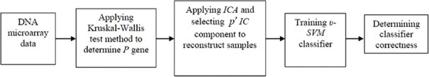
A microarray has thousands of spots, each of them consisting of different identified DNA strands, named probes. These spots are printed on glass slides by a robotic printer. Two types of microarray have the most application; microarrays based on complementary DNA (cDNA) and Oligonucleotide array which briefly named Oligo.[1] In cDNA array method, each gene is represented by a long strand (between 200 and 500 bps). cDNA is obtained from two different samples; test sample and reference one that are mixed in an array. Test and reference samples are denoted with red and green fluorescents, respectively (these two samples which have different wave lengths, are named Cy3 and Cy5).[3] If the two cDNA samples consist of trails that are a complement of a DNA probe, then the cDNA sample is mixed with spot. cDNA samples that are found their own complementary probe, are hybrid on array, and the remainder of samples are washed and then the array is scanned by a laser ray for determining the scaling of sample joined to spot. Hybrided microarray is scanned in red and green wavelength, and two images are obtained. Fluorescent intensity ratio in each spot demonstrates the DNA trail relative redundancy in two mixed cDNA samples on that spot. With surveying the gene expression levels ratio in two images, Cy3 and Cy5, gene expression study is done. Gene expression dimension can be the logarithm of the red to green intensity ratio.[4] Figure 1 shows the microarray data attaining steps.

Figure 1.

Different steps of obtaining microarray data

Microarray data is as a matrix with thousands of columns and hundreds of rows, each row and column representing a sample and gene, respectively. A gene expression level is related to the generated protein value. Gene expression provides a criterion for measuring the gene activity under the special biochemical situation. The gene expression is a dynamic process that can vary in transient or steady-state form. Thus, it can resound momentary and insolubility variations in the biologic state of cells, tissues and organisms.[5] Using the microarray technology, it is possible to analyze the pattern and gene expression level of different types of cells or tissues.

The main issue in microarray technology is the extra number of data obtained from a microarray that is merged to noisy data.[6] High dimensions of features and relatively low number of samples result in outbreak problems in microarray data analyzing. These problems are as follows:

• Increasing the computational cost and classifiers complexity

• Decreasing the ability of classifiers extension and reducing their validity to forecast the new samples

• Due to the high ratio of features to samples, it is highly possible that irrelevant genes represent themselves when finding genes with different expressions and making the forecasting models

• Explanation of genes causing disease is difficult. As a biological point of view, only a small set of genes are related to disease. Therefore, data related to the majority of genes actually have noisy background role, which can fade the effect of that small but important subset. Hence, concentration on smaller sets of gene expression data results in a better explanation of the role of informative genes.

There is also a major problem named “multicollinearity” in the data matrix with highly correlated features. If there is no linear relationship between the regressors, they are said to be orthogonal. Multicollinearity is a case of multiple regression in which the predictor variables are themselves highly correlated. If the goal is to understand how the various X variables impact Y, then multicollinearity is a big problem. Multicollinearity is a matter of degree, not a matter of presence or absence.[7]

The first important step to analyze the microarray data is reducing the noninformative genes or on the other hand, genes selection for the classification task. In general, three features (gene) selection models exist.[8] The first model is filter model that carries out the features selection and classification in two separated steps. This model selects the genes as effective genes, ^that have high discriminative ability. It is independent of classification or training algorithm and also is simple and fast. The second model is wrapper model that carries out the features selection and classification in one process. This model uses the classifier during the effective genes selecting process. In other words, the wrapper model uses the training algorithm to test the selected gene subset. The accuracy of wrapper model is more than filter one. Different methods are represented for selecting the appropriate subsets based on wrapper model in literatures. Evolutionary algorithms are used with K-neighborhood nearest classifier for this aim.[9] Parallel genetic algorithms are extended by applying adaptive operations[10] Also[11] genetic algorithm and support vector machine (SVM) hybrid model are used to select a set of genes. Gene selection and classification problem is discussed as a multi objective optimization problem[12] in which the number of features and misclassified samples are reduced, simultaneously.

Finally in hybrid models, selecting a set of effective genes is done during the training process by a particular classifier. A sample of this model is using a SVM with recursive feature elimination. The idea of this method is eliminating the genes one by one and surveying the effect of this elimination on the expected error.[13] Recursive feature elimination algorithm is a backward feature ranking method. In other words, a set of genes that is eliminated at the last step, attains the best classification results, while these genes may do not have good correlation with the classes. Hybrid models can be considered as an extended form of wrapper model. Two other samples of the hybrid model are mentioned in Saeys, et al.[14] and Goh, et al.[15]

In recent years, different statistical techniques have been presented to reduce gene expression level dimension in microarray data based on factor analysis methods. Liebermeister showed in Liebermeister[16] that each gene expression level can be expressed as a linear combination of independent components (ICs). Huang uses IC analysis in order to model gene expression data and then apply efficient algorithms to classify these data.[17] Using this method not only results in efficient usage of high order statistical information found in microarray data, but also makes it possible to use adjusted regression models in order to estimate correlated variables. In Kim, et al.[18] three different types of independent component analysis (ICA) are used to analyze gene expression data time series, which are: Selective independent component analysis (SICA), tICA, stICA.

Much of the information that perceptually distinguishes faces are contained in the higher order statistics of the microarray time series data. Since ICA gets more than second order statistics (covariance), it appears more appropriate with respect to principle component analysis (PCA). The technical reason is that second-order statistics corresponds to the amplitude spectrum of the signal (actually, the Fourier transforms of the autocorrelation function of the signal corresponds to its power spectrum, the square of the amplitude spectrum). The remaining information, high-order statistics, corresponds to the phase spectrum.

The basis of ICA method is to decompose multipath observed signals into independent statistical data (source signals).[19] However in practice, the number of source signals is indefinite, and it results in instability of ICA method. Because of that, a method called selective ICA method has been presented in this paper to resolve the instability problem. In this method, a set of independent components (ICs) that have a minor reconstruction error for reconstructing sample for classification is selected instead of extracting all source signals. Also, because limited number of samples is gained in practice, we propose a new class of support vector algorithms for classification named υ-SVM[20] as a cancer cells classifier. In this algorithm, a parameter υ lets one effectively control the number of support vectors. While this can be useful in its own right, the parameterization has the additional benefit of enabling us to eliminate one of the other free parameters of the algorithm: The accuracy parameter ε in the regression case and the regularization constant C in the classification case.

The rest of the paper is organized as follows; In Section II, the used microarray databases are introduced. In Section III, Kruskal–Wallis algorithm has been introduced for effective genes selection. ICA method and also efficient ICA algorithm for resolving its instability problem have been introduced in Section IV and V, respectively. In Section VI, modified υ-SVM algorithm is propounded. Block diagram of our proposed algorithm and implementation results based on three microarray datasets are presented in Section VII. Comparison of proposed algorithm and other existing methods is cited in Section 8, and finally conclusion is in Section VIII.

DATASETS USED IN THIS PAPER

In this paper, we have used three microarray databases that are described in this section. It must be noted that all samples are measured using Oligonucleotide arrays with high density.[21] The used data in this paper is extracted from reference.[22]

Leukemia

This database consists of 72 samples of microarray tests with 7129 gene expression levels. The main problem is discrimination of two types of leukemia cancer, acute lymphoblastic leukemia (ALL) and acute myeloid leukemia (AML). Data are divided to two groups; 34 control samples (20 cases are related to ALL and 14 cases are related to AML) used in the test process, and 38 cancer samples (27 cases are related to ALL and 11 cases are related to AML) used in the training process.

Breast Cancer

This database consists of 97 samples of microarray tests with 24481 gene expression levels. Data are divided to two groups; 19 control samples (12 cases are related to relapse samples and 7 cases are related to nonrelapse samples) used in the test process, and 78 cancer samples (34 cases are related to relapse samples and 44 cases are related to nonrelapse samples) used in the training process.

Lung cancer

This database consists of 181 samples of microarray tests with 12533 gene expression levels. Data are divided to two groups; 149 control samples (15 cases are related to malignant pleural mesothelioma (MPM) samples and 134 cases are related to adenocarcinoma (ADCA) samples) used in the test process, and 32 cancer samples (16 cases are related to MPM samples and 16 cases are related to ADCA samples) used in the training process.

USING KRUSKAL–WALLIS METHOD IN ORDER TO SELECT EFFECTIVE GENES

DNA microarray data experiments provide the possibility to record expression level of thousands of genes at the same time. But, only a small set of genes are appropriate for cancer recognition. Huge amount of data cause a growth in computational complexity and, as a result, classifying speed reduces.[23] Hence, selecting a useful set of genes before classifying is vital. In this paper, Kruskal–Wallis[24] test method has been used to select effective genes with noticeable oscillations in their expression level. The Kruskal–Wallis measure is a nonparametric method for testing whether samples originate from the same distribution. It is used for comparing more than two samples that are independent, or not related.

Assume data matrix X_int = (x_ij)_pint×n, with n to be the number of samples, p_int to be the number of prime genes and x_ij to be expression level of i^th gene in j^th sample. Furthermore, assume there is an independent class of samples in X_int, according to the number of k, as X_c ~ F(x - θ_c) and c = 1,2,…,k.

F distributions are continues functions, which are similar to each other, and θ_c parameter setting is different in them. Also, assume are samples of X_c. So, n can be displayed as , and order in X_int equals to R_cq. If we indicate summation and average of X_c with and respectively, the average amount of X_int will be 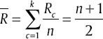. Kruskal–Wallis method uses 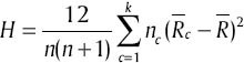to indicate gene expression variety among different classes.

INDEPENDENT COMPONENTS ANALYSIS METHOD

Independent component analysis is a method to process signal, based on high order statistical information. It decomposes multipath signals into independent statistical components, source signals. ICs expression reduces data noise. Considering selective genes P through Kruskal–Wallis test method, ICA can be modeled perceiving below assumptions:[16]

• Source signals are independent statistically

• The number of source signals is lower than or equal to the number of observed signals, and

• The number of source signals with Gaussian distribution is 0 or 1, and Gaussian combinational signals are inseparable

• Perceiving upper assumptions ICA model for X(t) is expressed as below:

X(t) = A*S(t)      (1)

Where X(t) = [X₁(t),X₂(t),···,X_p(t)]^T is a data matrix with p × n dimensions, and its rows correspond with observed signals and its columns correspond with the number of samples. A = [a₁,a₂,···,a_m] is combination matrix with p×m dimensions and S(t) = [S₁(t),S₂(t),···,S_m(t)]^T is source signal matrix with m × n dimensions as its rows are independent statistically. Variables found in S(t) rows are called ICs and X(t) observed signals form a linear combination with these ICs. ICs estimation is made with finding linear relation of observed signals. In other words, with estimating a W matrix, satisfying the equation below, this objective can be reached.

S(t) = A⁻¹ * X(t) = W * X(t)      (2)

There are different algorithms to perform ICA. In this paper, Fast-ICA (FICA) algorithm has been used to achieve IC components with equal variable number as the dimension of samples. Generally, when the number of source signals is equal to observation, reconstructed observed signals can contain comprehensive information.

SELECTIVE INDEPENDENT COMPONENTS ANALYSIS METHOD

In gene expression process, each IC component has a different biological importance and corresponds with a particular observed signal, which is described as a source signal of an expression gene. So, ICA contains useful information about gene expression. As the time series in gene expression process and in comparison with PCA algorithm, IC dominant components gained from ICA can be a describer of a greater structure of time series. Thus, analyzing selective components independently and selecting an accurate set of IC components to reconstruct new samples is a crucial issue. In Cheung and Xu[25] a method to eliminate the part of IC components, which make great construction error, has been presented. According to this method, in this paper, SICA method has been employed which we will explain in continue.

As cited in the previous section, by applying ICA, two combination matrixes A = [a₁,a₂,···,a_m] and S(t) = [S₁(t),S₂(t),···,S_m(t)]^T source signal are achieved. The i^th level of DNA microarray expression gene, is reconstructed by i^th IC of IC_i (i = 1,···,p); in other words, according to relation (1) we have:

Indeed, if gene expression level for i^th gene of main microarray is X_i∞, then error average square of reconstructed samples will be:

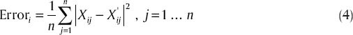
After calculating error average square amounts, we sort them into reconstructed samples, and select p′IC components with lower error. Presuming selected IC_i,a_i = a_i and S_i = S_i, otherwise a_i = 0 and S_i = 0. With this method, a new combination matrix A^ı and also a new source signal matrix S^ı is crated, and sample set X_new can be expressed as X_new = A^ı * S^ı based on ICs.

MODIFIED SUPPORT VECTOR MACHINE ALGORITHM

Support vector machine is a common method for classification work, estimation and regression. Its main concept is using separator hyper-plane to maximize the distance between two classes in order to design considered classifier. In a binary-SVM, training data is made of n sorted pair (x₁, y₁),···,(x_n, y_n), as:

y_i ∊ {-1,1} i,···,n      (5)

Thus, standard formula of SVM is as below:

And we have:

which in it ω ∊ R^m is a vector of training samples weights. Also, C is a constant parameter with a real amount and finally ζ is a slack variable. If ϕ(x_i) = x_i, relation (7) will show a linear hyper-plane with maximum distance. Also, relation (7) is a nonlinear SVM if ϕ can map x_i to a space with different number of dimensions of x_i space. The common method is to use relation (9):

And we have:

y^T α = 0,0 ≤ α_i ≤ C,i = 1,···,n      (9)

Where e is a vector of 1s, c is an upper bound, α_i is a multiplier variable of Lagrange kind, which its effect amount depends on C. Also, Q is a positively defined matrix, as Q_ij K(x_i,x_j) ≡ y_iy_jK(x_i,x_j) is a kernel function. It can be proved that, if α is selected for relation (9) efficiently, 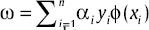will be efficient too. Training data is mapped to a space with different dimensions by ϕ function. In this case, the decision function is as below:

For a test vector like x, if:

Linear SVM classifies x in part 1. Also, when the problem is solved with relation,[9] vectors that for them α_i > 0 are set as support vectors. When we want to apply SVM to c classes instead of two classes, for each pair classes from the set of c classes, relation (9) becomes as below:

After solving optimizer phrase at relation (12), c(c-1)/2 decision functions are gained. To estimate the class label related to a vector like x, estimation process of all c(c-1)/2 classifiers has to be carried out and then a voting mechanism is applied to introduce the class that has been recognized by different classifiers most times, as label related to x.[26]

Main problem of SVM algorithm is constancy an uncontrollability of c parameter in relation (6). To resolve this problem, in this paper, υ-SVM algorithm has been used. This algorithm was introduced by Scholkopf in 2000.[27] In this algorithm, a pair of ω^Tx+ω₀ = ± ρ, ρ≥0 hyper-planes, and also a new parameter named υ∊(0,1) has been employed. With the use of this algorithm, relation (12) is modified as below:

And we have:

In Scholkopf and Smola[27] it has been proved that v is an upper bound on a part of training data and a lower bound on a part of support vectors. More details of this algorithm are in Theodoridis and Koutroumbas.[28]

GENERAL STRUCTURE OF PROPOSED ALGORITHM

The structure of modified SVM sub-classifier to classify DNA microarray data based on selective ICA is displayed in Figure 2. Performance details of this algorithm are as below.

Figure 2.

Modified support vector machine classifier structure in order to classify DNA microarray data based on ICA selective algorithm

Input

We indicate DNA microarray data with X_int and the number of genes that their expression level has lower oscillation among different classes with p, also, the number of ICs participating in reconstructing new samples with p, p^ı < p, and the number of υ-SVM sub-classifiers with N and υ-SVM sub-classifiers having most votes with N^ı.

Levels of Performing Algorithm

Applying Kruskal–Wallis test method to select P genes as their expression level has minor oscillation, and establishing sample set X.

For i = 1:N:

• Applying ICA on X in order to create combination matrix A and source signal matrix S

• Calculating reconstruction error of P IC according to Eq. (4)

• Selecting p′IC which their reconstruction error is roughly low for reconstructing new sample set, X_new

• Training υ-SVM sub-classifiers on X_new and using k-fold validation method to gain r_i correctness rate. The amount of k is considered to be 10.[29]

End.

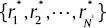
Correctness rate of all υ-SVM sub-classifiers are displayed as r = {r₁,r₂,···,r_N}; with selecting N^ı first sub-classifier which have a high accuracy, final rate of classifier accuracy r_i, can be achieved.

Output

correctness rates related to υ-SVM sub-classifiers with highest effect and correctness rate of υ-SVM sub-classifier.

All implementation levels of proposed algorithm have been carried out on a computer with 3.4 GHz processer and RAM memory of 1 GHz, also to apply υ-SVM algorithm, LIBSVM written in C⁺⁺ work environment. First, by applying Kruskal–Wallis test method on data related to blood, breast and lung cancers, we selected 10, 10 and 20 effective genes in these data, respectively, with the least oscillation of their expression level. Then, FICA algorithm was applied on selected genes to extract ICs. In the third step, appropriate ICs were selected according to their reconstruction error; as we selected 6, 7, 8 and 9 ICs from first data, and 16, 17, 18 and 19 from the second data, respectively. In forth step, we trained 25 υ-SVM sub-classifiers on reconstructed new sample. Finally, five υ-SVM sub-classifiers with roughly high correctness rate were selected using majority voting method. The success of majority voting depends on the number of members in the voting group. In this paper, we investigate the number of members in a majority voting group that gives the best results.

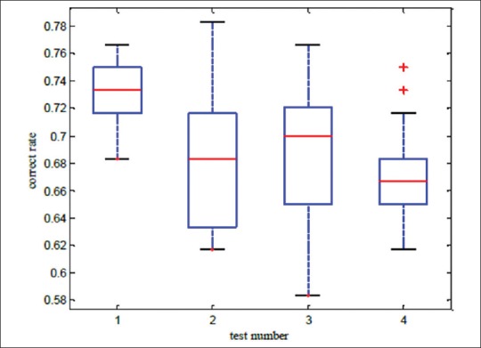
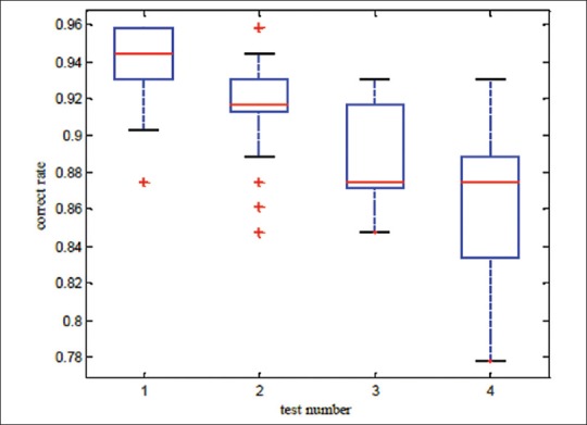
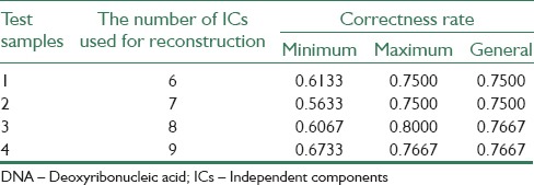
A lot of experimental results indicate that performing ICA process and selecting a set of ICs to reconstruct samples, makes correctness rate of υ-SVM sub-classifiers unstable. Thus, an appropriate number of sub-classifiers have to be trained to display all possible results. In this paper, four experiments have been carried out on 3 data bases. In Tables 1-3, minimum and maximum amounts of 25 υ-SVM sub-classifiers and also general correctness rate is demonstrated. Furthermore, Figures 2-4 demonstrate correctness rate box plot respectively in 4 experiments, as x and y axis are demonstrators of the number of test samples and correctness rate of the classifier, respectively. From Figures 3-5, it is observed that if a greater number of ICs are removed, five existing amounts in box-plots related to microarray data (minimum, first quadrature, medium, third quadrature, and maximum) will decline (except in the third experiment related to lung cancer). This subject shows that correctness rate of classifier changes according to the number of used ICs to reconstruct. If a greater number of ICs are removed, general correctness rate of the classifier proportioned to each sub-classifier will improve, apparently. Similar results can be achieved in Tables 1-3. As can be seen, correctness rate related to the whole classifier is more than correctness rate related to each classifier. For example, the ensemble correctness rate for 7 IC components in Leukemia dataset is 0.9444, while the maximum and minimum correctness rates for the same IC components in this dataset are 0.9306 and 0.8472, respectively. This point is worth noticing that in case of removing more ICs, classifier performance faces problem and becomes unstable. Thus, a trade-off must be established between the number of ICs used for reconstruction and correctness rate of the classifier.

Table 1.

Gained results with applying proposed algorithm on DNA microarray samples in leukemia cancer data base

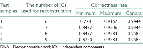
Table 3.

Gained results with applying proposed algorithm on DNA microarray samples in lung cancer data base

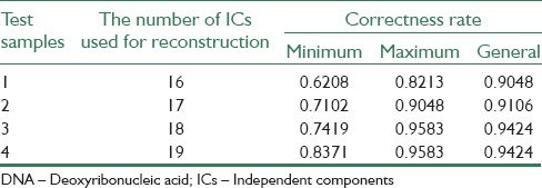
Figure 4.

Correctness rate box plot related to breast cancer

Figure 3.

Correctness rate box plot related to leukemia cancer

Figure 5.

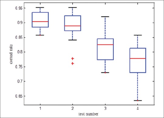
Correctness rate box plot related to lung cancer

Table 2.

Gained results with applying proposed algorithm on DNA microarray samples in breast cancer data base

RESULTS COMPARISON

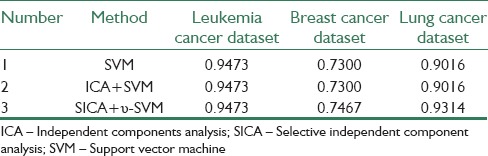
In order to display fidelity and capacity of suggested algorithm, SICA + υ-SVM, a comparison with other algorithms has been taken place, concerning highest correctness rates, which are demonstrated in Table 4. In the first method, microarray data has been classified directly with SVM method. In the second method, all ICA components have been employed to train SVM. As can be seen, the proposed algorithm yields the highest value of correctness rate in compare with other methods in two datasets (breast and lung cancer datasets). By way of illustration, our proposed algorithm exhibits relative improvements of 3.3% over ICA + SVM and SVM algorithms in Lung cancer dataset. Furthermore, it is obvious that if all ICs are used to reconstruct new samples, correctness rate of sub-classifier will not always be better than employing υ-SVM directly, while, with selecting an appropriate set of ICs, the result improves.

Table 4.

Comparing proposed algorithm with other existing methods concerning highest correctness rate

CONCLUSION

Cancer gene expression profiles are not normally-distributed, either on the complete-experiment or on the individual-gene level.[30] Instead, they exhibit complex, heavy-tailed distributions characterized by statistically-significant skewness and kurtosis. The non-Gaussian distribution of this data affects identification of differentially-expressed genes, functional annotation, and prospective molecular classification. These effects may be reduced in some circumstances, although not completely eliminated, by using nonparametric analytics.

In this paper, in order to resolve instability problem of ICs analysis algorithm, selective ICA algorithm has been used. In this algorithm, samples reconstruction error has been employed to select an independent set of algorithms used in time series analysis. Samples are reconstructed by a set of ICs, and modified SVM sub-classifiers are trained, simultaneously and eventually, best sub-classifier with the highest correctness rate is selected using majority voting method. Suggested algorithm has been applied on three samples of microarray data, and in each sample, correctness rate of 25 sub-classifiers and also general correctness rate are calculated and compared. Simulation results were illustrated that proposed algorithm leads to reduce the dimension of microarray data and the classification accuracy improves because of using υ-SVM classifier. Also the feasibility and validity of the proposed algorithm has been improved in compare with other existence methods shown in Table 4.

REFERENCES

- 1.Wee A, Liew C, Yah H, Yang M. Pattern recognition techniques for the emerging field of bioinformatics: A review. Pattern Recognit. 2005;38:2055–73. [Google Scholar]
- 2.Saberkari H, Shamsi M, Heravi H, Sedaaghi MH. A fast algorithm for exonic regions prediction in DNA sequences. J Med Signals Sens. 2013;3:139–49. [PMC free article] [PubMed] [Google Scholar]
- 3.Chu F, Wang L. Applications of support vector machines to cancer classification with microarray data. Int J Neural Syst. 2005;15:475–84. doi: 10.1142/S0129065705000396. [DOI] [PubMed] [Google Scholar]
- 4.Lu Y, Han J. Cancer classification using gene expression data. Inf Syst Data Manage Bioinform. 2003;28:243–68. [Google Scholar]
- 5.Brazma A, Vilo J. Gene expression data analysis. FEBS Lett. 2000;25(480):17–24. doi: 10.1016/s0014-5793(00)01772-5. [DOI] [PubMed] [Google Scholar]
- 6.Sehhati MR, Dehnavi AM, Rabbani H, Javanmard SH. Using protein interaction database and support vector machines to improve gene signatures for prediction of breast cancer recurrence. J Med Signals Sens. 2013;3:87–93. [PMC free article] [PubMed] [Google Scholar]
- 7.Chen Y, Zhao Y. A novel ensemble of classifiers for microarray data classification. Appl Soft Comput. 2008;8:1664–9. [Google Scholar]
- 8.Guyon I, Elisseeff A. An introduction to variable and feature selection. J Mach Learn Res. 2003;3:1157–82. [Google Scholar]
- 9.Li L, Weinberg CR, Darden TA, Pedersen LG. Gene selection for sample classification based on gene expression data: Study of sensitivity to choice of parameters of the GA/KNN method. Bioinformatics. 2001;17:1131–42. doi: 10.1093/bioinformatics/17.12.1131. [DOI] [PubMed] [Google Scholar]
- 10.Jourdan L. France: University of Lille; 2003. Metheuristics for knowledge discovery: Application to genetic data. Ph.D. [Google Scholar]
- 11.Peng S, Xu Q, Ling XB, Peng X, Du W, Chen L. Molecular classification of cancer types from microarray data using the combination of genetic algorithms and support vector machines. FEBS Lett. 2003;555:358–62. doi: 10.1016/s0014-5793(03)01275-4. [DOI] [PubMed] [Google Scholar]
- 12.Reddy AR, Deb K. Classification of two-class cancer data reliably using evolutionary algorithms. Technical Report, KanGAL. 2003 [Google Scholar]
- 13.Guyon I, Weston J, Barnhill S, Vapnik V. Gene selection for cancer classification using support vector machines. Mach Learn. 2002;46:389–422. [Google Scholar]
- 14.Saeys Y, Aeyels Degroeve S, Rouze D, Van de peer YP. Enhancement genetic feature selection through restricted search and Walsh analysis. IEEE Trans Syst Man Cybern Part C. 2004;34:398–406. [Google Scholar]
- 15.Goh L, Song Q, Kasabov N. A novel feature selection method to improve classification of gene expression data. Proceedings of 2nd Asia-Pacific Conference on Bioinformatics. 2004:161–6. [Google Scholar]
- 16.Liebermeister W. Linear modes of gene expression determined by independent component analysis. Bioinformatics. 2002;18:51–60. doi: 10.1093/bioinformatics/18.1.51. [DOI] [PubMed] [Google Scholar]
- 17.Huang DS, Zheng CH. Independent component analysis based penalized discriminate method for tumor classification using gene expression data. J Bioinform. 2006;22:1855–62. doi: 10.1093/bioinformatics/btl190. [DOI] [PubMed] [Google Scholar]
- 18.Kim SJ, Kim JK, Choi SJ. Independent arrays or independent time courses for gene expression time series data analysis. J Neurocomputing. 2008;71:2377–87. [Google Scholar]
- 19.Carpentier AS, Riva A, Tisseur P, Didier G, Hénaut A. The operons, a criterion to compare the reliability of transcriptome analysis tools: ICA is more reliable than ANOVA, PLS and PCA. Comput Biol Chem. 2004;28:3–10. doi: 10.1016/j.compbiolchem.2003.12.001. [DOI] [PubMed] [Google Scholar]
- 20.Mohamad MS, Deris S, Illias RM. A hybrid of genetic algorithm and support vector machine for features selection and classification of gene expression microarray. Int J Comput Intell Appl. 2005;5:91–107. [Google Scholar]
- 21.Ben-Dor A, Bruhn L, Friedman N, Nachman I, Schummer M, Yakhini Z. Tissue classification with gene expression profiles. J Comput Biol. 2000;7:559–83. doi: 10.1089/106652700750050943. [DOI] [PubMed] [Google Scholar]
- 22. [Last accessed on 2004 Jun 15]. Available from: http://www.datam.i2r.a-star.edu.sg/datasets/krb .
- 23.Shen Q, Shi WM, Kong W. New gene selection method for multiclass tumor classification by class centroid. J Biomed Inform. 2009;42:59–65. doi: 10.1016/j.jbi.2008.05.011. [DOI] [PubMed] [Google Scholar]
- 24.Ruxton G, Beauchamp G. Some suggestions about appropriate use of the Kruskal–Wallis test. J Anim Behav. 2008;76:1083–87. [Google Scholar]
- 25.Cheung YM, Xu L. An empirical method to select dominant independent components in ICA for time series analysis. Proceedings of the Joint Conference on Neural Networks. 1999:3883–7. [Google Scholar]
- 26.Settles M. Moscow, Idaho, U.S.A 83844: Department of Computer Sciences, University of Idaho; 2005. An Introduction to Particle Swarm Optimization. [Google Scholar]
- 27.Scholkopf B, Smola A, Williamson C, Bartlett PL. New support vector algorithms. Neural Comput. 2000;12:1207–45. doi: 10.1162/089976600300015565. [DOI] [PubMed] [Google Scholar]
- 28.Theodoridis S, Koutroumbas K. 4th ed. Elsevier Inc.: Academic Press; 2009. Pattern Recognition. [Google Scholar]
- 29.Dehnavi AM, Sehhati MR, Rabbani H. Hybrid method for prediction of metastasis in breast cancer patients using gene expression signals. J Med Signals Sens. 2013;3:79–86. [PMC free article] [PubMed] [Google Scholar]
- 30.Marko NF, Well RJ. Non-Gaussian distribution after identiication of expression pattern, functional annotation, and prospective classification in human cancer genomes. PloS One. 2012;7:1–15. doi: 10.1371/journal.pone.0046935. [DOI] [PMC free article] [PubMed] [Google Scholar]