

Abstract
Voxel-based morphometry from conventional T1-weighted images has proved effective to quantify Alzheimer's disease (AD) related brain atrophy and to enable fairly accurate automated classification of AD patients, mild cognitive impaired patients (MCI) and elderly controls. Little is known, however, about the classification power of volume-based morphometry, where features of interest consist of a few brain structure volumes (e.g. hippocampi, lobes, ventricles) as opposed to hundreds of thousands of voxel-wise gray matter concentrations. In this work, we experimentally evaluate two distinct volume-based morphometry algorithms (FreeSurfer and an in-house algorithm called MorphoBox) for automatic disease classification on a standardized data set from the Alzheimer's Disease Neuroimaging Initiative. Results indicate that both algorithms achieve classification accuracy comparable to the conventional whole-brain voxel-based morphometry pipeline using SPM for AD vs elderly controls and MCI vs controls, and higher accuracy for classification of AD vs MCI and early vs late AD converters, thereby demonstrating the potential of volume-based morphometry to assist diagnosis of mild cognitive impairment and Alzheimer's disease.
Keywords: Magnetic resonance imaging, Brain morphometry, Image segmentation, Alzheimer's disease, Mild cognitive impairment, Classification, Support vector machine
1. Introduction
Automated image-based brain morphometry analysis is increasingly used to quantify structural changes during normal aging and progression of certain diseases. This trend relates to both the widespread availability of brain imaging equipment in clinical routine and research, and the concurrent development of neuroinformatics which has materialized in several free as well as commercial image analysis software packages released over the past 15 years: SPM, FSL, FreeSurfer, BrainVisa, Mindboggle, NeuroQuant, and NeuroQLab, to mention a few.
Brain morphometry methods ultimately aim to extract imaging biomarker information that characterizes structural patterns of changes across groups of subjects, e.g. healthy and diseased. Methods vary in the type of imaging biomarkers they use. In voxel-based morphometry (VBM) from high resolution T1-weighted brain magnetic resonance imaging (MRI) data, imaging biomarkers are derived from processed images such as gray matter concentration maps, that are registered to a reference space in order to enable voxel-by-voxel comparisons across subjects (Ashburner and Friston, 2000). Several thousand voxel biomarkers need to be evaluated if the analysis is performed throughout the whole brain, as is common practice. Voxel-based brain morphometry has proven a valuable exploratory tool to characterize structural changes in various diseases as well as in several aspects of normal development (Mietchen and Gaser, 2009).
This paper focuses on the diagnosis of mild cognitive impairment (MCI) and Alzheimer's disease (AD). Several groups have shown that VBM combined with high-dimensional classification techniques can accurately distinguish AD patients, MCI patients and elderly controls (Liu et al., 2004; Klöppel et al., 2008; Duchesne et al., 2008; Cuingnet et al., 2011; Liu et al., 2012). Automatic voxel-based classification of AD patients vs frontotemporal demented patients has also been shown feasible (Klöppel et al., 2008; Davatzikos et al., 2008).
As a natural alternative and complementary approach to voxel-based morphometry, however, imaging biomarker information may also be obtained from volumes of specific brain structures of interest (Huppertz et al., 2010; Giorgio and De Stefano, 2013). There is now widespread agreement that medial temporal atrophy, in particular hippocampal atrophy, is a sensitive AD biomarker (Frisoni et al., 2009, 2010; Jack et al., 2011). Note that other biomarkers than voxels and volumes include cortical thickness measurements (Fischl and Dale, 2000; Jones et al., 2000), cortical folding patterns (Mangin et al., 2004), and longitudinal metrics of volume changes (Freeborough and Fox, 1997), not to mention potential disease biomarkers available from other modalities than T1-weighted imaging.
It is not yet clear how accurate fully automated volume-based morphometry (VolBM) can be at predicting disease compared to VBM. Cuingnet et al. (2011) reported hippocampus volume estimation methods that are competitive with whole-brain VBM to detect AD at an early stage. Other studies showed that volumes of medial temporal lobe regions computed using NeuroQuant exhibit statistically significant differences between early AD patients and controls (Brewer et al., 2008) and correlate with clinical scores (Kovacevic et al., 2009).
It is sometimes argued that whole-brain voxel-level information is ideal for classification in that it captures the whole pattern of disease-induced anatomical changes. In practice, however, high-dimensional classifiers suffer from the so-called curse of dimensionality, which inherently limits their accuracy unless trained from unrealistically large datasets. Moreover, high-dimensional classifiers tend to appear as “black boxes” to clinicians as opposed to rather simple volumetric measures of brain tissue or structure that are well known to be affected by age or disease. The interpretation of voxel-based classifiers in terms of spatial patterns of changes is an open methodological issue (Gaonkar and Davatzikos, 2012).
We here provide an experimental evaluation of VolBM for automated AD and MCI classification, with comparison to the whole-brain VBM approach using SPM previously reported, e.g., in Klöppel et al. (2008) and Cuingnet et al. (2011). The remainder of this paper is structured as follows. Sections 2–4 describe the data, brain morphometry algorithms and multivariate classification algorithms used in our evaluation. Experimental results are reported in Section 5 and discussed in Section 6.
2. Analysis dataset
2.1. ADNI background
Data used in the disease classification experiments described in the following were obtained from the Alzheimer's Disease Neuroimaging Initiative (ADNI) database (adni.loni.ucla.edu). The ADNI was launched in 2003 by the National Institute on Aging (NIA), the National Institute of Biomedical Imaging and Bioengineering (NIBIB), the Food and Drug Administration (FDA), private pharmaceutical companies and non-profit organizations, as a $60 million, 5-year public–private partnership. The primary goal of ADNI has been to test whether serial magnetic resonance imaging (MRI), positron emission tomography (PET), other biological markers, and clinical and neuropsychological assessment can be combined to measure the progression of mild cognitive impairment (MCI) and early Alzheimer's disease (AD). Determination of sensitive and specific markers of very early AD progression is intended to aid researchers and clinicians to develop new treatments and monitor their effectiveness, as well as lessen the time and cost of clinical trials. The Principal Investigator of this initiative is Michael W. Weiner, MD, VA Medical Center and University of California — San Francisco. ADNI is the result of the efforts of many co-investigators from a broad range of academic institutions and private corporations, and subjects have been recruited from over 50 sites across the U.S. and Canada. The initial goal of ADNI was to recruit 800 subjects but ADNI has been followed by ADNI-GO and ADNI-2. To date these three protocols have recruited over 1500 adults, ages 55 to 90, to participate in the research, consisting of cognitively normal older individuals, people with early or late MCI, and people with early AD. The follow-up duration of each group is specified in the protocols for ADNI-1, ADNI-2 and ADNI-GO. Subjects originally recruited for ADNI-1 and ADNI-GO had the option to be followed in ADNI-2. For up-to-date information, see www.adni-info.org.
2.2. ADNI standardized analysis set
Our analysis dataset was obtained from the ADNI standardized analysis sets described in Wyman et al. (2012), which consist of both 1.5 Tesla (1.5 T) and 3 Tesla (3 T) good quality T1-weighted MR images, from different acquisition systems and vendors, of individuals diagnosed as either normal, MCI, or AD based on careful clinical assessment. AD diagnosis is estimated to have an accuracy rate of about 90% using consensus criteria for probable AD (definite AD requires autopsy confirmation), and diagnostic accuracy is lower at pre-symptomatic stages. A fraction of subjects may therefore be misdiagnosed, for instance some pre-clinical AD subjects may be diagnosed normal or MCI, and some other subjects may be diagnosed AD while suffering from other dementias. It should therefore be kept in mind that the classification accuracy measures reported in Section 5 are inherently lowered by diagnosis uncertainty, assuming that automatic classification errors and diagnosis errors are weakly correlated, which is reasonable given that ADNI diagnosis was not based on morphometry.
We used the screening scans from the 1.5 T dataset (818 image sets corresponding to distinct subjects: 229 controls, 401 MCI, 188 AD) and the baseline scans from the 3 T dataset (151 image sets corresponding to distinct subjects: 47 healthy, 71 MCI, 33 AD). All subjects from the 3 T dataset are also included in the 1.5 T dataset, having been scanned at 3 T less than 4 months after their 1.5 T scan. The analysis dataset was constituted by taking the standardized ADNI 1.5 T dataset and replacing every 1.5 T scan by the corresponding subject 3 T scan when available, resulting in a set of images with mixed field strengths (about 80% 1.5 T and 20% 3 T) from all distinct subjects with the same size and diagnosis repartition as the 1.5 T dataset.
For a fair comparison between morphometry methods, the images input to the different morphometry methods were the images corrected for gradient distortion, B1 inhomogeneity and bias field as provided by ADNI. Hence image artifacts are expected to have a minimal effect on morphometry results. Note that each of the tested methods (FreeSurfer, MorphoBox, SPM, see Section 3) performed a further bias field correction.
We also conducted experiments on the pure 1.5 T dataset that yielded very similar results to those obtained from the combined 1.5 T/3 T dataset, and are thus not reported. The 3 T dataset alone appeared too small to serve as a basis for meaningful statistical comparisons between morphometry methods.
3. Brain morphometry methods
3.1. SPM
SPM (Statistical Parametric Mapping, www.fil.ion.ucl.ac.uk/spm) is a popular neuroimaging analysis software that implements a VBM pipeline thoroughly described at the theoretical level in Ashburner and Friston (2000, 2005), Ashburner (2007), and Ashburner and Friston (2009) and at the practical level in Ashburner (2010). In this work, we used SPM version 8, abbreviated SPM8. In brief, the pipeline first converts an incoming MR scan into several tissue probability maps, including a GM probability map, using a Bayesian image segmentation algorithm called New Segment. The GM probability map is then spatially smoothed and warped to a reference space to enable voxel-by-voxel comparisons of different subjects. This normalization step involves rescaling the smoothed GM probability values, considered as voxel-wise GM concentrations, by the Jacobian determinants of the deformations in order to compensate for spurious volume variations introduced by the warping. In addition, the reference space itself is iteratively optimized from the GM and WM probability maps of different subjects using the DARTEL algorithm (Ashburner, 2007).
3.2. FreeSurfer
FreeSurfer (surfer.nmr.mgh.harvard.edu) is today probably the most widely used software for VolBM. It implements a complex image processing pipeline described in Fischl et al. (2002), Fischl (2012) and the references therein, which segments an incoming scan in a large number of anatomical structures and subsequently computes corresponding volumes. In this work, we used FreeSurfer version 5.1.0 and were mainly interested in temporal GM, total GM, hippocampus and ventricular volumes output by FreeSurfer as potential imaging biomarkers of AD-related brain atrophy.
A current limitation of FreeSurfer is its computational complexity compared to SPM, which may restrict its use in clinical routine. On an up-to-date single-processor PC, the FreeSurfer pipeline typically takes several hours to run for a single scan while SPM takes minutes. Other highly accurate volume extraction methods such as multi-template segmentation methods (Klein et al., 2005) also require heavy computational load.
3.3. MorphoBox
We implemented a brain volumetry algorithm that combines simple and fast image analysis methods in order to perform VolBM in computation time comparable with SPM without hardware optimization. This algorithm called MorphoBox is freely available as a web application (http://brain-morpho.epfl.ch) and is detailed in Appendix A.
One key algorithmic difference with FreeSurfer that enables reduced computation time is that MorphoBox splits the segmentation of anatomical structures into two sequential steps: 1) labeling of total intracranial volume (TIV) voxels in brain tissue (CSF, GM, CSF) similarly to SPM's New Segment except that no atlas-based prior is used at this stage; and 2) brain structure segmentation by combining tissue maps obtained in step 1 with anatomical masks derived from a single-subject template via nonrigid registration. In FreeSurfer, both steps are collapsed into one step that directly infers structure-wise labels using a local image intensity model (Fischl et al., 2002). Also note that, contrary to FreeSurfer, both MorphoBox and SPM perform soft tissue labeling, i.e., assign voxels to tissue weights as opposed to single tissue labels, hence accounting for partial volume effects to some extent. Table 1 summarizes the main differences between the segmentation methods underlying SPM, FreeSurfer and MorphoBox, respectively.
Table 1.
Comparison of the segmentation algorithms underlying the morphometry methods evaluated in this work.
| Segmentation model | Atlas prior | Labeling | |
|---|---|---|---|
| SPM | Tissue-wise | Yes | Soft |
| FreeSurfer | Structure-wise | Yes | Hard |
| MorphoBox | Tissue-wisea | No | Soft |
MorphoBox segments brain structures in a post-processing step, see text.
4. Multivariate disease classification
Automatic classification techniques based on multiple biomarkers can help the clinician to test a specific binary hypothesis regarding a particular subject, e.g., is the subject MCI or AD? If the subject is MCI, will he/she or not convert to AD within a certain time? Consistently with previous work on classification in AD, we used support vector machines (SVMs) (Cortes and Vapnik, 1995) as implemented in LIBSVM (Chang and Lin, 2011) to respectively perform automatic classification of AD patients vs healthy controls, MCI patients vs healthy controls, AD vs MCI patients, and early vs late AD converters among MCI patients. The previous study of Abdulkadir et al. (2011) indicates that disease classifiers can safely be trained on ADNI images acquired with heterogeneous hardware settings. In each classification scenario, we compared classification performances from three distinct feature sets: normalized voxelwise GM concentrations computed via SPM and a set of a priori chosen volumes extracted using either FreeSurfer or MorphoBox.
4.1. Voxel-based classification
For the sake of comparison of VolBM methods with conventional VBM, we implemented an SPM8-based classification method similar to the one described in Klöppel et al. (2008) using a linear hard-margin SVM classifier. The GM tissue probability maps in native space were obtained from SPM8 New Segment (Ashburner and Friston, 2005) and subsequently normalized to the population template generated from all images in the standardized ADNI dataset using the iterative DARTEL approach (Ashburner, 2007), a procedure that took about three days on a standard PC. GM probability values in template space were modulated by the Jacobian determinant of the deformation field in order to compensate for local volume changes induced by spatial normalization (Ashburner and Friston, 2000). Voxels were then excluded if their modulated GM probability was less than 0.2 or if short of significance (p > 0.05) according to a two-sample t-test (Chaves et al., 2009). The remaining voxels, of the order of 300,000 in our experiments, were detrended for age as recommended by (Dukart et al., 2011) and fed into the SVM classifier.
4.2. Volume-based disease classification
The rationale for selecting brain structures for volume-based classification was their known involvement in AD-related brain atrophy at an early or moderately advanced stage of the disease (Frisoni et al., 2010). We chose a set of 10 features consisting of the following normalized brain or ventricular volumes: total GM, left and right temporal GM, left and right hippocampus, total CSF, and lateral, 3 and 4 ventricles. All MorphoBox and FreeSurfer volumes were normalized by FreeSurfer's or MorphoBox's TIV, respectively, and used to train multivariate SVM classifiers. For consistency with Cuingnet et al. (2011), and in order to investigate the benefit of multivariate classification, we also evaluated univariate classifiers based on the hippocampus volume only for both FreeSurfer and MorphoBox.
In the case of FreeSurfer, the TIV (called intracranial volume in the FreeSurfer 5.1.0 documentation), total GM, and hippocampus and ventricular volumes were read directly from the asegstats output file. As suggested on the FreeSurfer wiki (surfer.nmr.mgh.harvard.edu/fswiki/CorticalParcellation), left and right temporal GM volumes were computed by summing up several ROI volumes found in the lh.aparc.stats and rh.aparc.stats files, respectively. These are the ROIs labeled as superior temporal, middle temporal, inferior temporal, transverse temporal, banks of the superior temporal sulcus, fusiform, entorhinal, temporal pole and parahippocampal according to the Desikan–Killiany atlas (Desikan et al., 2006). Likewise, the total CSF was computed by summing up all ventricular volumes and adding the remaining CSF volume corresponding to voxels classified as extraventricular CSF. In order to correct relative volumes for aging effects, we applied the same linear detrending method as for VBM (Dukart et al., 2011) to each volume.
A specificity of volume-based classification is that the number of volume features is typically much smaller than the number of training scans, implying that the classification problem is not linearly separable. Therefore, the linear hard-margin SVM is not applicable and we instead resorted to linear soft-margin SVM classifiers using an adjustable cost parameter C.
4.3. Evaluation of classification performance
The discriminative power of the different SVM classifiers was estimated by leave-one-out cross-validation, a classical procedure that excludes one subject, trains the classifier with the remaining subjects and then checks whether the left-out subject is well classified or not. Numbers of true positives (TP), false positives (FP), true negatives (TN) and false negatives (FN) were counted by repeating this scheme for every subject. AD patients were considered to be positives in the classification of AD patients vs healthy controls as well as in the classification of AD patients vs MCI patients. MCI patients were considered positives in the classification of MCI patients vs healthy controls. Likewise, AD converters were considered positives in the classification of AD converters vs non-converters among MCI subjects.
The following performance measures are reported in Section 5:
-
•
Sensitivity (SEN), the proportion of correctly classified positives: SEN = TP ∕ (TP + FN).
-
•
Specificity (SPE), the proportion of correctly classified negatives: SPE = TN ∕ (TN + FP).
-
•
Balanced accuracy (BACC), the average of sensitivity and specificity: BACC = (SEN + SPE) ∕ 2.
-
•
Positive predictive value (PPV), the proportion of true positives in detected positives: PPV = TP ∕ (TP + FP).
-
•
Negative predictive value (NPV), similar to PPV for negatives: NPV = TN ∕ (TN + FN).
-
•
Likelihood ratio positive, LR+ = SEN ∕ (1 − SPE), the post-test positive odds corresponding to even pre-test odds given a positive test.
-
•
Likelihood ratio negative, LR− = (1 − SEN) ∕ SPE, the post-test positive odds corresponding to even pre-test odds given a negative test.
Also, following Cuingnet et al. (2011), McNemar's chi square test using the Yates correction was applied to assess differences in accuracy between classifiers as well as to test whether each classifier was equivalent to a random classifier.
5. Results
5.1. Processing
All images were processed by SPM8, FreeSurfer 5.1.0 and MorphoBox. Both SPM and MorphoBox SPM terminated successfully in all cases while FreeSurfer failed to process 12 images for reasons that we did not further investigate. These cases, which are specified by their unique ADNI identifier in Appendix C, relate specifically to 2/229 controls, 2/401 MCI patients, 1/188 AD patient in the 1.5 T dataset, and 1/47 control, 4/71 MCI patients, 2/33 AD patient in the 3 T dataset. The FreeSurfer performance measures reported below are restricted to the standardized ADNI dataset excluding those cases. For the McNemar tests in multivariate classification, the images that could not be processed by FreeSurfer were counted as random classifications. The average computation time per image on a single-threaded 3 GHz processor with 8 GB RAM was about 8 min for MorphoBox, 10 h for FreeSurfer, and 5 min 30 s for SPM.
5.2. FreeSurfer/MorphoBox biomarker comparison
This section presents an experimental comparison between the two above described VolBM methods, FreeSurfer and MorphoBox. Direct evaluation of segmentation accuracy is impossible without knowledge of a ground truth. However, given two cohorts, one of normal subjects and one of patients (in this case, reliably diagnosed MCI or AD subjects), we may assess the ability of the respective methods to detect diseased subjects using a particular brain structure volume.
To that end, we defined for each structure of interest an age-matched normative range for volumes normalized by the TIV according to the method under consideration. This was done using linear regression against age on the healthy cohort, as depicted in Figs. 1–3. More specifically, normative ranges were defined as the linear regression prediction intervals corresponding to a given percentile under the simplifying assumption that normalized volumes are normally distributed at each age with constant variance. Note that normative ranges obtained under more realistic regression models, e.g. log-normal or nonlinear (Walhovd et al., 2011), turned out to have little impact on this analysis. We used one-sided intervals of the form (c,+∞) to detect atrophied structures and (−∞,c) to detect hypertrophied structures. The higher the percentile, the wider the range.
Fig. 1.

Linear regression plots for total GM volume estimation on the standardized ADNI dataset using FreeSurfer (left) and MorphoBox (right). Black and red dots represent healthy controls and AD patients, respectively. Dotted lines represent the 10 and 90 percentiles for the controls.
Fig. 2.

Linear regression plots for temporal GM volume estimation using FreeSurfer (left) and MorphoBox (right). Black and red dots represent healthy controls and AD patients, respectively. Dotted lines represent the 10 and 90 percentiles for the controls.
Fig. 3.

Linear regression plots for hippocampus volume detection on the standardized ADNI dataset using FreeSurfer (left) and MorphoBox (right). Black and red dots represent healthy controls and AD patients, respectively. Dotted lines represent the 10 and 90 percentiles for the controls.
Receiver operating characteristic (ROC) curves shown in Fig. 4 express the proportion of diseased subjects found outside the normative range (sensitivity) as a function of the proportion of normal subjects outside the normative range (1–specificity) for several volumetric biomarkers. Abnormality detection rates, defined for a biomarker as the value on the corresponding ROC curve where sensitivity equals specificity, were evaluated in both the AD and MCI cohorts for several imaging biomarkers relevant to Alzheimer's disease (Frisoni et al., 2010) and compared between FreeSurfer and MorphoBox, see Table 2. For consistency, FreeSurfer and MorphoBox volumes were normalized by their respective own total intra-cranial volume (TIV) estimates.
Fig. 4.

ROC curves corresponding to Figs. 1–3 for AD detection on the standardized ADNI dataset using, from left to right: total GM, temporal GM, and hippocampus normalized volumes estimated by FreeSurfer and MorphoBox, respectively.
Table 2.
Single-biomarker abnormality detection rates for FreeSurfer and MorphoBox.
| Biomarker | AD |
MCI |
||
|---|---|---|---|---|
| FreeSurfer | MorphoBox | FreeSurfer | MorphoBox | |
| Left hippocampus | 82% | 77% | 70% | 66% |
| Right hippocampus | 79% | 76% | 70% | 67% |
| Hippocampus | 83% | 78% | 71% | 69% |
| Left temporal GM | 77% | 80% | 65% | 67% |
| Right temporal GM | 75% | 79% | 64% | 65% |
| Temporal GM | 78% | 81% | 66% | 67% |
| Cortical GM | 70% | 73% | 63% | 64% |
| Total GM | 71% | 72% | 64% | 64% |
| Total CSF | 64% | 72% | 56% | 63% |
Overall, abnormality detection rates obtained using MorphoBox and FreeSurfer turned out remarkably consistent on standardized ADNI data despite the different degrees of sophistication and computation time of the respective methods. FreeSurfer achieved higher accuracy than MorphoBox with its hippocampus volume measures but yielded slightly lower accuracy with GM measures. Both methods could detect about 80% AD patients and close to 70% MCI patients with equal specificity (true negative rate) with temporal lobe and hippocampus volume measures. Abnormality detection rates obtained with more global biomarkers were lower: about 70% AD patients and 65% MCI patients for cortical GM and total GM, and similarly for total CSF using MorphoBox (lower abnormality detection rates were found with total CSF using FreeSurfer, most likely because the FreeSurfer measure excludes most of the extraventricular CSF and may thus lack power in detecting CSF expansion).
Differences in abnormality detection rates reflect algorithmic differences between MorphoBox and FreeSurfer that unavoidably lead to different volume estimates. The soft labeling approach used in MorphoBox (see Appendix A) might better account for partial voluming at the GM/CSF and GM/WM interfaces, leading to possibly more discriminative global GM volume measures. On the other hand, the FreeSurfer hippocampus segmentation method, which uses local, as opposed to global, intensity distribution modeling (Fischl et al., 2002) could be better suited for the segmentation of small mixed gray/white structures such as the hippocampus. These findings are consistent with the observation from the plots in Figs. 1–3 that FreeSurfer hippocampus volumes appear strongly correlated with age than their MorphoBox counterparts, while the converse can be seen for total and temporal GM volumes.
5.3. Multivariate classification results
Tables 3–7 report classification results from SVMs independently trained with volumetric features from MorphoBox and FreeSurfer and whole-brain voxel-wise GM concentrations from SPM. As discussed in Subsection 4.1, volume-based and voxel-based feature sets have very different dimensions, respectively 10 for MorphoBox and FreeSurfer, and about 300,000 for SPM. As discussed in Section 4, a hard-margin SVM was used for SPM-based classifiers whereas soft-margin SVMs were used for both MorphoBox and FreeSurfer due to lack of linear separability. The reported VolBM classification results correspond to the SVM margin cost parameters that yielded the largest BACC among predefined values on an exponential grid C = 10− 3,…,103.
Table 3.
Binary multivariate classification results for AD vs normal.
| Method | Performance |
McNemar tests |
||||||||
|---|---|---|---|---|---|---|---|---|---|---|
| SEN | SPEC | BACC | PPV | NPV | LR+ | LR− | FreeSurfer | MorphoBox | SPM | |
| FreeSurfer | 82% | 88% | 85% | 84% | 86% | 6.83 | 0.20 | – | p < 0.0001 | p = 0.0736 |
| MorphoBox | 86% | 91% | 89% | 88% | 89% | 9.56 | 0.15 | p < 0.0001 | – | p = 1.0 |
| SPM | 82% | 94% | 88% | 92% | 86% | 13.67 | 0.19 | p = 0.0736 | p = 1.0 | – |
Table 4.
Binary multivariate classification results for MCI vs normal.
| Method | Performance |
McNemar tests |
||||||||
|---|---|---|---|---|---|---|---|---|---|---|
| SEN | SPEC | BACC | PPV | NPV | LR+ | LR− | FreeSurfer | MorphoBox | SPM | |
| FreeSurfer | 66% | 80% | 73% | 85% | 57% | 3.30 | 0.42 | – | p < 0.0001 | p < 0.0001 |
| MorphoBox | 69% | 83% | 76% | 88% | 61% | 4.06 | 0.37 | p < 0.0001 | – | p < 0.0001 |
| SPM | 78% | 68% | 73% | 81% | 63% | 2.44 | 0.32 | p < 0.0001 | p < 0.0001 | – |
Table 5.
Binary multivariate classification results for AD vs MCI.
| Method | Performance |
McNemar tests |
||||||||
|---|---|---|---|---|---|---|---|---|---|---|
| SEN | SPEC | BACC | PPV | NPV | LR+ | LR− | FreeSurfer | MorphoBox | SPM | |
| FreeSurfer | 69% | 64% | 67% | 47% | 81% | 1.92 | 0.48 | – | p = 0.2482 | p < 0.0001 |
| MorphoBox | 69% | 67% | 68% | 49% | 82% | 2.09 | 0.46 | p = 0.2482 | – | p < 0.0001 |
| SPM | 45% | 69% | 57% | 40% | 73% | 1.45 | 0.80 | p < 0.0001 | p < 0.0001 | – |
Table 6.
Binary multivariate classification results for AD converters vs non-converters within 3 years.
| Method | Performance |
McNemar tests |
||||||||
|---|---|---|---|---|---|---|---|---|---|---|
| SEN | SPEC | BACC | PPV | NPV | LR+ | LR− | FreeSurfer | MorphoBox | SPM | |
| FreeSurfer | 75% | 66% | 71% | 75% | 66% | 2.21 | 0.38 | – | p = 0.0133 | p < 0.0001 |
| MorphoBox | 64% | 71% | 68% | 75% | 60% | 2.21 | 0.51 | p = 0.0133 | – | p = 0.0003 |
| SPM | 66% | 54% | 60% | 66% | 54% | 1.43 | 0.63 | p < 0.0001 | p = 0.0003 | – |
Table 7.
Binary multivariate classification results for AD converters vs non-converters within 2 years.
| Method | Performance |
McNemar tests |
||||||||
|---|---|---|---|---|---|---|---|---|---|---|
| SEN | SPEC | BACC | PPV | NPV | LR+ | LR− | FreeSurfer | MorphoBox | SPM | |
| FreeSurfer | 71% | 65% | 68% | 63% | 72% | 2.03 | 0.45 | – | p = 0.04123 | p = 0.0005 |
| MorphoBox | 67% | 71% | 69% | 66% | 71% | 2.31 | 0.47 | p = 0.04123 | – | p < 0.0001 |
| SPM | 57% | 65% | 61% | 59% | 63% | 1.63 | 0.66 | p = 0.0005 | p < 0.0001 | – |
All evaluated morphometry methods tended towards higher classification performance, as measured for instance by the balanced accuracy (BACC), for AD vs normal classification (BACC ≥ 85%), than MCI vs normal (BACC ≅ 75%), AD vs MCI (BACC ≤ 70%) and early vs late AD conversion (BACC ≤ 70%), reflecting the increasing inherent difficulties of the respective classification problems. Nevertheless, all classifiers performed significantly above chance in all cases with the McNemar tests significant at p = 0.0001.
5.4. AD vs normal
In the AD vs normal classification, the MorphoBox-based and whole-brain SPM-based classifiers both reached almost 90% BACC, which is of the order of the AD diagnosis accuracy, and no classifier was found significantly more accurate than the other according to the McNemar test. As shown by the likelihood ratios LR+ and LR−, the SPM-based classifier turned out better at confirming AD suspicion, but poorer at confirming normality. FreeSurfer achieved a slightly smaller BACC of 85%, which is perhaps surprising but consistent with our previous experimental observation that some MorphoBox volumetric biomarkers achieved individually higher abnormality detection rate for AD subjects (see Subsection 5.2).
5.5. MCI vs normal
As expected, all methods proved less accurate for the classification of MCI vs normal than for AD vs normal, with BACC in the range 73–76%. Again, differences between classifiers were small, although statistically significant. The MorphoBox-based classifier turned out the most accurate to confirm MCI suspicion (LR+ = 4.06), but the SPM-based classifier was the most accurate to confirm normality (LR− = 0.32). The FreeSurfer-based classifier achieved a larger LR+ than SPM.
5.6. AD vs MCI
Differences between volume-based and voxel-based classifiers were found to be more significant for AD vs MCI than for AD vs normal and MCI vs normal. The drop in classification accuracy compared to AD vs normal and MCI vs normal was remarkably more pronounced for the SPM-based classifier, resulting in a relatively poor 57% BACC compared to 67–68% for FreeSurfer and MorphoBox, respectively. This suggests that distributions of voxel-wise GM concentrations might be too similar in AD and MCI populations for an optimal classification to be achieved using the implemented feature selection strategy (see Subsection 4.2), which ignores prior spatial information about AD atrophy.
5.7. Early vs late AD conversion
Among the MCI subjects present in the analysis dataset, we know from subsequent visits that some were later diagnosed AD in the course of the ADNI study. Specifically, 36 out of 401 MCI subjects are known to have converted to AD within one year while 157 did not; 111 converted within 2 years and 130 did not; 137 converted within 3 years and 103 did not. We may thus try to automatically classify AD converters vs non-converters depending on a given conversion time window using the same techniques as described above. In the following, we report classification experiments for time windows of 2 years and 3 years, given that a one-year time window does not provide a sufficient number of converters for statistically meaningful comparisons.
The results, reported in Tables 6 and 7, show classification accuracy levels quite similar to the AD vs MCI classification. Again, volume-based classification performed more accurately than whole-brain voxel-based classification. For a 2-year conversion threshold, FreeSurfer and MorphoBox provided similar results with 68% and 69% BACC, respectively, and similar likelihood ratios. For a 3-year conversion threshold, however, FreeSurfer turned out somewhat more accurate than MorphoBox, as shown by 71% BACC against 68% with the same LR+ 2.21 but lower LR− 0.38 against 0.51. The hippocampus volume might be the driving feature for classification when comparing two groups both affected by early-stage AD atrophy. Therefore, this outcome is in line with our previous observation (see Subsection 5.2) that FreeSurfer's hippocampus estimate tends to be more sensitive to disease than MorphoBox's.
5.8. Comparison with univariate classification
In order to assess the actual benefit of multivariate classification in VolBM approaches, we report in the Appendix (see Tables B.8–B.12) classification results obtained using FreeSurfer-based and MorphoBox-based SVM classifiers trained with the hippocampus volume only (univariate classification), as opposed to the above described 10 volume features (multivariate classification). As expected, univariate classifiers achieved smaller BACC values than multivariate classifiers in all classification scenarios, yet by smaller amounts for FreeSurfer (1–3%) than for MorphoBox (6–9%). FreeSurfer-based univariate classifiers actually performed very similarly to multivariate classifiers for early vs late AD converters, hence confirming the hippocampus preponderance in such classification tasks. The fact that univariate classification was clearly less accurate than multivariate classification for MorphoBox suggests that the relatively poorer hippocampus segmentation quality compared to FreeSurfer was compensated for by temporal lobe GM as well as possibly other GM and CSF measures.
6. Discussion
The goal of this study was to investigate the potential of VolBM to detect AD-related brain atrophy compared with conventional whole-brain VBM as implemented using SPM. We used both FreeSurfer and a simpler/faster in-house method called MorphoBox to benchmark VolBM methods against automatic binary disease classification, following a number of previous VBM studies in AD (Liu et al., 2004; Klöppel et al., 2008; Duchesne et al., 2008; Cuingnet et al., 2011; Liu et al., 2012). We trained SVM classifiers from a set of ten a priori chosen volumetric biomarkers known to be affected by AD at an early stage (Frisoni et al., 2010): left and right hippocampi, left and right temporal GM, lateral, 3 and 4 ventricles, total GM, and total CSF. SVMs trained respectively from FreeSurfer and MorphoBox were compared with SVMs trained from SPM-based GM concentration maps. Classification accuracy was evaluated on a standardized ADNI dataset comprising 818 1.5 T and 3 T scans from different subjects (229 controls, 401 MCI, 188 AD) using leave-one-out cross-validation.
VolBM yielded classification performance comparable, or superior, to whole-brain VBM in all tested classification scenarios. Specifically, VolBM using MorphoBox proved roughly equivalent to VBM for both AD vs normal and MCI vs normal classifications, and clearly more accurate for both AD vs MCI and early vs late AD converter classifications. A similar trend was observed for VolBM using FreeSurfer, although it turned out slightly less accurate than the SPM-based classification for AD vs normal.
FreeSurfer and MorphoBox yielded remarkably consistent results across classification experiments. The FreeSurfer-based classifier was found to be marginally less accurate than the MorphoBox-based one for AD vs normal, MCI vs normal and AD vs MCI, but slightly more accurate to classify converters vs non-converters within 3 years. Also, univariate SVMs trained with FreeSurfer hippocampus volumes only performed similarly to their multivariate versions, confirming the importance of hippocampal atrophy in early AD as well as the diagnostic value of highly accurate hippocampus segmentation methods.
Moderate differences in classification accuracy between FreeSurfer and MorphoBox reflect algorithmic differences that lead to different brain volume estimates in practice. Differences were evaluated using a single-biomarker abnormality detection approach, and did not give a clear cut advantage to either one or the other method. Global biomarkers such as total GM, temporal GM and total CSF volumes output by MorphoBox tended to be more sensitive to disease than their FreeSurfer counterparts, while there were strong indications that FreeSurfer's hippocampus volume estimates were more sensitive than MorphoBox's. Consequently, it is not surprising that FreeSurfer achieved relatively more accurate classification as morphometric differences between the groups under comparison were mainly localized in the hippocampal region as opposed to being widespread throughout the brain.
Our findings are in line with the observation of Cuingnet et al. (2011) that univariate SVMs using the hippocampus volume only are comparable to VBM for classification of controls vs MCI patients believed to convert to AD within 18 months. We here tested the possibility to enhance the discriminative power of volume-based classifiers through a multivariate feature set including other biomarkers than the hippocampus volume. Our results indicate that higher-scale biomarkers such as temporal GM, total GM or total CSF volumes play a beneficial role in disease classification, but the advantage of including such features was less clear for FreeSurfer than for MorphoBox.
We evaluated the whole-brain SPM-based morphometry classification approach reported to perform best by Cuingnet et al. (2011) in the AD vs normal classification among over twenty method variants, and the experimentally observed accuracy levels are consistent with previous studies that used the same implementation (Klöppel et al., 2008; Cuingnet et al., 2011). We speculate that the relatively poor performance of SPM-based classifiers in both AD vs MCI and early vs late AD converter classifications may be due to suboptimal voxel selection. Feature selection schemes that make use of prior spatial information about AD atrophy, e.g. by focusing on temporal regions, might prove more effective in such classification tasks involving localized statistical differences between the populations to be compared. The extent to which the SPM-based classification may be improved is however an area of open research and was out of the scope of this work.
7. Conclusion
Our results provide evidence that VolBM is a valuable alternative to whole-brain VBM to assist the diagnosis of Alzheimer's disease and mild cognitive impairment. Within the tested conditions, multivariate volume-based classification approaches overall performed better than SPM. Moreover, a conceptual advantage of VolBM for image-guided diagnosis is the ability to squeeze anatomical information into a few descriptors, thereby not only providing easily interpretable second-opinion information to the clinician, but also working around the difficult problem of high-dimensional feature selection for automated classification. In the future, it will be interesting to evaluate whether our findings extend to other neurological disorders than AD and MCI.
It was also shown that a simple and fast VolBM method, MorphoBox, yielded classification performance quite similar to the more sophisticated FreeSurfer method, suggesting that high segmentation accuracy may have limited impact on automated disease prediction and presumably low impact on final diagnosis. On the other hand, the availability of fast VolBM software that can be easily integrated into clinical workflows opens the way to a more extensive use of automated brain morphometry in clinical practice.
Acknowledgments
This work was partly supported by the CIBM of the UNIL, UNIGE, EPFL, HUG and CHUV and the Louis-Jeantet Foundation and Leenaards Foundation. The authors would like to thank Stefan Huwer for developing the image visualization tool used in Fig. A.6, David Romascano for his support on the implementation of the SPM-DARTEL pipeline, and Irina Radu for the advice and reviewing of the manuscript.
Fig. A.6.
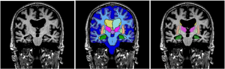
Example segmentation using MorphoBox: coronal view of an input MPRAGE volume and two distinct overlays of maximum probability tissue labels (CSF, GM, WM) and brain structures (lateral ventricles, central nuclei, hippocampus).
Data collection and sharing for this project was funded by the Alzheimer's Disease Neuroimaging Initiative (ADNI) (National Institutes of Health Grant U01 AG024904). ADNI is funded by the National Institute on Aging, the National Institute of Biomedical Imaging and Bioengineering, and through generous contributions from the following: Alzheimer's Association; Alzheimer's Drug Discovery Foundation; BioClinica, Inc.; Biogen Idec Inc.; Bristol-Myers Squibb Company; Eisai Inc.; Elan Pharmaceuticals, Inc.; Eli Lilly and Company; F. Hoffmann-La Roche Ltd. and its affiliated company Genentech, Inc.; GE Healthcare; Innogenetics, N.V.; IXICO Ltd.; Janssen Alzheimer Immunotherapy Research & Development, LLC.; Johnson & Johnson Pharmaceutical Research & Development LLC.; Medpace, Inc.; Merck & Co., Inc.; Meso Scale Diagnostics, LLC.; NeuroRx Research; Novartis Pharmaceuticals Corporation; Pfizer Inc.; Piramal Imaging; Servier; Synarc Inc.; and Takeda Pharmaceutical Company. The Canadian Institutes of Health Research is providing funds to support ADNI clinical sites in Canada. Private sector contributions are Rev November 7, 2012 facilitated by the Foundation for the National Institutes of Health (www.fnih.org). The grantee organization is the Northern California Institute for Research and Education, and the study is coordinated by the Alzheimer's Disease Cooperative Study at the University of California, San Diego. ADNI data are disseminated by the Laboratory for Neuro Imaging at the University of California, Los Angeles. This research was also supported by NIH grants P30 AG010129 and K01 AG030514.
Ahmed Abdulkadir and Stefan Klöppel were funded by a grant by the Deutsche Forschungsgesellschaft (KL2415/2-1) to Stefan Klöppel.
Appendix A. MorphoBox algorithm description
Appendix A.1. Manual template construction
A T1-weighted MR scan of a 64 year-old female with no alcohol dependence and no known central nervous system disorder was subjectively chosen as a template image to help automated image segmentation. The scan was acquired on a 3 Tesla scanner 32-head channel coil (Magnetom Trio a Tim system, Siemens Healthcare, Erlangen, Germany) at Lausanne University Hospital, Switzerland, using the ADNI-2 MPRAGE protocol with a 2-fold acceleration (Jack et al., 2010), yielding 256 × 240 × 160 voxels with slightly anisotropic size 1 × 1 × 1.2 mm3. Various anatomical structures were drawn by a neurologist on the template image and corrected by two neuroradiologists on consent. These include: the total intracranial volume (TIV) defined by the hemispheric and cerebellar gray matter (GM), white matter (WM) and the intracranial cerebrospinal fluid (CSF); lateral, third and fourth ventricles; cerebellum; thalamus; putamen; pallidum; caudate nucleus; and hippocampus. Every bilateral structure was split into two distinct masks. The cortex was also parcellated in ten regions corresponding to the frontal, temporal, parietal, and occipital lobes and the cerebellum in both hemispheres.
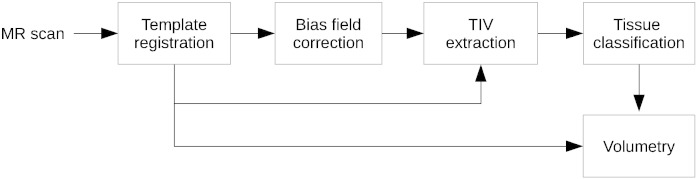
Appendix A.2. Image processing pipeline
The volume extraction algorithm is sketched in Fig. A.5. It takes as input an MPRAGE volume previously corrected for B1 receive (Narayana et al., 1988) and gradient distortion (Schmitt, 1985). A related important aspect that we do not discuss here is the quality control and artifact correction. Whereas ADNI takes care of this aspect for the standardized dataset, we employ in our clinical settings automated image quality assessment (Mortamet et al., 2009), artifact corrections and checkup for acquisition parameter compliance on the scanner console.
Fig. A.5.
Sketch of the MorphoBox processing pipeline.
Appendix A.2.1. Template-to-subject registration
The template image is non-rigidly registered onto the input MR image via a spatial transformation from the input image space to the template image space under the form:
where A is a 9-parameter affine transformation (translation and rotation followed by anisotropic scaling) and D is a free-form diffeomorphic displacement field. Registration proceeds by first estimating A by maximizing normalized mutual information (Studholme et al., 1998) using a gradient ascent algorithm, and resampling the template image accordingly. The displacement field D is then estimated using a fast iterative scheme that maximizes the local correlation between the input image and the affine-transformed template image by successive compositions of smooth incremental displacements (Chefd'hotel et al., 2002).
Appendix A.2.2. Bias field correction
Following registration, the input image is corrected for bias field using an expectation–maximization (EM) algorithm similar to Ashburner and Friston (2005). This uses a simple 4-class Gaussian mixture intensity model representing GM, WM, CSF and non-brain tissue, and is constrained by template-based tissue prior probability maps resampled to the input image space from the transformation T estimated in the registration step. Such priors were computed using the DARTEL tool of SPM8 (Ashburner and Friston, 2009) from a dataset of 136 MR scans of healthy subjects (41 ± 25 years) acquired at Lausanne University Hospital, Switzerland, in the same conditions as the template image. The correction field (inverse bias field) is modeled as a 3-degree spatial polynomial. To speed up computation, the M-step objective is approximated using a second-order Taylor expansion, resulting in efficient linear updates for the correction field coefficients.
Appendix A.2.3. Skull stripping
Next, the TIV template mask is resampled to the input image space according to the composed transformation T, which provides a reasonably accurate skull stripping where errors (due to included meninges and cut brain tissues) usually represent up to 1% of the TIV as assessed by visual inspection.
Appendix A.2.4. Brain tissue classification
The TIV restricted image is then submitted to a completely template-free tissue classification algorithm in order to avoid bias in tissue labeling towards the particular cohort involved in a probabilistic template construction (Ribes et al., 2011). At this stage, the image appearance model is a 5-class Gaussian mixture, which better accounts for intensity variations within CSF and GM (e.g., due to partial voluming) than a simple 3-class model, as discussed for instance by Bach Cuadra et al. (2005). The classes roughly represent ventricular CSF, sulcal CSF, cortical GM, deep GM and WM. Tissue classification is made robust to noise by incorporating a stationary Markov–Potts prior model (Van Leemput et al., 1999; Bach Cuadra et al., 2005) with a 6-neighborhood system. Practical model fitting is carried out using a variational expectation–maximization (VEM) algorithm, which is numerically more stable than other schemes commonly used in brain image analysis (Roche et al., 2011).
The VEM algorithm requires accurate initial guesses of the mean tissue intensities to work robustly. An initialization method that we found effective is to detect the three zero-crossings of the smoothed histogram first derivative, and consider them as the initial mean intensities corresponding respectively to ventricular CSF, cortical GM and WM. The additional two classes (mainly representing sulcal CSF and deep GM but also voxel intensities affected by partial voluming) are initialized by averaging adjacent values. We tested other initialization methods that make use of the 3-class mixture model fit performed in the bias field correction step, which however proved less effective for disease prediction. The VEM algorithm outputs five posterior probability maps, which are converted into three maps corresponding to CSF/GM/WM by simply adding the ventricular and sulcal CSF maps, on the one hand, and the cortical and deep GM maps, on the other hand.
Appendix A.2.5. Volumetry
Finally, the tissue probability maps are combined with the masks resampled from the template via transformation T computed in the template-to-subject registration step to produce regional volume estimates. Lobe-wise GM volumes are computed by summing up GM probabilities over the template-based parcels. The same approach is used with CSF probabilities to compute ventricular volumes. Hippocampus, central nuclei and cerebellum volumes are computed by summing up GM and WM probabilities over the relevant masks.
Appendix B. Classifiers using hippocampus volume only
Table B.8.
Binary univariate classification results for AD vs normal.
| Method | Performance |
McNemar tests |
|||||||
|---|---|---|---|---|---|---|---|---|---|
| SEN | SPEC | BACC | PPV | NPV | LR+ | LR− | MorphoBox | FreeSurfer | |
| FreeSurfer | 84% | 81% | 82% | 78% | 86% | 4.42 | 0.20 | – | p = 0.248213 |
| MorphoBox | 74% | 85% | 80% | 80% | 80% | 4.93 | 0.31 | p = 0.248213 | – |
Table B.9.
Binary univariate classification results for MCI vs normal.
| Method | Performance |
McNemar tests |
|||||||
|---|---|---|---|---|---|---|---|---|---|
| SEN | SPEC | BACC | PPV | NPV | LR+ | LR− | MorphoBox | FreeSurfer | |
| FreeSurfer | 68% | 76% | 71% | 83% | 57% | 2.83 | 0.42 | – | p = 0.000177 |
| MorphoBox | 62% | 76% | 67% | 82% | 53% | 2.58 | 0.50 | p = 0.000177 | – |
Table B.10.
Binary univariate classification results for AD vs MCI.
| Method | Performance |
McNemar tests |
|||||||
|---|---|---|---|---|---|---|---|---|---|
| SEN | SPEC | BACC | PPV | NPV | LR+ | LR− | MorphoBox | FreeSurfer | |
| FreeSurfer | 72% | 60% | 64% | 46% | 82% | 1.80 | 0.47 | – | p = 0.004427 |
| MorphoBox | 59% | 62% | 61% | 42% | 76% | 1.55 | 0.66 | p = 0.004427 | – |
Table B.11.
Binary univariate classification results for early vs late AD converter within 3 years.
| Method | Performance |
McNemar tests |
|||||||
|---|---|---|---|---|---|---|---|---|---|
| SEN | SPEC | BACC | PPV | NPV | LR+ | LR− | MorphoBox | FreeSurfer | |
| FreeSurfer | 74% | 63% | 70% | 73% | 65% | 2.00 | 0.41 | – | p = 0.00010 |
| MorphoBox | 61% | 63% | 62% | 69% | 55% | 1.65 | 0.62 | p = 0.00010 | – |
Table B.12.
Binary univariate classification results for early vs late AD converter within 2 years.
| Method | Performance |
McNemar tests |
|||||||
|---|---|---|---|---|---|---|---|---|---|
| SEN | SPEC | BACC | PPV | NPV | LR+ | LR− | MorphoBox | FreeSurfer | |
| FreeSurfer | 67% | 66% | 67% | 63% | 70% | 1.97 | 0.50 | – | p < 0.0001 |
| MorphoBox | 67% | 61% | 63% | 59% | 68% | 1.72 | 0.54 | p < 0.0001 | – |
Appendix C. Images not processed by FreeSurfer
Table C.13.
ADNI identifiers of images for which FreeSurfer terminated before completion.
| Field strength | PTID | Series ID | Image ID |
|---|---|---|---|
| 1.5 T | 137_S_0686 | 16048 | 46668 |
| 137_S_0973 | 22528 | 43060 | |
| 031_S_0618 | 15271 | 67110 | |
| 013_S_1120 | 22815 | 51494 | |
| 137_S_1041 | 22310 | 43071 | |
| 3 T | 130_S_0505 | 20396 | 39197 |
| 023_S_1247 | 26861 | 52138 | |
| 136_S_0299 | 14403 | 40323 | |
| 116_S_0392 | 16454 | 53818 | |
| 016_S_1149 | 28286 | 86336 | |
| 130_S_0969 | 22655 | 39203 | |
| 002_S_1268 | 27680 | 65268 |
References
- Abdulkadir A., Mortamet B., Vemuri P., Jack C.R., Krueger G., Klöppel S. Effects of hardware heterogeneity on the performance of SVM Alzheimer's disease classifier. NeuroImage. 2011;58(3):785–792. doi: 10.1016/j.neuroimage.2011.06.029. [DOI] [PMC free article] [PubMed] [Google Scholar]
- Ashburner J. A fast diffeomorphic image registration algorithm. NeuroImage. 2007;38(1):95–113. doi: 10.1016/j.neuroimage.2007.07.007. [DOI] [PubMed] [Google Scholar]
- Ashburner J. Wellcome Trust Centre for Neuroimaging; London, UK: 2010. VBM tutorial. (Tech. rep). [Google Scholar]
- Ashburner J., Friston K. Voxel-based morphometry — the methods. NeuroImage. 2000;11(6):805–821. doi: 10.1006/nimg.2000.0582. [DOI] [PubMed] [Google Scholar]
- Ashburner J., Friston K. Unified segmentation. NeuroImage. 2005;26(3):839–851. doi: 10.1016/j.neuroimage.2005.02.018. [DOI] [PubMed] [Google Scholar]
- Ashburner J., Friston K. Computing average shaped tissue probability templates. NeuroImage. 2009;45(2):333–341. doi: 10.1016/j.neuroimage.2008.12.008. [DOI] [PubMed] [Google Scholar]
- Bach Cuadra M., Cammoun L., Butz T., Cuisenaire O., Thiran J.-P. Comparison and validation of tissue modelization and statistical classification methods in T1-weighted MR brain images. IEEE Trans. Med. Imaging. 2005;24(12):1548–1565. doi: 10.1109/TMI.2005.857652. [DOI] [PubMed] [Google Scholar]
- Brewer J., Magda S., Airriess C., Smith M. Fully-automated quantification of regional brain volumes for improved detection of focal atrophy in Alzheimer disease. Am. J. Neuroradiol. 2008;30:578–580. doi: 10.3174/ajnr.A1402. [DOI] [PMC free article] [PubMed] [Google Scholar]
- Chang C.-C., Lin C.-J. LIBSVM: a library for support vector machines. ACM Trans. Intell. Syst. Technol. 2011;2:27:1–27:27. (URL http://www.csie.ntu.edu.tw/~cjlin/libsvm) [Google Scholar]
- Chaves R., Ramrez J., Grriz J.M., Lpez M., Salas-Gonzalez D., Alvarez I., Segovia F. SVM-based computer-aided diagnosis of the Alzheimer's disease using t-test NMSE feature selection with feature correlation weighting. Neurosci. Lett. 2009;461(3):293–297. doi: 10.1016/j.neulet.2009.06.052. [DOI] [PubMed] [Google Scholar]
- Chefd'hotel C., Hermosillo G., Faugeras O. Proc. IEEE International Symposium on Biomedical Imaging. 2002. Flows of diffeomorphisms for multimodal image registration; pp. 753–756. [Google Scholar]
- Cortes C., Vapnik V. Machine Learning. 1995. Support-vector networks; pp. 273–297. [Google Scholar]
- Cuingnet R., Gérardin E., Tessieras J., Auzias G., Lehéricy S., Habert M.-O., Chupin M., Benali H., Colliot O., the Alzheimer's Disease Neuroimaging Initiative Automatic classification of patients with Alzheimer's disease from structural MRI: a comparison of ten methods using the ADNI database. NeuroImage. 2011;56(2):766–781. doi: 10.1016/j.neuroimage.2010.06.013. [DOI] [PubMed] [Google Scholar]
- Davatzikos C., Resnick S.M., Wu X., Parmpi P., Clark C.M. Individual patient diagnosis of AD and FTD via high-dimensional pattern classification of MRI. NeuroImage. 2008;41(4):1220–1227. doi: 10.1016/j.neuroimage.2008.03.050. [DOI] [PMC free article] [PubMed] [Google Scholar]
- Desikan R.S., Ségonne F., Fischl B., Quinn B.T., Dickerson B.C., Blacker D., Buckner R.L., Dale A.M., Maguire R.P., Hyman B.T., Albert M.S., Killiany R.J. An automated labeling system for subdividing the human cerebral cortex on MRI scans into gyral based regions of interest. NeuroImage. 2006;31(3):968–980. doi: 10.1016/j.neuroimage.2006.01.021. [DOI] [PubMed] [Google Scholar]
- Duchesne S., Caroli A., Geroldi C., Barillot C., Frisoni G., Collins D. MRI-based automated computer classification of probable AD versus normal controls. IEEE Trans. Med. Imaging. 2008;27(4):509–520. doi: 10.1109/TMI.2007.908685. [DOI] [PubMed] [Google Scholar]
- Dukart J., Schroeter M.L., Mueller K. Age correction in dementia matching to a healthy brain. PLoS One. 2011;6(7):9. doi: 10.1371/journal.pone.0022193. [DOI] [PMC free article] [PubMed] [Google Scholar]
- Fischl B. FreeSurfer. NeuroImage. 2012;62(2):774–781. doi: 10.1016/j.neuroimage.2012.01.021. [DOI] [PMC free article] [PubMed] [Google Scholar]
- Fischl B., Dale A. Measuring the thickness of the human cerebral cortex from magnetic resonance images. Proc. Natl. Acad. Sci. 2000;20(97):11050–11055. doi: 10.1073/pnas.200033797. [DOI] [PMC free article] [PubMed] [Google Scholar]
- Fischl B., Salat D., Busa E., Albert M., Dieterich M., Haselgrove C., van der Kouwe A., Killiany R., Kennedy D., Klaveness S., Montillo A., Makris N., Rosen B., Dale A. Whole brain segmentation: automated labeling of neuroanatomical structures in the human brain. Neuron. 2002;33(3):341–355. doi: 10.1016/s0896-6273(02)00569-x. [DOI] [PubMed] [Google Scholar]
- Freeborough P., Fox N. The boundary shift integral: an accurate and robust measure of cerebral volume changes from registered repeat MRI. IEEE Trans. Med. Imaging. 1997;16(5):623–629. doi: 10.1109/42.640753. [DOI] [PubMed] [Google Scholar]
- Frisoni G., Prestia A., Zanetti O., Galluzzi S., Romano M., Cotelli M., Gennarelli M., Binetti G., Bocchio L., Paghera B., Amicucci G., Bonetti M., Benussi L., Ghidoni R., Geroldi C. Markers of Alzheimer's disease in a population attending a memory clinic. Alzheimers Dement. 2009;5:307–317. doi: 10.1016/j.jalz.2009.04.1235. [DOI] [PubMed] [Google Scholar]
- Frisoni G.B., Fox N.C., Jack C.R., Scheltens P., Thompson P.M. The clinical use of structural MRI in Alzheimer disease. Nature Reviews Neurology. 2010;6(2):67–77. doi: 10.1038/nrneurol.2009.215. [DOI] [PMC free article] [PubMed] [Google Scholar]
- Gaonkar B., Davatzikos C. Medical Image Computing and Computer-Assisted Intervention (MICCAI) Springer; Nice, France: 2012. Deriving statistical significance maps for SVM based image classification and group comparisons; pp. 723–730. (Vol. 7510 of LNCS). (Oct.) [DOI] [PMC free article] [PubMed] [Google Scholar]
- Giorgio A., De Stefano N. Clinical use of brain volumetry. J. Magn. Reson. Imaging. 2013;37:1–14. doi: 10.1002/jmri.23671. [DOI] [PubMed] [Google Scholar]
- Huppertz H.-J., Kröll-Seger J., Klöppel S., Ganz R.E., Kassubek J. Intra- and interscanner variability of automated voxel-based volumetry based on a 3D probabilistic atlas of human cerebral structures. NeuroImage. 2010;49(3):2216–2224. doi: 10.1016/j.neuroimage.2009.10.066. [DOI] [PubMed] [Google Scholar]
- Jack C., Barkhof F., Bernstein M., Cantillon M., Cole P., Decarli C., Dubois B., Duchesne S., Fox N., Frisoni G., Hampel H., Hill D., Johnson K., Mangin J.-F., Scheltens P., Schwarz A., Sperling R., Suhy J., Thompson P., Weiner M., Foster N. Steps to standardization and validation of hippocampal volumetry as a biomarker in clinical trials and diagnostic criterion for Alzheimer's disease. Alzheimers Dement. 2011;7(4):474–485. doi: 10.1016/j.jalz.2011.04.007. [DOI] [PMC free article] [PubMed] [Google Scholar]
- Jack C.R., Bernstein M.A., Borowski B.J., Gunter J.L., Fox N.C., Thompson P.M., Schuff N., Krueger G., Killiany R.J., DeCarli C.S. Update on the MRI core of the Alzheimer's disease neuroimaging initiative. Alzheimers Dement. 2010;6(3):212. doi: 10.1016/j.jalz.2010.03.004. [DOI] [PMC free article] [PubMed] [Google Scholar]
- Jones S., Buchbinder B., Aharon I. Three-dimensional mapping of cortical thickness using Laplace's equation. Hum. Brain Mapp. 2000;11(1):12–32. doi: 10.1002/1097-0193(200009)11:1<12::AID-HBM20>3.0.CO;2-K. [DOI] [PMC free article] [PubMed] [Google Scholar]
- Klein A., Mensh B., Ghosh S., Tourville J., Hirsch J. Mindboggle: automated brain labeling with multiple atlases. BMC Med. Imaging. 2005;5(1):7. doi: 10.1186/1471-2342-5-7. [DOI] [PMC free article] [PubMed] [Google Scholar]
- Klöppel S., Stonnington C.M., Chu1 C., Draganski B., Scahill R.I., Rohrer J.D., Fox N.C., Jack C.R., Ashburner J., Frackowiak R.S.J. Automatic classification of MR scans in Alzheimer's disease. Brain. 2008;131(3):681–689. doi: 10.1093/brain/awm319. [DOI] [PMC free article] [PubMed] [Google Scholar]
- Kovacevic S., Rafii M., Brewer J., the Alzheimer's Disease Neuroimaging Initiative High-throughput, fully automated volumetry for prediction of MMSE and CDR decline in mild cognitive impairment. Alzheimer Dis. Assoc. Disord. 2009;23(2):139–145. doi: 10.1097/WAD.0b013e318192e745. [DOI] [PMC free article] [PubMed] [Google Scholar]
- Liu M., Zhang D., Shen D., the Alzheimer's Disease Neuroimaging Initiative Ensemble sparse classification of Alzheimer's disease. NeuroImage. 2012;60(2):1106–1116. doi: 10.1016/j.neuroimage.2012.01.055. [DOI] [PMC free article] [PubMed] [Google Scholar]
- Liu Y., Teverovskiy L., Carmichael O., Kikinis R., Shenton M., Carter C., Stenger V., Davis S., Aizenstein H., Becker J., Lopez O., Meltzer C. Medical Image Computing and Computer-Assisted Intervention (MICCAI) Springer; St Malo, France: 2004. Discriminative MR image feature analysis for automatic schizophrenia and Alzheimer's disease classification; pp. 393–401. (Vol. 3216 of LNCS). (Sep.) [Google Scholar]
- Mangin J.-F., Rivière D., Cachia A., Duchesnay E., Cointepas Y., Papadopoulos-Orfanos D., Scifo P., Ochiai T., Brunelle F., Régis J. A framework to study the cortical folding patterns. NeuroImage. 2004;23:S129–S138. doi: 10.1016/j.neuroimage.2004.07.019. [DOI] [PubMed] [Google Scholar]
- Mietchen D., Gaser C. Computational morphometry for detecting changes in brain structure due to development, aging, learning, disease and evolution. Front. Neuroinformatics. 2009;3(25) doi: 10.3389/neuro.11.025.2009. [DOI] [PMC free article] [PubMed] [Google Scholar]
- Mortamet B., Bernstein M.C., Jack J., Gunter J., Ward C., Britson P., Meuli R., Thiran J.-P., Krueger G., the Alzheimer's Disease Neuroimaging Initiative Automatic quality assessment in structural brain magnetic resonance imaging. Magn. Reson. Med. 2009;62:365–372. doi: 10.1002/mrm.21992. [DOI] [PMC free article] [PubMed] [Google Scholar]
- Narayana P., Brey W., Kulkarni M., Sievenpiper C. Compensation for surface coil sensitivity variation in magnetic resonance imaging. Magn. Reson. Imaging. 1988;6:271–274. doi: 10.1016/0730-725x(88)90401-8. [DOI] [PubMed] [Google Scholar]
- Ribes D., Mortamet B., Bach-Cuadra M., Jack C., Meuli R., Krueger G., Roche A. International Society for Magnetic Resonance in Medicine (ISMRM'11). Montreal, Canada. 2011. Comparison of tissue classification models for automatic brain MR segmentation. [Google Scholar]
- Roche A., Ribes D., Bach-Cuadra M., Krueger G. On the convergence of EM-like algorithms for image segmentation using Markov random fields. Med. Image Anal. 2011;15(6):830–839. doi: 10.1016/j.media.2011.05.002. [DOI] [PubMed] [Google Scholar]
- Schmitt F. Proceedings of the Computer Assisted Radiology (CAR) Springer Verlag; 1985. Correction of geometric distortion in MR Images; pp. 15–25. [Google Scholar]
- Studholme C., Hill D.L.G., Hawkes D.J. An overlap invariant entropy measure of 3D medical image alignment. Pattern Recogn. 1998;1(32):71–86. [Google Scholar]
- Van Leemput K., Maes F., Vandermeulen D., Suetens P. Automated model-based bias field correction of MR images of the brain. IEEE Trans. Med. Imaging. 1999;18(10):885–896. doi: 10.1109/42.811268. [DOI] [PubMed] [Google Scholar]
- Walhovd K.B., Westlye L.T., Amlien I., Espeseth T., Reinvang I., Raz N., Agartz I., Salat D.H., Greve D.N., Fischl B. Consistent neuroanatomical age-related volume differences across multiple samples. Neurobiol. Aging. 2011;32(5):916–932. doi: 10.1016/j.neurobiolaging.2009.05.013. [DOI] [PMC free article] [PubMed] [Google Scholar]
- Wyman B., Harvey D., Crawford K., Bernstein M., Carmichael O., Cole P., Crane P., Decarli C., Fox N., Gunter J., Hill D., Killiany R., Pachai C., Schwarz A., Schuff N., Senjem M., Suhy J., Thompson P., Weiner M., Jack C., the Alzheimer's Disease Neuroimaging Initiative Standardization of analysis sets for reporting results from ADNI MRI data. Alzheimers Dement. 2012;9(3):332–337. doi: 10.1016/j.jalz.2012.06.004. [DOI] [PMC free article] [PubMed] [Google Scholar]