

Abstract
In observational studies of treatments or interventions, propensity score (PS) adjustment is often useful for controlling bias in estimation of treatment effects. Regression on PS is used most often and can be highly efficient, but it can lead to biased results when model assumptions are violated. The validity of stratification on PS depends on fewer model assumptions, but this approach is less efficient than regression adjustment when the regression assumptions hold. To investigate these issues, we compare stratification and regression adjustments in a Monte Carlo simulation study. We consider two stratification approaches: equal frequency strata and an approach that attempts to choose strata that minimize the mean squared error (MSE) of the treatment effect estimate. The regression approach that we consider is a Generalized Additive Model (GAM) that estimates treatment effect controlling for a potentially nonlinear association between PS and outcome. We find that under a wide range of plausible data generating distributions the GAM approach outperforms stratification in treatment effect estimation with respect to bias, variance, and thereby MSE. We illustrate each approach in an analysis of insurance plan choice and its relation to satisfaction with asthma care.
Keywords: Propensity score, Generalized Additive Model, Observational study, Optimal stratification, Causal inference, Nonlinear modeling
1 Introduction
In observational studies where investigators seek the effect of a treatment (“treatment” and control), treatment assignment is not randomized. As a result, estimates of treatment effect may be biased (Rubin, 1991; Sommer and Zeger, 1991). Regression, matching, or stratification on the confounders results in unbiased estimates of treatment effect by ensuring that comparisons between treatments are made only among individuals with similar covariate values (Cochran, 1968; Billewicz, 1965). Alternatively, the propensity score (PS), defined as the probability of treatment status given the observed covariates, may be used to condense information on many observed confounders into a single score and to identify individuals in each treatment group that are comparable with respect to those covariates (Rosenbaum and Rubin, 1983). Matching, stratification, and regression on the PS have been shown to yield unbiased estimates of treatment effect when the estimand is the expected difference in response between treatment and control (the average treatment effect, ATE) and treatment assignment is ’strongly ignorable’ with respect to the covariates included in the PS model (Rosenbaum and Rubin, 1983, 1984, 1985; Dehejia and Wahba, 2002). However, the performance of each of these approaches with respect to the bias, variance, and mean squared error (MSE) of the resulting treatment effect estimate depends on both the particular implementation of the approach and the data generating model.
Regression on the PS is the most commonly used approach for PS adjustment in published clinical research (Shah et al., 2005; Weitzen et al., 2004). When the relation between propensity and outcome is linear, including a linear term for the PS in the regression model is sufficient to achieve complete confounding control. In this scenario, regression on PS is preferable to stratification because it estimates treatment effect with lower variance than stratification and similarly removes bias (Rosenbaum and Rubin, 1984, 1983; D’Agostino Jr., 1998). When the relation between propensity and outcome is not linear, regression on the PS requires more care. However, investigators often fail to check the adequacy of their model specification (Shah et al., 2005). Little and An (2004) discuss the use of penalized spline models to estimate and adjust for the PS allowing for nonlinear associations among covariates, PS, and outcome, and they compare this approach with PS weighting in the context of missing data.
Stratification on PS is also prevalent in the medical and health services literature (Shah et al., 2005; Weitzen et al., 2004). In the stratification approach, treatment effect is estimated within each PS stratum, and the ATE is computed as a weighted mean of the stratum-specific estimates. Stratification on PS does not require specification of the propensity-outcome relation and, therefore, may be preferable to regression adjustment, especially when this relation is believed to be complex. However, choice of the number and placement of strata influences the variance and bias of the combined estimate. Generally, there are opposing effects; wide strata produce low variance but high potential bias, narrow strata the reverse.
The most common implementation of stratification is five equal frequency (EF) strata. A result from Cochran (1968), cited in Rosenbaum and Rubin (1983), indicates that approximately 90% of the initial bias due to the observed variables is eliminated with this stratification. Importantly, Cochran’s result is based on a linear relation between propensity and outcome. When this relation is nonlinear, stratification on the quintiles may not adequately remove bias, and other approaches to forming strata may be preferable. Hullsiek and Louis (2002) propose choosing strata that balance the variances of the stratum-specific estimates. This method generally produces an effect estimate with lower variance than the EF approach, but it can increase bias.
In this paper, we compare the performance of flexible regression adjustment to that of stratification approaches with respect to bias, variance, and MSE under several data generating models. Specifically, we investigate the use of Generalized Additive Models (GAMs) (Hastie and Tibshirani, 1990) for estimating treatment effect adjusting for a nonlinear function of the PS. We present a Monte Carlo study that evaluates EF stratification on PS, an ’optimal’ stratification on PS that minimizes the estimated MSE of the resulting treatment effect estimate, and regression on PS using GAMs. We begin by assuming that the relevant confounding covariates are measured and the PS can be estimated well; we then further consider scenarios where an important confounding covariate is omitted from the model. Section 2 describes notation and the PS methods under consideration. Sections 3 and 4 present the simulation studies and results. In Section 5, we present our analysis of the effect of health insurance type on satisfaction with asthma care. Section 6 summarizes our findings.
2 Model and Methods
Let Yi, i ∈ 1, … , N, denote the outcome for the ith individual in the study sample, and let Zi indicate treatment (Zi = 1 for treatment and Zi = 0 for control). Define Xi as a vector of confounders associated with both treatment and outcome. The PS for individual i is ei = e(Xi) = Pr(Z = 1∣Xi). Although we are generally interested in the effect of treatment conditional on covariates, to motivate methods utilizing the PS, we assume that the treatment effect may be represented in a simplified outcome model that directly incorporates the PS:
| (1) |
where β0 and β1 are scalar parameters and g is a smooth function. Our target of estimation is the ATE, given by Δ = β1.
We are interested in comparing estimation approaches for Δ with respect to MSE and its components, variance and bias,
| (2) |
With no confounding, a simple difference of means ( where is the mean of Y for units in treatment group z) is minimum variance, unbiased, and therefore minimum MSE. In the presence of confounding, this estimate is biased. The bias for this unadjusted estimate is
| (3) |
where f1 and f0 are the densities of the PS in the treatment and control groups, respectively. In the following sections, we consider regression and stratification on PS for reducing this bias.
2.1 Regression adjustment
The assumed model in (1) suggests the use of GAMs for estimating treatment effect. A GAM is an extension of the familiar generalized linear model (GLM), where the association between the independent variables and the outcome may be modeled nonparametrically. Specifically, a nonlinear association between a covariate and outcome is approximated as a linear combination of spline terms. Estimation of the coefficients on the spline terms is penalized, causing the coefficient estimates to be “shrunk” towards zero. This shrinkage allows for estimation of a smooth curve that is not highly sensitive to outliers. The degrees of freedom determines the amount of shrinkage (and, thus, the smoothness of the estimated curve), and an appropriate value of this parameter may be estimated from the data. (See Hastie and Tibshirani (1990) for a comprehensive overview of GAMs).
We estimate the GAM given by E(Y∣z, e) = β0 + β1z +g(e), assuming independent, normally distributed errors. In this regression, estimated treatment effect is given by and the variance of is given by the estimated variance of returned from the model. The smooth term for PS, g(e), is approximated as a linear combination of thin plate regression splines, and we use cross-validation for selecting the degrees of freedom, as described in Wood (2003, 2004). Under our assumed model (1), this regression will yield unbiased estimates of treatment effect. Let T = (0 = t0 < t1 < … < tK = 1) define a partition of the range of the PS with K subclasses. Within each stratum, k ∈ {1, … , K}, treatment effect is estimated with a simple difference of means, , where is the mean of Y for units in treatment group z and stratum k. The variance of is estimated
| (4) |
where is the sample variance of Y in treatment group z and stratum k and nzk is the corresponding number of individuals.
The overall treatment effect estimate is a weighted mean of the subclass-specific estimates. Under the assumption of an approximately constant treatment effect across strata, any weighting scheme will produce an unbiased estimate of the ATE, and inverse-variance weights will minimize the variance and, thus, the MSE. If a uniform treatment effect cannot be assumed, then one must use weights that reflect the estimand of interest. More generally, we may consider stratum weights, wk = Σi∈κk vi, where vi is a weight for the individual i and κk is the set of individuals in stratum k. The treatment effect estimator and variance estimator are given by
| (5) |
| (6) |
For our purposes, we assume the estimand is the ATE and therefore use individual weights vi = 1/N, leading to the prevalence weights recommended by Rosenbaum and Rubin (1983).
We consider two methods for choosing T. In EF stratification, the partition is defined by the quantiles of the PS. As an alternative, we seek to choose a partition that minimizes the MSE of . In order to find the optimal partition, we must have an estimator for the MSE of the stratified treatment effect estimate for a given partition. The estimator for the variance of the stratified treatment effect estimate is given above in (6).
Under the assumed model (1), bias in stratum k is
| (7) |
where . Substituting empirical estimates of g, f1, and f0 into this formula yields an estimator for stratum-specific bias. Specifically, we use the estimated functional form of the relation between PS and outcome, , returned by the GAM described in Section 2.1, and we estimate the densities of the PS in each treatment group, f1 and f0, using a simple kernel density estimator.
Overall estimated bias of the treatment effect estimator is the weighted mean of the subclass-specific biases. Combining the estimates for bias and variance as in (2), we produce a function that returns the estimated MSE for a given partition, T, and dataset, (y, z, e). The optimal partition for K subclasses is then found by treating the K – 1 elements of T between 0 and 1 as the input parameters in an optimization algorithm for minimizing the estimated MSE function. We use the box-constrained optimization of Byrd et al. (1995) via the optim function in R (R Development Core Team, 2010), which forces the strata boundaries to be in the range (0, 1). This method yields the stratification with the lowest estimated MSE for a fixed K; one could repeat this method for each potential value for K and compare the estimated MSE of the optimal stratifications at each value of K. R code for each analysis approach presented in this section is available in Web Supplement A.
3 Simulation Study: A Well-estimated PS
We began by simulating data where the PS, e, is modeled correctly. We consider the scenario of two covariates, Xi = (X1i, X2i), and generated data for N individuals in the following order:
| (8) |
We generated outcomes under two different models: the additive model,
| (9) |
and the log-additive model,
| (10) |
where h1 and h2 are smooth functions and, as before, β0 and β1 are scalar parameters.
For all models, we considered the treatment effect of interest to be the ATE, or the average difference in expected outcome between treatment and control, conditional on covariates. In the additive model, Δ = Δ (X = x) = β1. In the log-additive model, the treatment effect depends on the functional forms of h1 and h2 and the values of β0 and σ2. In that case, we calculated the true value of Δ under each set of simulation parameters using a Monte Carlo average.
With each simulated dataset, we estimated the PS using a logistic regression model of the treatment on covariates. We then estimated Δ using this PS in each of the methods presented in Section 2, including: (1) the GAM that controls for a smooth relation between PS and outcome; (2) EF stratification using K ∈ {1, … , 6} subclasses; and (3) optimal stratification, using K ∈ {1, … , 6} subclasses.
3.1 Simulation Settings
We considered samples of size N = 200 and set ρ = 0 so that the two covariates are independent. We also let α0 = 0 to achieve approximately equal sample size in each treatment group. Since the amount of bias strongly depends on the amount of imbalance in covariates across treatment groups, we generated data using three different values for the association between covariates and treatment: α1 = α2 = α = 0.5, 1, and 1.5, corresponding to low, moderate, and high imbalance, respectively. Furthermore, for each set of α values, three sets of functional forms for h1 and h2, the relations between covariates and outcome, were considered: (A) h1(x) = h2(x) = 0.25x, (B) h1(x) = 0.25x, h2(x) = .025(x + x3), and (C) h1(x) = h2(x) = .025(x + x3). Each of these functions is monotone increasing and has an approximate range of [−3,3] over the same domain (where most data lie). The three values for α and three sets of functions for h1 and h2 yield 9 simulation scenarios for each of the outcome models.
In the additive model, we chose β0 = 0, β1 = 0.125, and σ = 0.25, so that the true treatment effect is equal to one half of the error standard deviation. These parameters result in R2 values of approximately 0.67, 0.55, and 0.28 for simulation scenarios A, B, and C, respectively. In the log-additive model, we chose β0 = −2, β1 = 0.25, and α = 0.5. These values result in R2 values of 0.24, 0.16, and 0.09 for simulation scenarios A, B, and C, respectively. We simulated 1000 datasets under each scenario and each model.
3.2 Simulation Results
In this section, we present a selection of the simulation results, but results for all simulations are available in Web Supplement B. In all of the data-generating scenarios considered, nontrivial positive bias existed when treatment effect was estimated directly, corresponding to stratification with K = 1. Initial bias was similar (but not constant) across the three sets of covariate-outcome relations. Varying the amount of imbalance in covariates, indexed by α, varied the amount of bias with higher (absolute) α values creating more bias. Data simulated with high imbalance also suffered from lack of sufficient overlap; when using the EF stratification approach in datasets with α = 1 or α = 1.5, the outermost strata sometimes contained data from only one treatment group. Therefore, no treatment effect estimate was possible for those strata. In those situations, we excluded those strata, so that the number of strata actually used in treatment effect estimation, denoted by K* , was smaller than K, the number of strata intended. On the other hand, when using the optimal stratification method, a partition with fewer than K strata was more likely to be chosen for datasets with lower imbalance (α = 0.5).
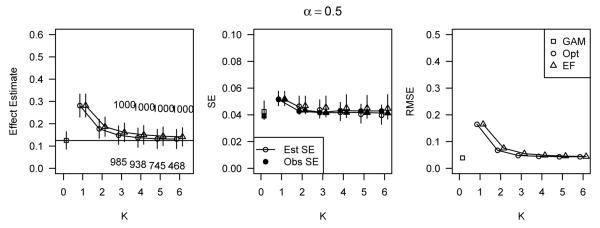
Figure 1 shows the average estimated treatment effect with one observed standard error bars (left panel), observed standard errors and average estimated standard errors with 95% quantile bars (center panel), and observed root MSE (right panel) for data simulated under the additive model with a linear relation between covariates and outcome (relation (A)). Data are displayed for simulations using all three values of α and for all analysis approaches considered. The horizontal axis is K, the number of strata used, where K = 0 refers to the non-stratification method, GAM. When K = 1, there was no stratification (direct estimation through a simple difference of means); these estimates show the amount of initial bias. For K > 2, the number of simulations out of 1000 that had K* = K is printed above the corresponding plotting point for EF stratifications, and below the corresponding point for optimal stratifications.
Figure 1.

Average estimated treatment effect with one observed standard error bars (left panel), observed standard errors and average estimated standard errors with 95% quantile bars (center panel), and observed root MSE (right panel) for data simulated under the additive model with linear relations between covariates and outcome (relations (A)). Data is displayed for simulations using all three values of α and for all analysis approaches considered. The horizontal axis is K, the number of strata used, where K = 0 refers to the use of non-stratification methods (GAM), and K = 1 means no stratification (direct estimation through a simple difference of means).
The effect estimate plots show that the GAM and both stratification approaches were effective at reducing or eliminating bias due to covariate imbalance. In particular, for each value of α, the GAM produced estimates of treatment effect that were on average unbiased. Bias reduction through stratification was achieved better at larger values of K, and consideration of partitions with more than 6 strata could have potentially resulted in unbiased stratified estimates. The optimal stratification method slightly outperformed EF stratification with respect to bias reduction at moderate values of K, but at large values of K, the bias was equivalent for both stratifications (or even slightly favoring EF stratification) and the observed standard error was smaller for EF stratification. The standard error plots in Figure 1 show that our standard error estimator for the stratified treatment effect estimates underestimated the observed standard error on average. Observed standard errors generally increased as K increased. The standard error estimate resulting from the GAM was on average close to the observed standard error and generally lower than the observed standard errors resulting from either stratification approach. The plots of root MSE (RMSE) in Figure 1 show that in these data the GAM resulted in lower RMSE than the stratification approaches, regardless of the value of α. The differences in RMSE between the GAM and stratification approaches became larger as α increased.
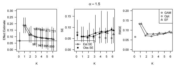
In Figure 2, we display the same information as in Figure 1, except for α = 0.5 only and for covariate-outcome relations (B). The patterns are primarily the same as they were when the covariate-outcome relations were linear. GAM again provided an unbiased estimate with equivalent or smaller observed standard error than either stratification method. Although not shown, the differences in RMSE among estimation methods were again larger at larger values of α. These results, as well as the simulation results for relations (C), are available in Web Supplement B and are similar to the results presented in Figures 1 and 2.
Figure 2.
Simulation results for data simulated under the additive model with α = 0.5 and covariate-outcome relations (B), corresponding to h1(x) = 0.25x and h2(x) = 0.025(x + x3).
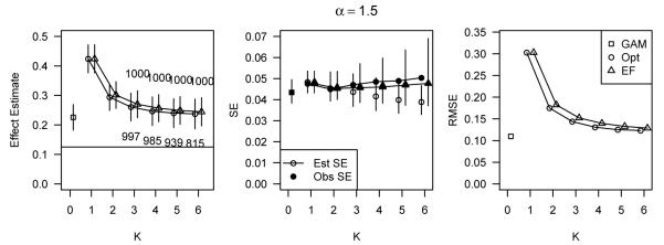
Figure 3 displays simulation results for data simulated under the log-additive model with α = 1.5 and covariate-outcome relations (A). Note that the true ATE in these data is no longer equal to β1 and will vary depending on other simulation parameters. Both the GAM and the stratification approaches with K = 6 estimated the true treatment effect well, but the observed standard errors of the stratified estimators were much larger than that of the GAM estimator, resulting in higher RMSE for the stratified estimators. However, the difference in the estimated standard errors were reversed; the GAM generally overestimated the standard error of the treatment effect estimate, while the standard errors of the stratification estimates were underestimated. Therefore, the average estimated standard error was higher for the GAM compared to the stratification approaches.
Figure 3.
Simulation results for data simulated under the log-additive model with α = 1.5 and covariate-outcome relations (A), corresponding to h1(x) = h2(x) = 0.25x.
In Figure 4, results are shown, as in Figure 3, for the log-additive simulations with α = 1.5 and covariate-outcome relations (B). Results were similar to those with covariate-outcome relations (A) and again show that the GAM generally outperformed stratification. The results for other values of α and the covariate-outcome relations (C) were similar. See the Web Supplement for these results.
Figure 4.
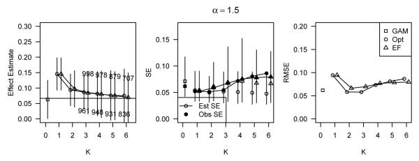
Simulation results for data simulated under the log-additive model with α = 1.5 and covariate-outcome relations (B), corresponding to h1(x) = 0.25x and h2(x) = 0.025(x + x3).
4 Simulation Study: A Poorly-estimated PS
We conducted a second simulation study to compare the performance of methods when the PS is poorly-estimated. We simulated data exactly as in Section 3 and generated outcomes under the additive model (9). In each simulated dataset, we estimated a PS using logistic regression with the covariate X1 only. The estimated PS, (X1), was then used with each of the methods as before.
4.1 Simulation settings
We again considered samples of size N = 200, and we considered the functional forms (B) and (C) from Section 3 for the covariate-outcome relations. The values of all model parameters were identical to those used with the additive model in Section 3, so the ATE is β1 = 0.125.
4.2 Simulation Results
Figure 5 presents the results for the simulation scenario defined by α = 1.5 and covariate-outcome relations (B). The results for other simulation scenarios are not presented here but are similar to those in Figure 5 and are included in the Web Supplement. In general, when the covariate X2 was strongly associated with outcome, as in Figure 5, all methods utilizing the poorly-estimated PS produced highly biased estimates of treatment effect. Although all methods performed poorly, reflecting the unmeasured confounding from X2, the GAM still produced estimates with lower bias and lower RMSE than either stratification method. In addition, the observed standard error of the GAM estimate was generally equal to or lower than the observed standard errors of the stratified estimates.
Figure 5.
Performance of methods applied to a poorly-estimated PS for data simulated under the additive model with α = 1.5, and covariate-outcome relations (B), corresponding to h1(x) = 0.25x and h2(x) = 0.025(x + x3).
5 Analysis of Insurance Plan Choice Data
The following analysis considers data collected on 2515 asthma patients as part of the 1998 Asthma Outcomes Survey (Masland et al., 2000). This study was initiated by the Pacific Business Group on Health and HealthNet health plan for the purpose of evaluating the quality of asthma care from 20 physician groups. Huang et al. (2005) developed PS methods to assess the effect of physician group in a multiple treatment analysis. Because we prefer a binary treatment, our analysis evaluates the effect of health insurance type on satisfaction with asthma care across the 20 providers. Insurance type is classified as public, purchased through an employer, purchased personally, or other. A large majority, 2360 individuals, held either employer or personally purchased health insurance, and we consider the subset of data with these two insurance types. Our treatment variable, Z, indicates having personally purchased health insurance.
The outcome is also dichotomous; Y = 1 indicates very good or excellent satisfaction with care, and Y = 0 indicates less than very good satisfaction. We are interested in estimating the average difference in the probability of high satisfaction with care between individuals with personally purchased and employer purchased insurance plans, controlling for confounders of treatment assignment and outcome. Although the outcome in this example is binary rather than continuous as in the simulation studies, our goal of estimation, the ATE, is the same. Therefore, we followed the suggestion of Hellevik (2008) and applied each PS adjustment method exactly as it was implemented in the simulation studies in Sections 3 and 4.
We began by considering the measured covariates available for use in the PS, which include information about demographics, medical care, and health status. Demographic covariates are age (18-56), race (Black, White, Asian/Pacific Islander, American Indian, Other), Hispanic identification, gender, educational attainment (high school or less, college, post-graduate work), and employment status (none, part-time, full-time). Covariates that describe subjects’ medical care are primary physician specialty (pulmonary/allergy specialist, other), consistent care by the same provider, physician group (1-20), and drug insurance coverage. Health status covariates include smoking (none, moderate, high), physical activity in the last four weeks (1-7), severity of asthma (1-4), comorbidity count (0-8), number of years with asthma (1-54), and the SF36 Health Survey composite scores for physical and mental health (0-100).
We next had to choose which of the measured covariates to include in the PS model. Several simulation studies have found that best results are achieved by only including covariates that are associated with outcome (Austin et al., 2007; Brookhart et al., 2006). This selection will include all of the measured confounders, those covariates associated with both treatment assignment and outcome. Therefore, before we estimated any PS models, we checked each covariate for an independent association with outcome by fitting a logistic regression model of outcome on treatment and the covariate. These models allowed us to order the covariates with respect to their association with outcome, as recommended by Hill (2008). For nominal categorical covariates, we fit logistic GLMs, and for continuous or ordinal categorical covariates, we fit logistic GAMs. Results from these models for the 11 categorical covariates and 6 continuous covariates are displayed in Web Supplement B. From these figures, we determined that only smoking, employment status, and physical activity share no association with the outcome, satisfaction with asthma care, after adjusting for treatment.
In the spirit of flexible model estimation, we used a logistic GAM of the personal health insurance indicator on the remaining 14 covariates that are associated with outcome to estimate the PS for each individual (Woo et al., 2008). The PS obtained is the predicted probability of holding personally purchased insurance, rather than employer purchased insurance, given model covariates. We ran an all subset regression with the eight most important covariates (always present in the model) and some subset of the other six predictors. We compared the unbiased risk estimator (UBRE) of these 64 models to identify a smaller set of useful candidate models. For each candidate model, we then checked the balance of all 14 covariates associated with outcome to identify our final model for propensity score estimation. Balance was checked through side-by-side boxplots of covariates, stratified on both treatment and PS quintile, or through two-by-two tables of treatment and covariates within PS quintiles. Figures in Web Supplement C show the balance checks for the final model chosen, which included: (1) random intercepts for physician groups; (2) main effects for race, education, consistent provider care, drug coverage, years with asthma, physical composite score, and mental composite score; and (3) a smooth term for age, which we note has a nonlinear relation with the log odds of treatment. Older and younger adults are more likely to have personally purchased health insurance than adults in middle-age.
Figure 6 shows the density of the PS in each treatment group. The two groups overlapped well with respect to PS, indicating that ATE can be estimated for the entire PS range. We next applied each of the three methods for estimating treatment effect that were considered in the Monte Carlo studies: GAM regression, EF stratification, and optimal stratification. In addition, we compared these PS-based methods with the usual regression of outcome on the covariates used in the PS model and the treatment indicator.
Figure 6.

Relative frequencies of the estimated PS conditional on treatment. Only 26.4% of individuals had personally purchased health insurance (“Treated”), and 73.6% had employer purchased health insurance (“Untreated”).
Figure 7 displays the treatment effect estimation results of all analysis approaches considered. All methods estimated a positive (but generally not statistically significant) effect of holding personally purchased health insurance on satisfaction with asthma care. In particular, the GAM regression on PS estimated that, on average, the probability of being highly satisfied with asthma care is 0.047 (−0.004, 0.097) higher for individuals with personally purchased health insurance than for individuals with employer purchased health insurance, controlling for propensity to treatment. For individuals with average estimated PS, this risk difference corresponds to 59.8% and 55.1% of individuals highly satisfied with asthma care in the treated and untreated groups, respectively. This estimate is reduced slightly from the unadjusted treatment effect estimate, 0.061 (0.015, 0.107). In Web Supplement C, we show the estimated smooth term for PS as estimated by the GAM. There is a small positive relation between PS and outcome, reflecting the confounding of the treatment-outcome association.
Figure 7.

Treatment effect estimates with confidence intervals, using a regular regression approach (Reg), the GAM regression on the PS approach (GAM), and the optimal (Opt) and equal frequency (EF) stratification on PS approaches.
6 Discussion
The objective of this study was to compare the relative merits of stratification and regression approaches utilizing the PS for estimating treatment effects in nonrandomzied studies and to explore the potential of an ‘optimal’ stratification procedure. Stratification on PS and regression on the PS via GAM both estimated treatment effect flexibly, allowing for nonlinear association between PS and outcome, and both were effective at reducing bias due to confounding. Within the framework of the Monte Carlo simulations presented here, we recommend the GAM approach because it generally produced estimates with lower bias and variance than the stratification approaches. In addition, with cross-validated smoothing parameter selection the GAM depended less on accurate user choice to achieve bias reduction compared with stratification where, at minimum, an appropriate value of K was required. The lack of necessary user choice in GAMs allowed the outcomes to stay “hidden” until the final step of analysis (except for choosing variables to enter the PS model), as advocated by Rubin (2001, 2007). Any attempt to improve on the stratification procedure, as we have done here with our ‘optimal’ stratification, will require using outcome data to choose the partition.
Although the findings presented in this paper are consistent across a wide spectrum of data generating models, our simulation studies do have some limitations. First, the variance estimator that was used for the stratified treatment effect estimates is known to underestimate the variance because it treats the PS partition as fixed, rather than data dependent (D’Agostino Jr., 1998; Tu and Zhou, 2002). Our overall estimation procedure could be bootstrapped to provide a more accurate variance estimate; however, choosing a partition based on the bootstrapped variance estimate is infeasible because it would require estimating a separate bootstrap variance for each potential partition. Second, the variance estimator that we used will be highly variable when sample size is small or when there is poor overlap in PS in some strata. This problem was apparent in the simulation studies when examining the variability of the variance estimator in data with good overlap (α = 0.5) compared to data with poor overlap (α = 1.5). Regardless of this variability, the preference for GAM over stratification with respect to MSE was consistent. Third, the relative importance of the bias and variance components of the total estimation error that was seen in this study is specific to the data generating mechanisms used. In particular, studies with a larger sample size than the N = 200 subjects assumed here will find minimizing bias to be a much more important concern than reducing variance. The GAM estimation procedure was generally preferred to stratification with respect to both bias and variance, so this preference should not depend on sample size.
The benefits of GAMs do not, however, overcome the need for great care in PS analysis. For example, analysts must still check for covariate balance conditional on the estimated PS and for sufficient overlap of treatment groups with respect to PS. In the analysis presented in Section 5, we checked approximate balance of covariates within propensity score quintile, which ensures unconfounding of treatment and outcome within quintile. How best to check for balance when the propensity score will be used in a covariate regression has not been studied. Insufficient overlap of the PS may result in a modified estimand or inappropriate extrapolation, regardless of the PS analysis method used. In each of the simulations presented in this paper, we additionally implemented a GAM that estimated a separate smooth term for PS among treated and untreated subjects. We then estimated average treatment effect using this model to predict the unobserved potential outcomes. We did not present the results from this method in Sections 3 and 4 because the imbalance in the tails of the PS distributions led to inappropriate extrapolation and extremely poor estimates of ATE. The GAM with a single smooth term for PS is partially protected from this kind of extrapolation because the estimated effect of treatment is forced to be constant across the range of the PS. Therefore, treatment effect is estimated primarily from data units that lie in overlapping regions of the PS distributions; in the case of heterogeneous treatment effects, both GAM and stratification procedures may result in an estimand for treatment effect that is different than what the investigator intended.
In addition, although not discussed above, we repeated the simulation experiments using a much smaller sample size of N = 40 with the expectation that the GAM would perform poorly. The GAM estimates were biased and highly variable, but GAM estimation still out-performed both stratification methods. We additionally ran one simulation scenario with a sample size of 10,000 and again found that a modification to sample size did not effect our conclusions. Furthermore, we note that, despite many attempts, we were unable to design a reasonable simulation scenario that resulted in lower RMSE for the stratification methods compared with GAM regression. The two covariate case that we studied provides information on relative performance that will generalize to additional covariates. However, additional studies will provide specific information for other cases. Also, it is possible that regression adjustment may be more problematic when variances differ between treatment groups (Rosenbaum and Rubin, 1983). We investigated this possibility in the log-additive simulation studies, where data were simulated with heteroscedastic errors. The stratification approaches allow for differing variance estimates between treatment groups and across strata. The GAM approach does not model the heteroscedasticity, but still outperformed stratification in these simulations.
Supplementary Material
Acknowledgments
This research was supported by Grant 5T32ES012871 from the U.S. National Institute of Environmental Health Sciences and Grant R01 DK061662 from the U.S. National Institute of Diabetes, Digestive and Kidney Diseases. The authors wish to thank I-Chang Huang and Constantine Frangakis for supplying the data analyzed in this paper.
Contributor Information
Jessica A. Myers, Division of Pharmacoepidemiology and Pharmacoeconomics, Department of Medicine, Brigham and Women’s Hospital and Harvard Medical School, Boston, MA 02120, USA.
Thomas A. Louis, Department of Biostatistics, Bloomberg School of Public Health, Johns Hopkins University, Baltimore, MD 21205, USA
References
- Austin PC, Grootendorst P, Anderson GM. A comparison of the ability of different propensity score models to balance measured variables between treated and untreated subjects: a Monte Carlo study. Statistics in Medicine. 2007;26:734–753. doi: 10.1002/sim.2580. [DOI] [PubMed] [Google Scholar]
- Billewicz W. The efficiency of matched samples: An emperical investigation. Biometrics. 1965;21:623–643. [PubMed] [Google Scholar]
- Brookhart M, Schneeweiss S, Rothman K, Glynn R, Avorn J, Sturmer T. Variable selection for propensity score models. American journal of epidemiology. 2006;163:1149. doi: 10.1093/aje/kwj149. [DOI] [PMC free article] [PubMed] [Google Scholar]
- Byrd R, Lu P, Nocedal J, Zhu C. A limited memory algorithm for bound constrained optimization. SIAM Journal on Scientific Computing. 1995;16:1190–1208. [Google Scholar]
- Cochran WG. The effectiveness of adjustment by subclassification in removing bias in observational studies. Biometrics. 1968;24:295–313. [PubMed] [Google Scholar]
- D’Agostino R., Jr. Propensity score methods for bias reduction in the comparison of a treatment to a non-randomized control group. Statistics in Medicine. 1998;17:2265–2281. doi: 10.1002/(sici)1097-0258(19981015)17:19<2265::aid-sim918>3.0.co;2-b. [DOI] [PubMed] [Google Scholar]
- Dehejia RH, Wahba S. Propensity score-matching methods for nonexperimental causal studies. The Review of Economics and Statistics. 2002;84:151–161. [Google Scholar]
- Hastie T, Tibshirani R. Generalized Additive Models. Chapman & Hall; 1990. [DOI] [PubMed] [Google Scholar]
- Hellevik O. Linear versus logistic regression when the dependent variable is a dichotomy. Quality and Quantity. 2008;43:59–74. [Google Scholar]
- Hill J. Discussion of research using propensity-score matching: Comments on’A critical appraisal of propensity-score matching in the medical literature between 1996 and 2003’by Peter Austin, Statistics in. Statistics in medicine. 2008;27:2055–2061. doi: 10.1002/sim.3245. [DOI] [PubMed] [Google Scholar]
- Huang I, Frangakis C, Dominici F, Diette G, Wu A. Application of a propensity score approach for risk adjustment in profiling multiple physician groups on asthma care. Health Services Research. 2005;40:253–278. doi: 10.1111/j.1475-6773.2005.00352.x. [DOI] [PMC free article] [PubMed] [Google Scholar]
- Hullsiek KH, Louis TA. Propensity score modeling strategies for the causal analysis of observational data. Biostatistics. 2002;2:179–193. doi: 10.1093/biostatistics/3.2.179. [DOI] [PubMed] [Google Scholar]
- Little R, An H. Robust likelihood-based analysis of multivariate data with missing values. Statistica Sinica. 2004;14:949–968. [Google Scholar]
- Masland M, Wu A, Diette G, Dominici F, Skinner E. The 1998 asthma outcomes survey. Pacific Business Group on Health; San Francisco, CA: 2000. [Google Scholar]
- R Development Core Team . R Foundation for Statistical Computing. Vienna, Austria: 2010. R: A Language and Environment for Statistical Computing. ISBN 3-900051-07-0. [Google Scholar]
- Rosenbaum PR, Rubin DB. The central role of the propensity score in observational studies for causal effects. Biometrika. 1983;70:41–55. [Google Scholar]
- — Reducing bias in observational studies using subclassification on the propensity score. Journal of the American Statistical Association. 1984;79:516–524. [Google Scholar]
- — Constructing a control group using multivariate matched sampling methods that incorporate the propensity score. The American Statistician. 1985;39:33–38. [Google Scholar]
- Rubin D. Using propensity scores to help design observational studies: application to the tobacco litigation. Health Services and Outcomes Research Methodology. 2001;2:169–188. [Google Scholar]
- — The design versus the analysis of observational studies for causal effects: parallels with the design of randomized trials. Statistics in medicine. 2007;26:20. doi: 10.1002/sim.2739. [DOI] [PubMed] [Google Scholar]
- Rubin DB. Practical implications of modes of statistical inference for causal effects and the critical role of the assignment mechanism. Biometrics. 1991;47:1213–1234. [PubMed] [Google Scholar]
- Shah B, Laupacis A, Hux J, Austin P. Propensity score methods gave similar results to traditional regression modeling in observational studies: a systematic review. Journal of clinical epidemiology. 2005;58:550–559. doi: 10.1016/j.jclinepi.2004.10.016. [DOI] [PubMed] [Google Scholar]
- Sommer A, Zeger SL. On estimating efficacy from clinical trials. Statistics in Medicine. 1991;10:45–52. doi: 10.1002/sim.4780100110. [DOI] [PubMed] [Google Scholar]
- Tu W, Zhou X. A bootstrap confidence interval procedure for the treatment effect using propensity score subclassification. Health Services and Outcomes Research Methodology. 2002;3:135–147. [Google Scholar]
- Weitzen S, Lapane K, Toledano A, Hume A, Mor V. Principles for modeling propensity scores in medical research: a systematic literature review. Pharmacoepidemiology and Drug Safety. 2004;13:841–853. doi: 10.1002/pds.969. [DOI] [PubMed] [Google Scholar]
- Woo M, Reiter J, Karr A. Estimation of propensity scores using generalized additive models. Statistics in medicine. 2008;27:3805–3816. doi: 10.1002/sim.3278. [DOI] [PubMed] [Google Scholar]
- Wood S. Stable and Efficient Multiple Smoothing Parameter Estimation for Generalized Additive Models. Journal of the American Statistical Association. 2004;99:673–687. [Google Scholar]
- Wood SN. Thin-plate regression splines. Journal of the Royal Statistical Society (B) 2003;65:95–114. [Google Scholar]
Associated Data
This section collects any data citations, data availability statements, or supplementary materials included in this article.