Negotiating Multicollinearity with Spike-and-Slab Priors

Abstract

In multiple regression under the normal linear model, the presence of multicollinearity is well known to lead to unreliable and unstable maximum likelihood estimates. This can be particularly troublesome for the problem of variable selection where it becomes more difficult to distinguish between subset models. Here we show how adding a spike-and-slab prior mitigates this difficulty by filtering the likelihood surface into a posterior distribution that allocates the relevant likelihood information to each of the subset model modes. For identification of promising high posterior models in this setting, we consider three EM algorithms, the fast closed form EMVS version of Rockova and George (2014) and two new versions designed for variants of the spike-and-slab formulation. For a multimodal posterior under multicollinearity, we compare the regions of convergence of these three algorithms. Deterministic annealing versions of the EMVS algorithm are seen to substantially mitigate this multimodality. A single simple running example is used for illustration throughout.

1 Posterior Resolution of the Likelihood

Suppose we observe data that consists of y, an n × 1 response vector, and X = [x₁,…, x_p], an n × p matrix of p potential standardized predictors that are related by a Gaussian linear model

$$f(\mathit{y}|\alpha ,\mathit{\beta },\sigma )={\mathrm{N}}_n(\mathit{X}\mathit{\beta },{\sigma }^2{\mathrm{I}}_n),$$ (1.1)

where β = (β₁,…,β_p) is a p × 1 vector of unknown regression coefficients, and σ is an unknown positive scalar. (We assume throughout that y has been centered at zero to avoid the need for an intercept). For this setup we shall also suppose that only an unknown subset of the coefficients in β are zero, and that the goal is the identification and estimation of this subset. Of particular interest to us will be addressing this problem in the presence of multicollinearity, where it is well known that the maximum likelihood estimator (also the least squares estimator) is an unreliable and unstable estimator of β.

A fundamental Bayesian approach to this variable selection problem is obtained by introducing a “spike-and-slab” Gaussian mixture prior on β. Conditionally on a random vector of binary latent variables γ = (γ₁,…, γ_p)′, γ_i ∈ {0, 1}, this prior is defined by

$$\pi (\mathit{\beta }|\sigma ,\mathit{\gamma })={\mathrm{N}}_p(\mathbf{0},{\sigma }^2{\mathit{D}}_{\mathit{\gamma }}^{1/2}\mathit{R}{\mathit{D}}_{\mathit{\gamma }}^{1/2}),$$ (1.2)

where R is a preset covariance matrix and

$${\mathit{D}}_{\mathit{\gamma }}=\text{diag}\{[(1-{\gamma }_1){\upsilon }_0+{\gamma }_1{\upsilon }_1],\dots ,[(1-{\gamma }_p){\upsilon }_0+{\gamma }_p{\upsilon }_1]\}$$ (1.3)

for 0 ≤ υ₀ < υ₁, George and McCulloch (1993). This prior on β is then combined with suitable priors on α, σ and γ. Typical default choices include the relatively noninuential inverse gamma prior on σ², π(σ²) = IG(ν/2, νλ/2) with ν = λ = 1, and the exchangeable beta-binomial prior on γ, obtained by coupling the iid Benoulli form π(γ | θ) = θ^|γ|(1 − θ)^p−|γ|, $(|\gamma |:={\sum }_{i=1}^p{\gamma }_i)$, with a uniform prior on θ ∈ [0, 1]. We will restrict attention to these choices throughout.

Under (1.2), the β_i components of β are marginally distributed as

$$\pi ({\beta }_i|\sigma ,\gamma )=(1-{\gamma }_i)\mathrm{N}(0,{\sigma }^2{\upsilon }_0)+{\gamma }_i\mathrm{N}(0,{\sigma }^2{\upsilon }_1),$$ (1.4)

a mixture of a “spike distribution” N(0, σ²υ₀) and a “slab distribution” N(0, σ²υ₁). For the purpose of variable selection, the idea is to set υ₀ small and υ₁ large, so that the induced posterior will segregate the β_i coefficients into those that are attributed to the spike distribution and so are inconsequential, and those that are attributed to the slab distribution and so are important. As an alternative to setting υ₁ to be a large fixed value, one may instead add a prior π(υ₁) to induce heavy-tailed slab distributions.

We shall be interested here in considering the effect of the two particular choices, R = I_p and R = (X′X)⁻¹. The choice R = I_p, under which the components of β are independently distributed, serves to decrease the posterior correlation between these components. The g-prior (Zellner, 1986) related choice R = (X′X)⁻¹, which is proportional to the correlation structure of the likelihood estimates of β, serves to reinforce this structure in the posterior. These two choices have opposite effects on the posterior correlation.

After integrating out α, the induced marginal posterior distribution on β is of the form

$$\pi (\mathit{\beta }|\mathit{y})=\sum _{\mathit{\gamma }}\pi (\mathit{\beta }|\mathit{\gamma },\mathit{y})\pi (\mathit{\gamma }|\mathit{y})$$ (1.5)

where the model posterior π(γ | y) puts more weight on those models which are more likely to have generated y. The form of each conditional component of (1.5),

$$\pi (\mathit{\beta }|\mathit{\gamma },\mathit{y})\propto \int L(\mathit{\beta },\sigma |\mathit{y})\pi (\mathit{\beta }|\sigma ,\mathit{\gamma })\pi (\sigma )d\sigma ,$$ (1.6)

shows how the likelihood L(β, σ | y), which does not at all depend on γ, is filtered to determine the distribution of β for each of the subset models determined by γ.

Insight into the effect of the spike-and-slab prior (1.2) on the posterior components through (1.6) is clearest when R = I_p. In this case, L(β, σ | y) is multiplied by

$$\pi (\mathit{\beta }|\sigma ,\mathit{\gamma })=[\prod _{{\gamma }_i=0}{\varphi }_{{\sigma }^2{\upsilon }_0}({\beta }_i)\left]\right[\prod _{{\gamma }_i=1}{\varphi }_{{\sigma }^2{\upsilon }_1}({\beta }_i)],$$ (1.7)

where ϕ_σ²υ(·) is the N(0, σ²υ) density function. Thus, L(β, σ | y) is downweighted when both β_i is large and γ_i = 0. In particular, when υ₀ = 0, L(β, σ | y) is multiplied by 0 when both β_i ≠ 0 and γ_i = 0, effectively conditioning on β_i = 0. In contrast, L(β, σ | y) is relatively unaffected by those β_i for which γ_i = 1, as long as they are not too extreme as determined by υ₁.

The translation of the likelihood information into distinct components via (1.5) facilitates the identification of those submodels best supported by the data. The enhanced clarity provided by the posterior is especially pronounced in the presence of multicollinearity, as illustrated by the simple simulated example described in the next section.

2 Motivating Example with Multicollinearity

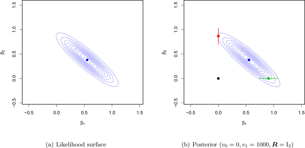
We constructed n = 100 observations on p = 2 predictors according to N_p(0, Σ) with $\mathrm{\Sigma }={({\rho }_{ij})}_{i,j=1}^p$ and ρ_ij = 0.9^|i−j|. Setting β = (1, 0)′, we then generated responses from N_n(Xβ, σ²I_n) with σ² = 3. The resulting maximum likelihood estimate (MLE) β̂_MLE = (0.55, 0.38)′ is at the center of the likelihood surface depicted in Figure 1(a). The instability of the MLE due to the collinearity between the predictors has led it to misallocate the signal across the coordinates.

Figure 1.

Likelihood surface and multimodal posterior landscapes under the point-mass spike-and-slab prior

Now consider what happens when we add the spike-and-slab prior with υ₀ = 0, υ₁ = 1000 and R = I₂. The posterior π(β | y) has translated the likelihood information through (1.5) to the π(γ | y) weighted sum of the four π(β | γ, y) components corresponding to γ = (0, 0)′, (1, 0)′, (0, 1)′, (1, 1)′, respectively. By using υ₀ = 0, which yields a point mass at zero for the spike distribution, these four components support β values of the form (0, 0)′, (β₁, 0)′, (0, β₂)′ and (β₁, β₂)′, respectively.

These components can be identified as the four regions of posterior accumulation in Figure 1(b), which depicts the four posterior modes and associated posterior student-t contours (and 95% HPD intervals for the 1-dimensional regions). The probability mass is distributed among these components according to the posterior model probabilities π[(0, 0)′|y] < 0.001, π[(0, 1)′|y] = 0.187, π[(1, 0)′ | y] = 0.764 and π[(1, 1)′ | y] = 0.049. The global mode β̂_MAP = (0.91, 0.00)′, a much better estimate than the MLE, is sitting atop the (β₁, 0) component, which has been most heavily weighted by π(γ | y) for this data. We note in passing that replacing R = I₂ by R = (X′X)⁻¹ here, yields virtually the same posterior as in Figure 1(b).

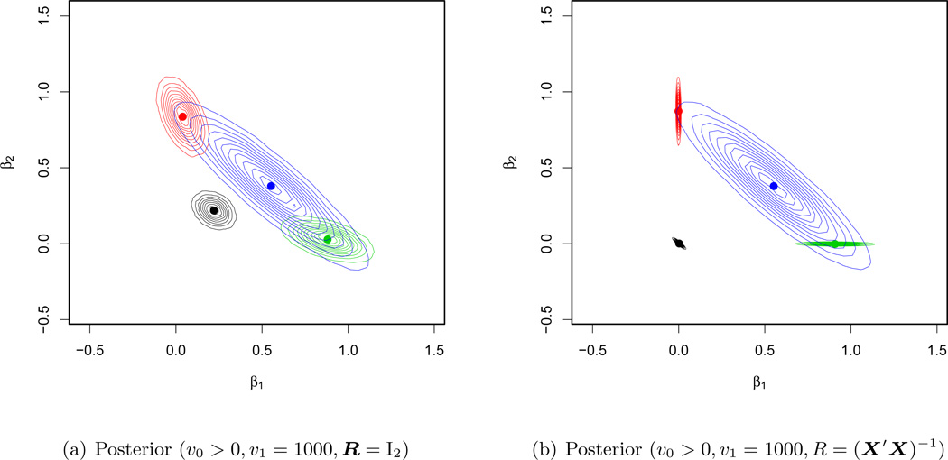
It will also be of interest to get some insight into the effect of using υ₀ > 0, so let us also consider what happens when we change υ₀ = 0 to υ₀ = 0.005 in the above. As before, the posterior π(β | y) is the weighted sum of the four π(β | γ, y) components corresponding to γ = (0, 0)′, (1, 0)′, (0, 1)′, (1, 1)′, respectively. However because υ₀ > 0 employs a continuous spike distribution, none of these posterior components rule out any β values. Instead, the first three posterior components are distinguished only by more heavily weighting β values close to (0, 0)′, (β₁, 0)′, (0, β₂)′.

Under the independence prior choice R = I₂, these components can still be identified as the four regions of posterior accumulation in Figure 2(a). However, in contrast to Figure 1(b), they are now all full dimensional and not quite as cleanly separated. Nonetheless, the global mode β̂_MAP = (0.88, 0.03)′, is still a much better estimate than the MLE, sitting atop the γ = (1, 0)′ component, which again has been most heavily weighted by π(γ | y) for this data. This posterior has still been effective at mitigating the effect of multicollinearity.

Figure 2.

Posterior landscapes under continuous spike and slab priors

When we instead consider the g-prior choice R = (X′X)⁻¹, it is interesting to see how the posterior π(β | y), now depicted in Figure 2(b), has changed. The four components now appear as an intermediate change between the υ₀ = 0 posterior in Figure 1(b) and the υ₀ > 0 posterior in Figure 2(a). The g-prior structure has served to maintain the multicollinear structure in the components corresponding to γ = (0, 0)′, (1, 0)′, (0, 1)′, keeping them more similar to their lower dimensional counterparts in Figure 1(b). With this posterior, the global mode β̂_MAP = (0.901, 0.001)′ is now even closer to the true β = (1, 0)′.

3 EM Algorithms for Posterior Mode Identification

As a practical matter, identification of the posterior mode under the spike-and-slab prior formulation can be challenging when the number of predictors is large. For this purpose, EM algorithms can provide a fast deterministic search alternative to stochastic search approaches such as SSVS George and McCulloch (1993, 1997). In this section, we describe three such EM algorithms which are designed for different choices of υ₀ and R. The first of these was proposed by Rockova and George (2014) (hereafter RG14) for (υ₀ > 0, R = I_p), involving closed form E-step and M-step updates. The other two are new algorithms designed for the cases (υ₀ > 0, R = (X′X)⁻¹) and (υ₀ = 0, R = I_p), respectively, and exploit mean-field approximations in the E-step.

The EM algorithm has been previously considered in the context of Bayesian shrinkage estimation under sparsity priors (Figueiredo (2003)), Kiiveri (2003), Griffin and Brown (2012, 2005). Literature on similar computational procedures for spike-and-slab models is far more sparse. EM-like algorithms for point mass variable selection priors were considered by Hayashi and Iwata (2010) and Bar et al. (2010), which approximate the E-step by neglecting the correlation among the selection indicators. The EM algorithm for the point mass prior that we describe below uses a mean-field approximated E-step, which takes into account the fact that the selection indicators can be dependent. A similar dependence also occurs in the case (υ₀ > 0 and R = (X′X)⁻¹). There we again take advantage of the mean field approximation, which induces “dependent thresholding” for variable selection rather than univariate thresholding along individual coordinate axes.

3.1 The EMVS Algorithm for υ₀ > 0 and R = I_p

For the problem of model identification, RG14 proposed EMVS, an approach based on a fast closed form EM algorithm that quickly identifies posterior modes of π(β, θ, σ² |y) under a spike-and-slab prior with υ₀ > 0 and R = I_p. The modal β values are then thresholded to identify nearby high posterior γ models under the posterior for which υ₀ = 0. We refer to this EM algorithm as the EMVS algorithm.

As described in detail in RG14, the EMVS algorithm proceeds by iteratively maximizing the objective function

$$Q(\mathit{\beta },\theta ,\sigma |{\psi }^{(k)})=-\frac{{\Vert \mathit{y}-\mathit{X}\mathit{\beta }\Vert }^2}{2{\sigma }^2}-\text{log}{\sigma }^{n-1+p+\nu }-\frac{\nu \lambda }{2{\sigma }^2}-\frac{1}{2{\sigma }^2}\sum _{i=1}^p{\beta }_i^2{𝖤}_{\mathit{\gamma }|·}[\frac{1}{{\upsilon }_0(1-{\gamma }_i)+{\upsilon }_1{\gamma }_i}]+\sum _{i=1}^p\text{log}(\frac{\theta }{1-\theta }){𝖤}_{\mathit{\gamma }|·}[{\gamma }_i]+p\text{log}(1-\theta ),$$ (3.1)

where ψ^(k) = (β^(k), θ^(k), σ^(k)) and 𝖤_γ|·[·] denotes expectation conditionally on [ψ^(k), y]. At the kth iteration, an E-step is first applied, computing the expectations in (3.1), followed by an M-step that maximizes over (β, θ, σ) to yield the values of ψ^(k+1) = (β^(k+1), θ^(k+1), σ^(k+1)).

The E-step expectations are obtained quickly from the closed form expressions

$${𝖤}_{\mathit{\gamma }|·}[{\gamma }_i]=\frac{\pi ({\beta }_i^{(k)}|{\sigma }^{(k)},{\gamma }_i=1){\theta }^{(k)}}{\pi ({\beta }_i^{(k)}|{\sigma }^{(k)},{\gamma }_i=1){\theta }^{(k)}+\pi ({\beta }_i^{(k)}|{\sigma }^{(k)},{\gamma }_i=0)(1-{\theta }^{(k)})}\equiv p_i^{★}$$ (3.2)

and

$${𝖤}_{\mathit{\gamma }|·}\left[\frac{1}{{\upsilon }_0(1-{\gamma }_i)+{\upsilon }_1{\gamma }_i}\right]=\frac{1-p_i^{★}}{{\upsilon }_0}+\frac{p_i^{★}}{{\upsilon }_1}\equiv d_i^{★}.$$ (3.3)

Note that these closed form expressions are available when υ₀ > 0 but not when υ₀ = 0.

For the M-step maximization, the β^(k+1) value that globally maximizes Q is obtained by the generalized ridge estimator

$${\mathit{\beta }}^{(k+1)}={(\mathit{X}\prime \mathit{X}+{\mathit{D}}^{★})}^{-1}\mathit{X}\prime \mathit{y}$$ (3.4)

where ${\mathit{D}}^{★}=\text{diag}{\{d_i^{★}\}}_{i=1}^p$ is the p × p diagonal matrix with entries $d_i^{★}>0$, the well-known solution to the ridge regression problem

$${\mathit{\beta }}^{(k+1)}={\text{argmin}}_{\mathit{\beta }\in {ℝ}^p}\{{\Vert \mathit{y}-\mathit{X}\mathit{\beta }\Vert }^2+{\Vert {\mathit{D}}^{★1/2}\mathit{\beta }\Vert }^2\}.$$ (3.5)

In problems where p >> n, the calculation of (3.4) can be enormously reduced by using the Sherman-Morrison-Woodbury formula to obtain an expression which requires a n × n matrix inversion rather than a p × p matrix inversion. Alternatively, as described in George et al. (2013), the solution of (3.5) can be obtained even faster with the stochastic dual coordinate ascent algorithm of Shalev-Shwartz and Zhang (2013).

The maximization of Q is then completed with the simple updates

$${\sigma }^{(k+1)}=\sqrt{\frac{{\Vert \mathit{y}-\mathit{X}{\mathit{\beta }}^{(k+1)}\Vert }^2+{\Vert {\mathit{D}}^{★1/2}{\mathit{\beta }}^{(k+1)}\Vert }^2+\nu \lambda }{n+p+\nu }}$$ (3.6)

and

$${\theta }^{(k+1)}=\frac{1}{p}\sum _{i=1}^p{p}_i^{*}.$$ (3.7)

3.2 An Approximate EM Algorithm when υ₀ > 0 and R = (X′X)⁻¹

When υ₀ > 0 and R = (X′X)⁻¹, an EM algorithm with a fast closed form E-step is no longer available. However, as we now show, an EM algorithm for variable selection becomes feasible with deterministic mean field approximations.

The expectation of the complete data log-likelihood here requires computation of both the first and second moments of the vector of latent γ indicators. This is better seen from the following expression for the objective function

$$Q(\mathit{\beta },\theta ,\sigma |{\psi }^{(k)})=-\frac{{\Vert \mathit{y}-\mathit{X}\mathit{\beta }\Vert }^2}{2{\sigma }^2}-\text{log}{\sigma }^{n-1+p+\nu }-\frac{\nu \lambda }{2{\sigma }^2}-\frac{{𝖤}_{\mathit{\gamma }|·}[\mathit{\beta }\prime {\mathit{D}}_{\gamma }^{-1/2}\mathit{X}\prime \mathit{X}{\mathit{D}}_{\gamma }^{-1/2}\mathit{\beta }]}{2{\sigma }^2}+\sum _{i=1}^p\text{log}(\frac{\theta }{1-\theta }){𝖤}_{\mathit{\gamma }|·}[{\gamma }_i]+p\text{log}(1-\theta ).$$ (3.8)

The expectation of the quadratic form in the fourth summand can be written as

$${𝖤}_{\mathit{\gamma }|·}[\mathit{\beta }\prime {\mathit{D}}_{\gamma }^{-1/2}\mathit{X}\prime \mathit{X}{\mathit{D}}_{\gamma }^{-1/2}\mathit{\beta }]={(\frac{1}{\sqrt{{\upsilon }_1}}-\frac{1}{\sqrt{{\upsilon }_0}})}^2\text{tr}\{\text{diag}\{\mathit{\beta }\}\mathit{X}\prime \mathit{X}\text{diag}\{\mathit{\beta }\}{𝖤}_{\mathit{\gamma }|·}\mathit{\gamma }\mathit{\gamma }\prime \}$$ (3.9)

$$+\frac{2}{\sqrt{{\upsilon }_0}}(\frac{1}{\sqrt{{\upsilon }_1}}-\frac{1}{\sqrt{{\upsilon }_0}}){𝖤}_{\mathit{\gamma }|·}\mathit{\gamma }\prime \text{diag}\{\beta \}\mathit{X}\prime \mathit{X}\mathit{\beta }+\frac{1}{{\upsilon }_0}\mathit{\beta }\prime \mathit{X}\prime \mathit{X}\mathit{\beta }.$$ (3.10)

The first and second conditional moments of γ above are with respect to the following conditional distribution which, based on (1.2), resembles a Markov Random Field (MRF) distribution on a completely connected graph with self-loops, i.e.

$$\pi (\mathit{\gamma }|{\mathit{\psi }}^{(k)})\propto \text{exp}\{\mathit{\gamma }\prime \mathit{a}+\mathit{\gamma }\prime B\mathit{\gamma }\},$$ (3.11)

where

$$\mathit{a}=-\frac{1}{{\sigma }^{(k)2}}\left(\frac{\sqrt{{\upsilon }_0}-\sqrt{{\upsilon }_1}}{\sqrt{{\upsilon }_1}{\upsilon }_0}\right)\text{diag}\{{\mathit{\beta }}^{(k)}\}\mathit{X}\prime \mathit{X}{\mathit{\beta }}^{(k)}+\left[\frac{1}{2}\text{log}\right(\frac{{\upsilon }_0}{{\upsilon }_1})+\text{log}(\frac{{\theta }^{(k)}}{1-{\theta }^{(k)}}\left)\right]\mathbf{1}$$ (3.12)

and

$$\mathit{B}=-\frac{1}{2{\sigma }^{(k)2}}{(\frac{1}{\sqrt{{\upsilon }_1}}-\frac{1}{\sqrt{{\upsilon }_0}})}^2\text{diag}\{{\mathit{\beta }}^{(k)}\}\mathit{X}\prime \mathit{X}\text{diag}\{{\mathit{\beta }}^{(k)}\}.$$ (3.13)

Note that the distribution (3.11) deviates slightly from a traditional MRF distribution, which assumes that the matrix B has zeroes on the diagonal. Nevertheless, the exact computation of 𝖤_γ|·γ and 𝖤_γ|·γγ′ is still feasible in small problems. However, for applications involving moderate to large numbers of predictors, approximate computation will be needed.

It is interesting to point out the effect of the g-prior on simultaneously selecting variables that are related. For standardized predictors, X′X is proportional to the sample correlation matrix. A pair (i, j) of highly collinear predictors will have a large entry (X′X)_(i,j) in absolute value, which can be potentially magnified by the current parameter estimates ${\beta }_i^{(k)}$ and ${\beta }_j^{(k)}$. For example, for large positive (X′X)_(i,j), large ${\beta }_i^{(k)}$ and ${\beta }_j^{(k)}$ of the same sign will lead to a large negative B_(i,j) entry, which will in turn lower their probability of co-occurence at the kth iteration.

3.2.1 Mean Field Approximated E-step

For the E-step calculations, we deploy a variant of a mean field approximation which outputs approximations to 𝖤_γ|·γ_i for i = 1,…, p as a solution to a series of nonlinear equations. Proceeding as in RG14, the approximations 𝖤̂_γ|·γ_i = μ_i can be obtained by solving

$${\mu }_i=\frac{\text{exp}(a_i+{\sum }_{j=1}^p{B}_{ij}{\mu }_j)}{1+\text{exp}(a_i+{\sum }_{j=1}^p{B}_{ij}{\mu }_j)},\text{for}i=1,\dots ,p.$$

Because the vector a and matrix B can involve rather large numbers, it will be useful in practice to perform the approximation with reparametrized values a★ = a/C and B★ = B/C² to obtain ${\mu }_i^{★}$. The solution can be transformed back by noting $\text{logit}({\mu }_i)=C\text{logit}({\mu }_i^{★})$. The constant C can be for instance chosen as the maximum of the absolute value of the entries in the matrix B and the vector a. The matrix of second posterior moments can then be approximated by 𝖤̂_γ|·[γγ′] = 𝖤̂_γ|·[γ]𝖤̂_γ|·[γ′], because the approximating distribution assumes a completely disconnected graph.

3.2.2 The M-step

The M-step proceeds by jointly updating (β,σ,θ), which is equivalent to updating (β,σ) and θ individually. Only the updates for the regression parameters and residual variance require slight modification:

$${\mathit{\beta }}^{(k+1)}={[\mathit{X}\prime \mathit{X}+{\mathit{D}}^{★1/2}\mathit{X}\prime \mathit{X}{\mathit{D}}^{★1/2}]}^{-1}\mathit{X}\prime \mathit{y},$$

and

$${\sigma }^{(k+1)}=\sqrt{\frac{{\Vert \mathit{y}-\mathit{X}{\mathit{\beta }}^{(k+1)}\Vert }^2+{\Vert {\mathit{\beta }}^{(k+1)\prime }{\mathit{D}}^{★1/2}\mathit{X}\prime \mathit{X}{\mathit{D}}^{★1/2}{\mathit{\beta }}^{(k+1)}\Vert }^2+\nu \lambda }{n-1+p+\nu }}.$$

3.3 An Approximate EM Algorithm when υ₀ = 0 and R = I_p

We now describe a variant of the EM algorithm for the point-mass prior (υ₀ = 0), assuming that the covariates are a priori independent (R = I_p). Here, the joint prior distribution (1.2) is degenerate for all models of dimension smaller than p.

Our derivation proceeds by first rewriting the likelihood for every model γ as

$$f(\mathit{y}|\mathbf{\Gamma },\mathit{\beta },\sigma )={\mathrm{N}}_n(\mathit{X}\mathbf{\Gamma }\mathit{\beta },{\sigma }^2{\mathrm{I}}_n),$$ (3.14)

where $\mathbf{\Gamma }=\text{diag}{\{{\gamma }_i\}}_{i=1}^p$. The objective function for the EM algorithm then becomes

$$Q(\mathit{\beta },\theta ,\sigma |{\mathit{\psi }}^{(k)})=-\frac{{𝖤}_{\mathit{\gamma }|·}{\Vert \mathit{y}-\mathit{X}\mathbf{\Gamma }\mathit{\beta }\Vert }^2}{2{\sigma }^2}-\text{log}{\sigma }^{n-1+\sum {𝖤}_{\mathit{\gamma }|·}[{\gamma }_i]+\nu }-\frac{\nu \lambda }{2{\sigma }^2}-\frac{{𝖤}_{\mathit{\gamma }|·}[\mathit{\beta }\prime \text{diag}\{{\gamma }_i\}\mathit{\beta }]}{2{\sigma }^2{\upsilon }_1}+\sum _{i=1}^p\text{log}(\frac{\theta }{1-\theta }){𝖤}_{\mathit{\gamma }|·}[{\gamma }_i]+p\text{log}(1-\theta ),$$ (3.15)

The expectation of the quadratic form in the first summand can be written as

$${𝖤}_{\mathit{\gamma }|·}{\Vert \mathit{y}-\mathit{X}\mathbf{\Gamma }\mathit{\beta }\Vert }^2=-\frac{1}{2{\sigma }^2}\text{tr}\{\text{diag}\{\mathit{\beta }\}\mathit{X}\prime \mathit{X}\text{diag}\{\mathit{\beta }\}{𝖤}_{\mathit{\gamma }|·}\mathit{\gamma }\mathit{\gamma }\prime \}+\frac{1}{{\sigma }^2}{𝖤}_{\mathit{\gamma }|·}\mathit{\gamma }\prime \text{diag}\{\mathit{\beta }\}\mathit{X}\prime \mathit{Y}-\frac{1}{2{\sigma }^2}\mathit{y}\prime \mathit{y}.$$

As in the EM algorithm for the g-prior, we compute the first and second posterior moments of the latent inclusion indicators. The E-step can again be obtained with a mean field approximation, this time using a slightly different MRF distribution

$$\pi (\mathit{\gamma }|{\mathit{\psi }}^{(k)})\propto \text{exp}\{\mathit{\gamma }\prime \mathit{a}+\mathit{\gamma }\prime B\mathit{\gamma }\},$$ (3.16)

where

$$\mathit{a}=\frac{1}{{\sigma }^{(k)2}}\text{diag}\{{\mathit{\beta }}^{(k)}\}\mathit{X}\prime \mathit{Y}-\frac{1}{2{\sigma }^{(k)2}{\upsilon }_1}\text{diag}\{{\mathit{\beta }}^{(k)}\}{\mathit{\beta }}^{(k)}+\left[\frac{1}{2}\text{log}\right(\frac{1}{{\upsilon }_1})+\text{log}(\frac{{\theta }^{(k)}}{1-{\theta }^{(k)}}\left)\right]\mathbf{1}$$ (3.17)

and

$$\mathit{B}=-\frac{1}{2{\sigma }^{(k)2}}\text{diag}\{{\mathit{\beta }}^{(k)}\}\mathit{X}\prime \mathit{X}\text{diag}\{{\mathit{\beta }}^{(k)}\}.$$ (3.18)

Focusing on the vector of sparsity parameters a, negative parameters ${\beta }_i^{(k)}$ for covariates, which correlate positively with the outcome, induce smaller baseline inclusion probabilities exp(a_i)/[1+ exp(a_i)]. This behavior will become more evident from the plots of convergence regions in the next section.

The M-step update of the joint vector of regression coefficients

$${\mathit{\beta }}^{(k+1)}={({𝖤}_{\mathit{\gamma }|·}\mathbf{\Gamma }\mathit{X}\prime \mathit{X}{𝖤}_{\mathit{\gamma }|·}\mathbf{\Gamma }+{\mathit{D}}^{★})}^{-1}\mathit{X}\prime \mathit{Y}$$

can be unstable, when entries in the approximated 𝖤_γ|·[Γ] approach zero. In such instances, it will be useful to set ${\beta }_i^{(k)}$ directly to zero, when the conditional inclusion probability is smaller than a pre-specified threshold. This sparsification step induces more stability, while rendering the exclusion of each covariate throughout the iterations reversible.

The residual variance is then updated according to

$${\sigma }^{(k+1)}=\sqrt{\frac{{\Vert \mathit{y}-\mathit{X}{𝖤}_{\mathit{\gamma }|·}\mathbf{\Gamma }{\mathit{\beta }}^{(k+1)}\Vert }^2+{\Vert {\mathit{\beta }}^{(k+1)\prime }{\mathit{D}}^{★}{\mathit{\beta }}^{(k+1)}\Vert }^2+\nu \lambda }{n-1+\sum {𝖤}_{\mathit{\gamma }|·}{\gamma }_i+\nu }}.$$

4 Geometry of EM Convergence Regions

Despite attractive features such as rapid convergence, economy of storage and computational speed, our EM algorithms may converge to local modes rather than the global mode of main interest. Overcoming this tendency can be especially challenging in multimodal posterior landscapes, such as those induced by our spike-and-slab priors, where performance becomes heavily dependent on the choice of a starting value. To shed some light on the extent to which this occurs with our EM algorithms, we studied this aspect of their performance on the simple example with two correlated predictors from Section 2. Note that the posterior multimodality there has been exacerbated by the strong collinearity between the predictors.

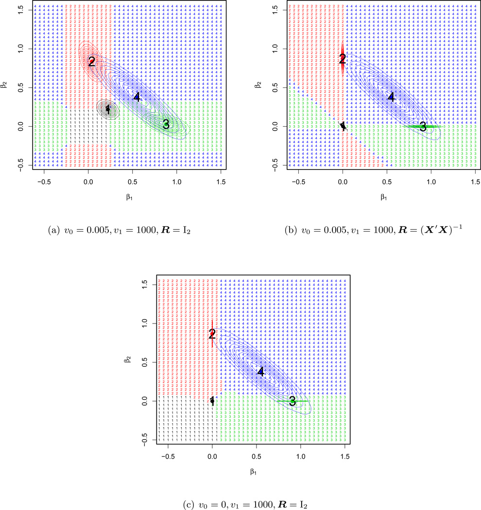
For a regular grid of values on [−0.5, 1.5] × [−0.5, 1.5], we ran each of our three EM algorithms, starting at each point on the grid and recording the mode to which the algorithm converged. These results are displayed in Figure 3(a) for υ₀ = 0.005 and υ₁ = 1000 with R = I₂, in Figure 3(b) for υ₀ = 0.005 and υ₁ = 1000 with R = (X′X)⁻¹ and in Figure 3(c) for υ₀ = 0 and υ₁ = 1000 with R = I₂. Numbering the modes 1, 2, 3 and 4, each starting value has been assigned same number as its EM destination mode. This results in a partition of the grid into four regions, delineating the regions of attraction for each mode.

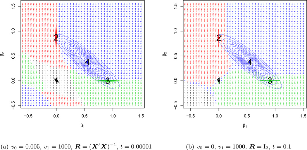
Figure 3.

Geometry of EM convergence regions

These three figures confirm the susceptibility of the EM algorithms to starting values. The convergence towards the global mode (here mode 3) is not guaranteed unless the starting value belongs to the small region of attraction around it. The geometry of the convergence regions differs depending on the variant of our EM algorithm. The independence covariance matrix R = I₂ yields nearly rectangular regions corresponding to thresholding univariate directions. The point-mass prior υ₀ = 0 penalizes the directions of sign inconsistency between the starting value and the sample correlation between the variable and the response. The g-prior R = (X′X)⁻¹ performs dependent thresholding along multivariate directions, rather than coordinate axes.

5 Mitigating Multimodality with Deterministic Annealing

In order to increase the chances of converging to the global mode, Ueda and Nakano (1998) propose a deterministic annealing EM variant (DAEM) based on the principle of maximum entropy and an analogy with statistical mechanics. In our context, the DAEM algorithm aims at finding a maximum of the negative of the free energy function $H_t(\mathit{\beta },\mathit{\theta },\sigma )=\frac{1}{t}\text{log}{\sum }_{\mathit{\gamma }}\pi {(\mathit{\beta },\mathit{\theta },\sigma ,\mathit{\gamma }|\mathit{y})}^t$ where 0 < t < 1. The problem of optimizing the logarithm of the incomplete posterior distribution is embedded as a special case for t = 1.

The parameter 1/t corresponds to a temperature parameter and determines the degree of separation between the multiple modes of F_t(·). Large enough values smooth the function to have only one minimum. As the temperature decreases, multiple modes begin to appear and the function gradually resembles the true log incomplete posterior. The influence of poorly chosen starting values can be weakened by keeping the temperature high at the early stage of computation, gradually decreasing it during the iteration process. Alternatively, the free energy function can be optimized for a decreasing sequence of temperature levels 1/t₁ > 1/t₂ > ⋯ > 1/t_k, where the solution at 1/t_i serves as the starting point for the computation at 1/t_i+1. Provided that the new global maximum is close to the previous one, this strategy can increase the chances of finding the true global maximum. We will investigate how the tempering affects the ability to converge towards the region of attraction of the global mode.

While the M-step of the DAEM algorithm remains unchanged, the E-step requires the computation of the expected complete log posterior density with respect to a distribution which is proportional to the current estimate of the conditional complete posterior given the observed data raised to the power t. This distribution is particularly easy to derive for mixtures (Ueda and Nakano, 1998). We begin by describing this distribution for the EMVS algorithm with υ₀ > 0 and R = I_p, in which case this corresponds to a Bernoulli distribution with inclusion probabilities

$$p_i^{t★}=\frac{\pi {({\beta }_i|{\sigma }^{(k)},{\gamma }_i=1)}^t𝖯{({\gamma }_i=1|{\mathit{\theta }}^{(k)})}^t}{\pi {({\beta }_i|{\sigma }^{(k)},{\gamma }_i=1)}^t𝖯{({\gamma }_i=1|{\mathit{\theta }}^{(k)})}^t+\pi {({\beta }_i|{\sigma }^{(k)},{\gamma }_i=0)}^t𝖯{({\gamma }_i=0|{\mathit{\theta }}^{(k)})}^t}.$$ (5.1)

The EMVS algorithm with annealing then proceeds by substituting (5.1) for (3.2). At high temperatures (t close to zero) the probabilities (5.1) become nearly uniform distribution. This leads to a nearly equal penalty on all the coefficients regardless of their magnitude (the diagonal elements of the ridge matrix equal $\frac{{\upsilon }_0{p}_i^{t★}+{\upsilon }_1(1-p_i^{t★})}{{\upsilon }_1{\upsilon }_0}\approx \frac{{\upsilon }_0+{\upsilon }_1}{2{\upsilon }_0\upsilon 1}$, inducing a unimodal posterior.

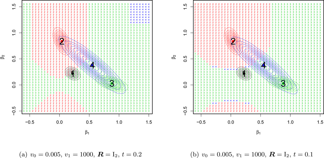
To gauge the effectiveness of deterministic annealing on the EMVS algorithm for υ₀ = 0.005 and υ₁ = 1000 with R = I₂, we recomputed the domains of attraction for t = 0.2 in Figure 4(a) and for t = 0.1 in Figure 4(b) for our simple example. Comparison with from Figure 3(a) shows how annealing has dramatically improved the geometry of the convergence regions. By substantially increasing the region of attraction towards the best mode (number 3), annealing has here increased the chances of converging to the global solution.

Figure 4.

Geometry of convergence regions using deterministic annealing.

Deterministic annealing for the case of the g-prior (υ₀ > 0, R = (X′X)⁻¹) and the point-mass prior (υ₀ = 0, υ₁ = 1000, R = I₂) proceeds by finding the marginals of a MRF distribution, raised to the power of the inverse temperature parameter

$${\pi }^t(\mathit{\gamma }|{\mathit{\psi }}^{(k)})\propto \text{exp}\{t\mathit{\gamma }\prime \mathit{a}+t\mathit{\gamma }\prime B\mathit{\gamma }\}.$$ (5.2)

The mean field approximation can be used just as before (Section 3.2.1), but with the sparsity and connectivity matrix multiplied by t. However, because the entries in both a and B can be prohibitively large, the tempering here will only be effective for very small t. This is particularly true for the continuous g-prior, where both a and B involve quantities depending on 1/υ₀, which can be very large.

The effectiveness of deterministic annealing for these two EM algorithms is displayed in Figure 5. Applied to our simple example, deterministic annealing has not been very effective in increasing the region of attraction toward the global mode.

Figure 5.

Geometry of convergence regions using deterministic annealing.

6 Discussion

We have illustrated how the destabilizing inuence of multicollinearity in variable selection problems can be mitigated by introducing a spike-and-slab prior. Such priors induce posteriors which filter the likelihood information into a weighted sum of cleanly separated posterior modes corresponding to subset models. In order to locate the highest posterior mode, we presented three variants of EM algorithms for variable selection and considered the geometry of their convergence regions in multimodal landscapes. Whereas multicollinearity induces diffculties when using point-mass priors or dependent prior covariances, the EMVS algorithm for a continuous spike-and-slab prior with an independent prior covariance matrix fares superbly when coupled with deterministic annealing.

References

- Bar H, Booth J, Wells M. An Empirical Bayes Approach to Variable Selection and QTL Analysis. In the Proceedings of the 25th International Workshop on Statistical Modelling, Glasgow, Scotland. 2010:63–68. [Google Scholar]
- Figueiredo MA. Adaptive Sparseness for Supervised Learning. IEEE Transactions on Pattern Analysis and Machine Intelligence. 2003;25:1150–1159. [Google Scholar]
- George EI, McCulloch RE. Variable Selection Via Gibbs Sampling. Journal of the American Statistical Association. 1993;88:881–889. [Google Scholar]
- George EI, McCulloch RE. Approaches for Bayesian Variable Selection. Statistica Sinica. 1997;7:339–373. [Google Scholar]
- George E, Rockova V, Lesaffre E. Faster spike-and-slab variable selection with dual coordinate ascent EM. Proceedings of the 28thWorkshop on Statistical Modelling. 2013;1:165–170. [Google Scholar]
- Griffin J, Brown P. Alternative Prior Distributions for Variable Selection with Very Many More Variables Than Observations. Technical report, University of Warwick, University of Kent; 2005. [Google Scholar]
- Griffin JE, Brown PJ. Bayesian Hyper-LASSOS with Non-convex Penalization. Australian & New Zealand Journal of Statistics. 2012;53:423–442. [Google Scholar]
- Hayashi T, Iwata H. EM Algorithm for Bayesian Estimation of Genomic Breeding Values. BMC Genetics. 2010;11:1–9. doi: 10.1186/1471-2156-11-3. [DOI] [PMC free article] [PubMed] [Google Scholar]
- Kiiveri H. A Bayesian Approach to Variable Selection When the Number of Variables is Very Large. Institute of Mathematical Statistics Lecture Notes-Monograph Series. 2003;40:127–143. [Google Scholar]
- Rockova V, George E. EMVS: The EM approach to Bayesian Variable Selection. Journal of the American Statistical Association. 2014 [Google Scholar]
- Shalev-Shwartz S, Zhang T. Stochastic dual coordinate ascent methods for regularized loss minimization. Journal of Machine Learning Research. 2013;14:567–599. [Google Scholar]
- Ueda N, Nakano R. Deterministic Annealing EM Algorithm. Neural Networks. 1998;11:271–282. doi: 10.1016/s0893-6080(97)00133-0. [DOI] [PubMed] [Google Scholar]
- Zellner A. On assessing prior distributions and Bayesian regression analysis with g-prior distributions. Studies in Bayesian Econometrics and Statistics. 1986 [Google Scholar]