Signed directed acyclic graphs for causal inference

Summary

Formal rules governing signed edges on causal directed acyclic graphs are described in this paper and it is shown how these rules can be useful in reasoning about causality. Specifically, the notions of a monotonic effect, a weak monotonic effect and a signed edge are introduced. Results are developed relating these monotonic effects and signed edges to the sign of the causal effect of an intervention in the presence of intermediate variables. The incorporation of signed edges into the directed acyclic graph causal framework furthermore allows for the development of rules governing the relationship between monotonic effects and the sign of the covariance between two variables. It is shown that when certain assumptions about monotonic effects can be made then these results can be used to draw conclusions about the presence of causal effects even when data is missing on confounding variables.

1. Introduction

With very few exceptions (Lauritzen and Richardson, 2002), the use of graphical models in the field of causal inference has been restricted to directed acyclic graphs and graphs allowing for bidirected edges which represent unobserved common causes. The directed acyclic graph causal framework allows for the representation of causal and counterfactual relations amongst variables (Pearl, 1995; Robins, 1997; Pearl, 2000); the estimation of causal effects through the g-formula (Robins, 1986, 1987; Spirtes et al., 1993; Pearl, 1993); the detection of independencies through the d-separation criterion (Verma and Pearl, 1988; Geiger et al., 1990; Lauritzen et al., 1990); and the implementation of algorithms to determine whether conditioning on a particular set of variables, or none at all, is sufficient to control for confounding as well as algorithms which identify such a set of variables (Pearl 1995; Galles and Pearl, 1995; Pearl and Robins, 1995; Kuroki and Miyakawa, 1999, 2003; Geng et al., 2002; Tian and Pearl, 2002).

This paper introduces into the directed acyclic graph causal framework the notion of a monotonic effect along with its graphical counterpart, a signed edge. Considerations of monotonicity have been incorporated into many types of graphical models (Wellman, 1990; Archer and Wang, 1993; Druzdzel and Henrion, 1993; Bioch, 1998; Potharst and Feelders, 2002; van der Gaag et al., 2004). Here our focus will be the causal interpretation of monotonicity relationships within the directed acyclic graph causal framework. We will say that some variable has a positive (or negative) monotonic effect on another if intervening to increase the former will never for any individual decrease (or increase) the latter. We furthermore provide a weaker set of conditions, which we express in terms of weak monotonic effects, related to Wellman’s (1990) "qualitative influence," under which the major theorems presented still hold. By incorporating these notions of monotonic effects, the directed acyclic graph causal framework can be extended in various directions. Signs can be added to the edges of the directed acyclic graph to indicate the presence of a particular positive or negative monotonic effect. Using the signs of these edges, one may then determine the sign of the causal effect of an intervention in the presence of intermediate variables. Similarly one may sometimes determine the sign of the covariance between various nodes on the signed causal directed acyclic graph based on rules governing signed edges. Finally in certain circumstances, one may determine the sign of the bias resulting when control for confounding is inadequate; this is a topic of current research and some preliminary results are reported in the epidemiologic literature (VanderWeele et al., 2008). These results generalize for the case of non-parametric structural equations corresponding results that are more straightforward in the multivariate normal setting. Although the utility of the results presented in this paper is in part limited by the strong assumptions which must be made about monotonic effects or weak monotonic effects, we argue that a theory based only on average causal effects will not work.

Before formally introducing the concepts of a monotonic effect, a weak monotonic effect and a signed edge, we review definitions and results concerning causal directed acyclic graphs. Following Pearl (1995), a causal directed acyclic graph is a set of nodes (X₁, …, X_n) and directed edges amongst nodes such that the graph has no cycles, for each node X_i on the graph the corresponding variable is given by its non-parametric structural equation X_i = f_i(pa_i, ε_i) where pa_i are the parents of X_i on the graph and the ε_i are mutually independent and such that under an intervention to set X_i to x_i, the distribution of the variables would be given by the non-parametric structural equations with X_i = f_i(pa_i, ε_i) replaced by X_i = x_i. Throughout the paper we will assume that each node on the graph corresponds to a univariate random variable. The non-parametric structural equations can be seen as a generalization of the path analysis and linear structural equation models (Pearl 1995, 2000) developed by Wright (1921) in the genetics literature and Haavelmo (1943) in the econometrics literature. Robins (1995, 2003) discusses the close relationship between these non-parametric structural equation models and fully randomized causally interpreted structured tree graphs (Robins 1986, Robins 1987). Unlike their linear counterpart, non-parametric structural equations are entirely general – X_i may depend on any function of its parents and ε_i. The non-parametric structural equations encode counterfactual relationships amongst the variables represented on the graph. The equations themselves represent one-step ahead counterfactuals with other counterfactuals given by recursive substitution. The requirement that the ε_i be mutually independent is essentially a requirement that there is no variable absent from the graph which, if included on the graph, would be a parent of two or more variables (Pearl, 1995, 2000).

A path is a sequence of nodes connected by edges regardless of arrowhead direction; a directed path is a path which follows the edges in the direction indicated by the graph’s arrows. If there is a directed path from A to B then A is said to be an ancestor of B and B is said to be a descendent of A. A node C is said to be a common cause of A and B if there exists a directed path from C to B not through A and a directed path from C to A not through B. We will say that V₁, …, V_n constitutes an ordered list if i < j implies that V_i is not a descendent of V_j. A collider is a particular node on a path such that both the preceding and subsequent nodes on the path have directed edges going into that node i.e. both the edge to and the edge from that node have arrowheads into the node. Let A and B be distinct nodes and let Z be some set of nodes other than A and B then a path between A and B is said to be blocked given some set of variables Z if either there is a variable in Z on the path that is not a collider or if there is a collider on the path such that neither the collider itself nor any of its descendents are in Z. If A, B and Z are disjoint sets of nodes then A and B are said to be d-separated given Z if every path from every node in A to every node in B is blocked given Z. It has been shown that if A and B are d-separated given Z then A and B are conditionally independent given Z (Verma and Pearl, 1988; Geiger et al., 1990; Lauritzen et al., 1990). The directed acyclic graph causal framework has proven to be particularly useful in determining whether conditioning on a given set of variables, or none at all, is sufficient to control for confounding. The most important result in this regard is the back-door path criterion (Pearl, 1995). We denote the counterfactual value of Y intervening to set A = a by Y_A=a. We say that Z suffices to control for confounding for the estimation of the causal effect of A on Y if pr(Y_A=a|Z = z) = pr(Y|Z = z, A = a) for all z and a. A back-door path from some node A to another node Y is a path which begins with a directed edge into A. Pearl (1995) showed that for intervention variable A and outcome Y, if a set of variables Z is such that no variable in Z is a descendent of A and such that Z blocks all back-door paths from A to Y then conditioning on Z suffices to control for confounding for the estimation of the causal effect of A on Y.

We adapt and modify an example taken from Greenland et al. (1999) which motivates the development of some of the theory in this paper. Consider a study of the relation of antihistamine treatment, denoted by E (coded as a dichotomous variable: yes/no) and asthma incidence, denoted by D, among first-grade children attending various public schools. Let A denote air pollution level and let C denote bronchial reactivity. Suppose that the causal the causal relationships amongst these variables are those those given in Figure 1.

Figure 1.

Motivating Example: Testing for the causal effect of E on D without data on A and C.

Under the assumptions given above, conditioning on A and C would suffice to control for confounding of the causal effect of E on D. Air pollution A and bronchial reactivity C confound the relationship between antihistamine use E and asthma D. If data were unavailable on A and C, but only on antihistamine use E and asthma D, then we could not produce valid estimates of the causal effect of E on D. We will return to this example at the end of the paper and we will show that if positive signs can be added to the A → C, A → E, A → D, C → E and C → D edges corresponding to what will be defined below as weak monotonic effects, then if E had no effect on D, then E and D would be positively associated because of the confounding variables A and C. Thus it were found that E and D were negatively associated, we could conclude that E had a causal effect on D even though we did not have data on A and C.

The remainder of the paper is organized as follows. Section 2 presents the definitions of a monotonic effect and a weak monotonic effect along with related definitions concerning the signs of a graph’s edges and paths; a number of technical lemmas and a graph theoretic result are also given. Section 3 presents a result which allows for the determination of the sign of the causal effect of an intervention in the presence of intermediate variables; in this section it is also argued that a theory of signed directed acyclic graphs based only on average causal effects will fail. In section 4, a probability lemma is given which is needed to prove the section’s theorem concerning the rules governing signed edges and covariance. In section 4, we also return to the introductory example given above and show that Theorem 4 in conjunction with assumptions about monotonicity can be used to draw conclusions about the presence of a causal effect even though data is missing on confounding variables. Some final comments are given in section 5.

2. Monotonic effects and signed edges

Various extensions to the directed acyclic graph causal framework are made possible by introducing the idea of a monotonic effect. The definition of a monotonic effect is given in terms of a directed acyclic graph’s nonparametric structural equations.

Definition 1 (Monotonic Effect)

The non-parametric structural equation for some node Y on a causal directed acyclic graph with parent A can be expressed as $Y=f(p{a}_Y^{*},A,{\epsilon }_Y)$ where $p{a}_Y^{*}$ are the parents of Y other than A; the variable A is said to have a positive monotonic effect on Y if for all values of $p{a}_Y^{*}$ and ε_Y, $f(p{a}_Y^{*},a_1,{\epsilon }_Y)\ge f(p{a}_Y^{*},a_2,{\epsilon }_Y)$ whenever a₁ ≥ a₂; the variable A is said to have a negative monotonic effect on Y if for all values of $p{a}_Y^{*}$ and ε_Y, $f(p{a}_Y^{*},a_1,{\epsilon }_Y)\le f(p{a}_Y^{*},a_2,{\epsilon }_Y)$ whenever a₁ ≥ a₂.

Remark 1

We first note that the definition of a monotonic effect requires that the intervention variable A and the response variable Y be ordered. The definition is inapplicable to any intervention variable or response variable that is categorical but not also ordinal (e.g. hair color, place of birth, etc.). Beyond this, the definition of a monotonic effect essentially requires that some intervention A either increase or decrease some other variable Y not merely on average over the entire population but rather for every individual in that population, regardless of the interventions made on the other parents of Y. The requirements for the attribution of a monotonic effect are thus considerable. However whenever a particular intervention is known to be always beneficial or neutral for every individual with respect to a particular outcome, one will be able to attribute a positive monotonic effect; whenever the intervention is known to be always harmful or neutral for every individual with respect to a particular outcome, one will be able to attribute a negative monotonic effect. Note the presence of a monotonic effect is relative to the parent set $p{a}_Y^{*}$. Consider, for example, two causal directed acyclic graphs G₁ and G₂ which both contain A and Y but are such that the nodes on G₁ are a subset of those on G₂ because G₂ contains more parents of Y than does G₁ (these additional parents on G₂ would be captured by the random term ε_Y on G₁). Then it is possible that A would have a monotonic effect on Y on G₁ but may not have a monotonic effect on Y on G₂. With data, one might be able to reject the hypothesis of a positive monotonic effect if for some a₁ > a₂ the average causal effect over the population of setting A = a₁ is less than that of setting A = a₂. However, because for any individual we observe the outcome only under one particular value of the intervention variable, the presence of a monotonic effect is not identifiable. We must thus rely on substantive knowledge of the problem under consideration in order to attribute a monotonic effect. The theorems presented in this paper are in fact true under weaker conditions which are identifiable when data on all of the directed acyclic graph’s variables are observed. We thus introduce the concept of a weak monotonic effect.

Definition 2 (Weak Monotonic Effect)

A parent A of some node Y on a causal directed acyclic graph is said to have a weak positive monotonic effect on Y if the survivor function $S(y|p{a}_Y^{*},a)=pr(Y>y|p{a}_Y^{*},a)$ is such that whenever a₁ ≥ a₂ we have $S(y|p{a}_Y^{*},a_1)\ge S(y|p{a}_Y^{*},a_2)$ for all y and all $p{a}_Y^{*}$; the variable A is said to have a weak negative monotonic effect on Y if $S(y|p{a}_Y^{*},a_1)\le S(y|p{a}_Y^{*},a_2)$ whenever a₁ ≥ a₂ for all y and all $p{a}_Y^{*}$.

Remark 2

Note that the definition of a weak monotonic effect can be stated simply as a condition about stochastic dominance. The cumulative distribution function F_X is said to stochastically dominate $F_X^{\prime }$ to the first order if for every x the probability that X ≤ x under F_X is less than or equal to the probability that X ≤ x under $F_X^{\prime }$. Thus A has a weak positive monotonic effect on Y if for all $p{a}_Y^{*}$ the distribution of Y conditional on $p{a}_Y^{*}$ and A = a₁ stochastically dominates to the first order the distribution of Y conditional on $p{a}_Y^{*}$ and A = a₂ whenever a₁ ≥ a₂. Note further that the definition of a weak monotonic effect is given in terms of conditional probabilities and makes no reference to counterfactuals (cf. Dawid 2000, 2002). Because the conditional probabilities are identifiable from data, the presence of a weak monotonic effect is also identifiable. A weak monotonic effect is not only identifiable but it also constitutes a substantially less stringent condition. In the case of a binary outcome Y all that is required for a weak monotonic effect is that a higher value of A makes the outcome Y at least as likely regardless of the value of the parents of Y other than A. When Y is not binary the presence of a weak monotonic effect is equivalent to the statement that for all y a higher value of A makes the event {Y > y} as likely or more likely regardless of the value of the parents of Y other than A. If intervening to increase A led to a decrease in Y for only a single individual the strong conditions for a monotonic effect would fail. The less stringent conditions required for attributing a weak monotonic effect circumvent this difficulty. Consider, for example, an analysis comparing the effect on thyroid cancer of no radiation exposure to a high level of radiation exposure. For most individuals the exposure to a high level of radiation will increase the likelihood of developing thyroid cancer. However, exposure to a high level of radiation may, for a few individuals, destroy already existing thyroid cancer cells and thereby prevent the cancer’s development. Within joint strata of particular sets of background variables on a causal directed acyclic graph, the exposure to radiation will increase the overall likelihood of thyroid cancer but it may not do so for every individual in the population. In such a scenario the high level of radiation exposure would not have a monotonic effect on the development of thyroid cancer but it would have a weak monotonic effect. Note, as was the case for monotonic effects, the presence of a weak monotonic effect is relative to the parent set $p{a}_Y^{*}$. It was noted above that the presence of a weak monotonic effect is identifiable. Although it is thus possible to empirically verify the presence of a weak monotonic effect, in practice a researcher will still likely rely on substantive knowledge of the problem in attributing a weak monotonic effect. Unless the variable Y and all its parents are ordinal with a small number of levels, a very large data set would be required to empirically verify the presence of a weak monotonic effect. Furthermore, the presence of a weak monotonic effect is only identifiable when data are observed on Y and all of its parents; however, as will be seen below, the theorems given in the paper are principally useful precisely when some of this data is missing.

Remark 3

The idea of a weak positive monotonic effect is closely associated with that of positive qualitative influence in Wellman’s qualitative probabilistic networks (Wellman, 1990). A weak positive monotonic effect and positive qualitative influence coincide for parent A and child Y when the "context" for qualitative influence is chosen to be the parents of Y other than A. Both ideas concern stochastic dominance. If hypothetical interventions are conceivable only for certain nodes on a graph then it may be more appropriate to speak of "qualitative positive influence" than of "weak monotonic effects" for those variables for which no intervention is possible. We provide a few additional comments relating our work to that of Wellman (1990). A simplified version of Lemma 4 below and the first half of the statement of Theorem 2 follow in a fairly straightforward manner from Wellman’s Theorems 4.2 and 4.3. Lemma 4 and Theorem 2, however, give the results in much greater generality. Theorems 1, 3 and 4 in the present paper all contain wholly new material. Wellman (1990) gives considerable attention to the preservation of monotonicity under edge reversal, to the necessity of first order stochastic dominance for "propagating influences" and to the "propagation" of sub-additive and super-additive relationships on probabilistic networks.

A monotonic effect is a relation between two nodes on a directed acyclic graph and as such it is associated with an edge. The definition of the sign of an edge can be given either in terms of monotonic effects or weak monotonic effects. We can define the sign of an edge as the sign of the monotonic effect or weak monotonic effect to which the edge corresponds; this in turn gives rise to a natural definition for the sign of a path.

Definition 3 (Sign of an Edge)

. An edge from A to Y on a causal directed acyclic graph is said to be of positive sign if A has a (weak) positive monotonic effect on Y relative to the other parents on the graph. An edge from A to Y is said to be of negative sign if A has a (weak) negative monotonic effect on Y relative to the other parents on the graph. If A has neither a (weak) positive monotonic effect nor a (weak) negative monotonic effect on Y, then the edge from A to Y is said to be without a sign.

Definition 4 (Sign of a Path)

The sign of a path on a causal directed acyclic graph is the product of the signs of the edges that constitute that path. If one of the edges on a path is without a sign then the sign of the path is said to be undefined.

We will call a causal directed acyclic graph with signs on those edges which allow them, a signed causal directed acyclic graph. The theorems in this paper are given in terms of signed paths so as to be applicable to both monotonic effects and weak monotonic effects. Theorems 3 and 4 are proved for the case of weak monotonic effects and the case of monotonic effects thereby follows immediately since the presence of a monotonic effect clearly implies the presence of a weak monotonic effect. Theorem 2, however, contains statements about monotonic effects in the conclusion of the Theorem and not just in the antecedent; Theorem 2 thus must be proved for the case of monotonic effects and weak monotonic effects separately. Theorem 1 is a purely graph-theoretic result and as such does not concern monotonic effects. The statements about signed paths may thus be interpreted throughout as corresponding to either monotonic effects or weak monotonic effects. One further definition will be useful in Theorem 4 concerning the sign of the covariance of the graph’s variables.

Definition 5 (Monotonic Association)

Two variables A and Y are said to be positively monotonically associated if all directed paths between A and Y are of positive sign and all common causes C_i of A and Y are such that all directed paths from C_i to A not through Y are of the same sign as all directed paths from C_i to Y not through A; the variables A and Y are said to be negatively monotonically associated if all directed paths between A and Y are of negative sign and all common causes C_i of A and Y are such that all directed paths from C_i to A not through Y are of the opposite sign as all directed paths from C_i to Y not through A.

Before proceeding to the central results governing monotonic effects, causal effects, covariance and confounding, we present two lemmas which will be useful throughout the development of the theory. The proofs follow almost immediately from the definitions and are suppressed.

Lemma 1

If A has a positive monotonic effect on Y then −A has a negative monotonic effect on Y; and A has a negative monotonic effect on −Y. If A has a negative monotonic effect on Y then −A has a positive monotonic effect on Y; and A has a positive monotonic effect on −Y.

Lemma 2

If on a path between A and B there is a node V other than A or B then replacing V by its negation −V does not change the sign of that path.

The application of these two lemmas can be further extended by the graph theoretic result given in Theorem 1. The proof of Theorem 1 and those of all subsequent theorems are given in the Appendix unless otherwise indicated.

Theorem 1

If the sign of every directed path from A to B is positive then there exist nodes W₁, …, W_t on directed paths between A and B such that if W₁, …, W_t are replaced by their negations then the sign of every edge on every directed path from A to B is positive.

In subsequent sections we will also need a number of technical lemmas in order to prove the paper’s major theorems. A weak monotonic effect is defined in terms of survivor functions and we will need to make use of these lemmas concerning the survivor functions of variables governed by a causal directed acyclic graph. The proof of these lemmas are given elsewhere (VanderWeele and Robins, 2009a). Certain regularity conditions on the distribution of variables are required for these lemmas and we will assume these hold throughout the paper. The conditions for the lemmas will be satisfied if, for example, the variables under consideration are either discrete or, if continuous, if conditional cumulative distribution functions are continuously differentiable. See VanderWeele and Robins (2009a) for further discussion. Lemma 3 relates non-decreasing functions of random variables and non-decreasing survivor functions to non-decreasing conditional expectations. A corollary to Lemma 3 is given which immediately follows by applying Lemma 3 to a signed edge on a causal directed acyclic graph. Lemma 4 relates weak monotonic effects to non-decreasing survivor functions and non-decreasing conditional expectations and is used in the proofs of the theorems throughout this paper. A simplified version of Lemma 4 with R = ø is stated as a corollary.

Lemma 3

If h(y, a, r) is non-decreasing in y and in a and S(y|a, r) = pr(Y > y|A = a, R = r) is non-decreasing in a for all y then E{h(Y, A, R)|A = a, R = r} is non-decreasing in a.

Corollary

Suppose that the A → Y edge, if it exists, is positive. Let X denote some set of non-descendents of Y that includes $p{a}_Y^{*}$, the parents of Y other than A, then E(Y|X = x,A = a) is non-decreasing in a for all values of x.

Lemma 4

Suppose that A is a non-descendent of Y and let X denote some set of non-descendents of A that blocks all backdoor paths from A to Y. Let R = (R₁, …, R_m) denote an ordered list of some set of nodes on directed paths from A to Y such that for each i the backdoor paths from R_i to Y are blocked by R₁, …, R_i−1, A and X. If all directed paths from A to Y are positive except possibly through R then S(y|a, x, r) and E(y|a, x, r) are non-decreasing in a.

Corollary

Suppose that A is a non-descendent of Y and let X denote some set of non-descendents of A that blocks all backdoor paths from A to Y. If all directed paths from A to Y are positive then S(y|a, x) and E(y|a, x) are non-decreasing in a.

3. Monotonic effects and the sign of the causal effect of an intervention

With the properties of the previous section, we can now prove a result related to the preservation of monotonic effects and weak monotonic effects when marginalizing over certain variables on a causal directed acyclic graph. This theorem allows us in turn to prove a result relating monotonic effects to the sign of the causal effect of an intervention in the presence of intermediate variables. Theorem 2 is stated in terms of positive directed paths but has an obvious analogue for negative directed paths. The theorem will be used in the proofs of subsequent theorems. We note that the first part of the theorem follows immediately from Lemma 4; it also follows immediately from repeated application of Theorems 4.2 and 4.3 in Wellman (1990) or more directly from the work of Druzdzel and Henrion (1993, Theorem 4) who build on Wellman’s results. The second part of the theorem is a generalization of a monotonicity result given by Cox and Wermuth (2003).

Theorem 2

If the sign of every directed path from A to Y on a causal directed acyclic graph G is positive then the A → Y edge is positive on the causal directed acyclic graph H formed by marginalizing G over all variables that are not ancestors of either A or Y and all variables on directed paths between A and Y; furthermore the A → Y edge is positive on the causal directed acyclic graph J formed by marginalizing H over the ancestors of A or of Y which are not common causes of A and Y.

Remark 4

In the simple case of only a single path between two variables, say A and C, Theorem 2 implies that the relation of manifesting a positive monotonic effect or a weak positive monotonic effect is transitive. For example, if there is no direct A → C edge, and if A has a positive monotonic effect on B and B has a positive monotonic effect on C then it follows that A has a positive monotonic effect on C on the causal directed acyclic graph with only A and C. We will show below that if the definition of a monotonic effect is made to depend on only average causal effects, this transitivity property fails to hold. One further comment about the transitivity of monotonic effects merits attention. The definition of a positive monotonic effect required $f(p{a}_Y^{*},a_1,{\epsilon }_Y)\ge f(p{a}_Y^{*},a_2,{\epsilon }_Y)$ whenever a₁ ≥ a₂; it did not require that the inequality hold strictly for any a₁, a₂. Of course if for all values of $p{a}_Y^{*}$, ε_Y we had $f(p{a}_Y^{*},a_1,{\epsilon }_Y)=f(p{a}_Y^{*},a_2,{\epsilon }_Y)$ for all a₁, a₂ then we generally would not attribute any causal effect of A on Y; in such circumstances, on the causal directed acyclic graph, A would not be a parent of Y. However, if the attribution of a monotonic effect required that the inequality hold strictly for some a₁, a₂ then the presence of a monotonic effect would not be a transitive relation. It is possible to construct examples in which A has a positive monotonic effect on B with the inequality holding strictly for at least two values of A and in which B has a positive monotonic effect on C with the inequality holding strictly for at least two values of B but for which A has no causal effect on C (i.e. intervening to set A to any value would always leave C unchanged). However, such examples in which causal effects are not transitive are a feature of causal directed acyclic graphs generally and are not unique to the setting of monotonic effects.

We can now state and prove the result relating monotonic effects and weak monotonic effects to the sign of the causal effect of an intervention in the presence of intermediate variables.

Theorem 3

If A is an ancestor of Y and the sign of every directed path from A to Y is positive then E(Y_A=a) is non-decreasing in a.

Theorem 3 states that if the sign of every directed path from A to Y is positive then intervening to increase A will always increase or leave unchanged the average value of Y over the population. The theorem also has an obvious analogue if the sign of every directed path from A to Y is negative rather than positive. Note that the theorem requires that the sign of every directed path from A to Y is positive (or negative). If two directed paths from A to Y are of different sign or if any edge on some directed path from A to Y is without sign, we cannot determine the sign of the causal effect of an intervention from Theorem 3.

Example 1

We illustrate the use of the theorem by considering the signed causal directed acyclic graph given in Fig. 2. Note that no sign is present on the edge A → E.

Figure 2.

Example illustrating the relationship between monotonic effects and the sign of the causal effect of an intervention

By Theorem 3, intervening to increase B will increase the average value of E over the population since all directed paths from B to E (i.e. B → E and B → C → D → E) are of positive sign. Intervening to increase A will decrease the average value of D over the population since all directed paths from A to D (i.e. A → Q → D and A → B → C → D) are of negative sign. However we cannot determine from the signed causal directed acyclic graph whether intervening to increase A will increase or decrease the average value of E over the population because the A → E edge is without a sign. Also we cannot determine from the signed causal directed acyclic graph whether intervening to increase B will increase or decrease the average value of F over the population because the paths B → C → D → E → F and B → E → F are of positive sign but the path B → F is of negative sign.

Signs have sometimes informally been given to edges on a causal directed acyclic graph when intervening on the parent increases the average value of the child over the population. However when signs are given to edges in this informal manner, there are cases in which the sign from A to B might be positive and the sign from B to C might be positive (i.e. when all directed paths from A to C informally have positive sign) but intervening to increase A in fact decreases C on average over the population. In fact, even very slight departures from the requirements of a monotonic effect suffice to give counterintuitive examples. Even when intervening to increase A will increase B for all individuals in a population with the exception of only a single individual and intervening to increase B will increase or leave unchanged C for every individual in the population we may still have cases in which intervening to increase A will in fact decrease C on average over the population. Example 2 below illustrates such a case. The example illustrates first the danger of informally giving signs to the edges on a causal directed acyclic graph when intervening on the parent increases the average value of the child over the population. The example furthermore demonstrates that even very slight departures from the requirements of a monotonic effect render false the conclusions of Theorems 2 and 3 (and consequently also of Theorem 4 below). We note that in the case of linear structural equations and multivariate normality, the requirements for a weak monotonic effect are satisfied and so counterintuitive situations, like that illustrated in Example 2, do not arise. Such counterintuitive situations also do not arise when all variables are binary because, as noted in Remark 2 above, for binary variables a non-decreasing average causal effect (conditional on the other parents, if any) implies a weak monotonic effect.

Example 2

Consider the causal directed acyclic graph given in Figure 3 with positive signs given informally to the A → B and the B → C edges. We denote these informal signs by a plus sign in quotation marks.

Figure 3.

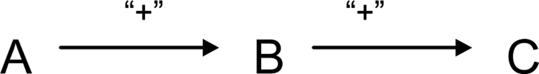
Example illustrating the informal use of positive and negative signs on edges

Suppose that the variables A and C are binary and B takes on values in the set {0, 1, 2}. Suppose further that pr(A = 1) = pr(A = 0) = 1/2, that the structural equations for B and C are as follows:

$$B=A+(1-A)*2{\epsilon }_{B}C=1(B=2)$$

where ε_B is Bernoulli with probability p < 1/2 and 1(B = 2) is the indicator function for B = 2. It follows that E[B_A=1] = 1 and E[B_A=0] = 2p < 1. Furthermore, E[C_B=0] = E[C_B=1] = 0 and E[C_B=2] = 1. Finally, we also have that E[C_A=0] = p and E[C_A=1] = 0. We thus have that increasing A increases B on average and increasing B increases C on average but in this example, intervening to increase A decreases C on average. Suppose that in a population of n individuals, p = 1/n then even though the departure from the requirements of a monotonic effect concerns only a single individual, intervening to increase A from 0 to 1 will still decrease C on average over the entire population.

We note that the lack of transitivity when signs are used to indicate average causal effects did not, in the example above, depend on the exact values of the distributions under consideration i.e. it arises for any p < 1/2. In fact, Wellman (1990) has shown that first order stochastic dominance (i.e. his qualitative influence) is the weakest possible relation between cumulative distribution functions for the transitivity of signs to hold.

4. Covariance and monotonic effects

The notions of monotonic effects and weak monotonic effects introduced above can be used to develop rules that govern monotonic effects and covariance. When the signs of directed paths relating two variables satisfy certain conditions, it is possible to determine the sign of the covariance of these variables. However, in order to prove the central result which provides these rules we need to make use of an additional probability lemma presented below. Lemma 5 is essentially a restatement of Theorem 2.1 in Esary et al. (1967).

Lemma 5

Let f and g be functions with n real-valued arguments such that both f and g are non-decreasing in each of their arguments. If X = (X₁, …, X_n) is a multivariate random variable with n components such that each component is independent of the other components then cov{f(X), g(X)} ≥ 0.

This probability lemma above allows us to prove Theorem 4 concerning the rules governing covariance and monotonic effects. Theorem 4 may be seen as a generalization of the corresponding result for recursive linear structural equation models which would follow quite simply from elementary path analysis (Duncan 1975).

Theorem 4

If A and Y are positively monotonically associated then Cov(A, Y) ≥ 0. If A and Y are negatively monotonically associated then Cov(A, Y) ≤ 0.

Theorem 4 concerns the sign of covariances. In related work (VanderWeele and Robins, 2007; VanderWeele and Robins, 2009b) we have derived rules governing the sign of conditional covariances in the presence of monotonic effects; however these rules require the development of theory concerning sufficient causation and assumptions beyond simply that of the presence of monotonic effects. If the directed paths relating two variables satisfy the conditions of Theorem 4, then this yields implications concerning the sign of the covariance of these variables. Obviously these conditions will not always hold; it will not always be possible to determine the sign of the covariance between any two variables simply from the signed causal directed acyclic graph. For a particular signed causal directed acyclic graph, Theorem 4 will yield implications concerning the signs of covariances for some pairs of variables and may fail to do so for others. Theorem 4 may fail to yield implications concerning the signs of covariances either because the signs of different directed paths are not congruent in the way required by the conditions of the theorem or because certain edges are without sign.

Example 3

Consider the signed directed acyclic graph given in Fig. 4 and note that no sign is present on the edge A → F.

Figure 4.

Example illustrating the relationship between covariance and monotonic effects

By Theorem 4, the covariance between B and C will be positive since the sign of the only directed path from B to C is positive and B and C have no common causes. The covariance between C and D will be negative since the sign of the only directed path from C to D is negative and because for the only common cause of C and D, namely A, all directed paths from A to C are positive and thus of the opposite sign as all directed paths from A to D not through C, which are negative. The covariance between E and F is undetermined because A is a common cause of E and F and the path from A to F consisting of the edge A → F is without sign. The covariance between D and E is also undetermined because the D → E edge is positive but A is a common cause of D and E and sign of the directed path A → B → C → D from A to D is negative and thus is of the opposite sign of the directed path from A to E consisting of the edge A → E which is positive.

As an additional application of Theorem 4, we return to the example given in the Introduction and illustrated by Figure 1 above, and we show that Theorem 4 can be used to draw conclusions about the presence of causal effects from the data even when data on confounding variables is missing.

Example 4

In Figure 1, recall that antihistamine treatment is denoted by E, asthma incidence by D, air pollution levels by A, and bronchial reactivity by C. Data is available only on antihistamine use E and asthma D. The effect of E on D is confounded by A and C. In this example it is arguably quite reasonable to assume that air pollution has a weak positive monotonic effect on bronchial reactivity, on antihistamine use (relative to bronchial reactivity C, the other parent of E) and on asthma (relative to relative to bronchial reactivity and antihistamine use). It is arguably also quite reasonable to assume that bronchial reactivity has a weak positive monotonic effect on antihistamine use (relative to air pollution) and on asthma (relative to air pollution and antihistamine use). We may then add to Figure 1 the positive signs indicated in Figure 5.

Figure 5.

Testing for the causal effect of E on D without data on A and C, using assumptions about signed edges

Suppose there were no causal effect of E on D so that the E → D edge were absent. There would then be no directed paths from E on D. Furthermore, if we consider every common cause of E and D, namely A and C, then we have that all directed paths from A to E are of the same sign as all directed paths from A to D and we also have that all directed paths from C to E are of the same sign as all directed paths from C to D. From Theorem 4 it would then follow that, if the E → D edge were absent, then Cov(E, D) ≥ 0. Suppose then we proceeded with an analysis of the association between E and D without data on A and C and suppose that we found that those using an antihistamine had lower asthma rates than those not using an antihistamine i.e. that Cov(E, D) < 0. We could then conclude that there was a causal effect of E on D, even though no data is available on A and C. This is because if E had no effect on D and if the monotonicity relationships indicated in Figure 5 held, then we would have Cov(E, D) ≥ 0. Note that the conclusions drawn here did not make any assumptions about the distributions of A, C, D and E beyond the monotonicity relationships.

5. Discussion

The extensions introduced in this paper provide the researcher with tools useful in drawing causal inferences. We have formalized the conditions under which signs can be added to the edges of a causal directed acyclic graph and have provided rigorous rules governing their use. We have also argued that a theory based only on average causal effects will be of limited use because it will not preserve transitivity. The result given in Theorem 3 governing the relationship between monotonic effects and causal effects in the presence of intermediate variables allows the researcher in certain cases to determine a priori whether a particular intervention will on average have a positive or negative effect. The rules governing monotonic effects and covariance given in Theorem 4 may assist the researcher in assessing whether assumptions being made about the causal structure of variables and about monotonic effects are in fact valid. We have also shown how Theorem 4 can be used to draw conclusions about the presence of causal effects even when certain confounding variables are not measured. The derivation of further results on assessing the sign of the bias that arises when particular signed backdoor paths are unblocked is a topic of current research and some preliminary results are available (VanderWeele et al., 2008). The directed acyclic graph causal framework has proved to be a useful tool in thinking carefully about questions of confounding and causal inference. It is hoped that these contributions will extend yet further the framework’s utilization and applicability.

Appendix A

A.1. Proof of theorem 1

Let P = {V₁, …, V_n} be an ordered list of the nodes on directed paths from A to B including A and B such that A = V₁ and B = V_n. Suppose that $W_1^n,\dots ,W_{t_n}^n$ are the parents of V_n in P such that the edges from $W_i^n$ to V_n are negative. Then the directed acyclic graph with $W_1^n,\dots ,W_{t_n}^n$ replaced by their negations has all edges from nodes in P into V_n positive. We prove the general result by proving inductively the following statement, which we denote by (*): For any k, there exists a set of nodes $W_1^k,\dots ,W_{t_k}^k$ in P such that if these nodes are replaced by their negations then all edges on all directed paths between any of the nodes V_k, …, V_n are positive and all edges from nodes in P into V_k, …, V_n are positive. Clearly this holds for k = n as shown above. We will show that if it holds for k = l then it holds also for k = l − 1. Let G′ be the graph with $W_1^l,\dots ,W_{t_l}^l$ replaced by their negations. Consider the parents of V_l−1 and let U₁, …, U_m be the parents of V_l−1 in P with negative edges into V_l−1. Let G″ be the graph G′ with U₁, …, U_m replaced by their negations. We will prove that G″ satisfies the properties required by (*) for k = l − 1; i.e. that taking $W_1^{l-1},\dots ,W_{t_{l-1}}^{l-1}=U_1,\dots ,U_m,W_1^l,\dots ,W_{t_l}^l$ satisfies (*) for k = l − 1. On G″, none of V_l, …, V_n can can be parents of V_l−1 so clearly all edges on all directed paths between any of the nodes V_l, …, V_n are positive. Furthermore, any edge from V_l−1 to one of V_l,…, V_n must be positive by virtue of (*) holding for k = l. Thus all edges on all directed paths between any of the nodes V_l−1, …, V_n are positive. Clearly all edges into V_l−1 are positive in G″. All edges into V_l, …, V_n were positive in G′ so the only possible way in which an edge into V_l, …, V_n in G″ could be negative is if it were an edge from one of U₁, …, U_m. Suppose there exist i, j such that the edge from the negation of U_i, −U_i, to V_j is negative in G″, where V_j is one of V_l, …, V_n. Then there exists a directed path from −U_i through V_l−1 to V_n that is positive and also a directed path from −U_i through V_j to V_n that is negative but this contradicts the hypothesis that the sign of all directed paths from A to B are positive. Thus none of U₁, …, U_m can be a parent of any of V_l, …, V_n and so all edges into V_l, …, V_n are positive in G″. Furthermore, it follows that U₁, …, U_m are distinct from $W_1^l,\dots ,W_{t_l}^l$ and that taking $W_1^{l-1},\dots ,W_{t_{l-1}}^{l-1}=U_1,\dots ,U_m,W_1^l,\dots ,W_{t_l}^l$ satisfies (*) for k = l − 1. The result follows.

A.2. Proof of theorem 2

We prove Theorem 2 in the case of weak monotonic effects. The case of monotonic effects is reasonably straightforward and follows by recursive substitution. By the properties of causal directed acyclic graphs, the original graph G can be marginalized to the causal directed acyclic graph H. Let C denote the set of common causes of A and Y. Let Q denote the set of nodes that are ancestors of A or of Y but are not descendents of A and not common causes of A and Y. By the corollary to Lemma 4 with X = {C,Q}, it follows that S(y|a, c, q) is non-decreasing in a and that the edge between A and Y is positive on H. Let Q₁ denote the subset of Q which are ancestors A; let Q₂ denote the subset of Q which are ancestors Y. As noted above, S(y|a, c, q) is non-decreasing in a. It remains to show that S(y|a, c) is non-decreasing in a. Because variables in Q₁ are ancestors of Y only through A we have that

$$S(y|a,c,q)=S(y|a,c,q_2).$$

Now variables in Q₂ are neither ancestors nor descendents of A; furthermore, C will contain all common cause of A and variables Q₂. From this it follows that A and Q₂ are d-separated given C. Thus

$$S(y|a,c)=E[S(y|a,c,Q_2)|a,c]=E[S(y|a,c,Q_2)|c]=E[S(y|a,c,Q)|c]$$

and since S(y|a, c,Q) is non-decreasing in a for all values of y, c, q we have that

$$S(y|a,c)=E[S(Y|a,c,Q)|c]$$

is non-decreasing in a.

A.3. Proof of theorem 3

Let C be the parents of A. By Lemma 4, E(Y|A = a, C = c) is non-decreasing in a for all values of c and by the back-door path criterion we have for a₁ ≥ a₂ that

$$E(Y_{A=a_1})={\sum }_{c}E(Y|A=a_1,C=c)P(C=c)\ge {\sum }_{c}E(Y|A=a_2,C=c)P(C=c)=E(Y_{A=a_2}).$$

A.4. Proof of theorem 4

We prove the result for positive monotonic association; the result for negative monotonic association follows by replacing the variable A with −A. We employ several times through this proof the result that

$$\mathit{\text{cov}}(Y,Z)=\mathit{\text{cov}}\{E(Y|X),E(Z|X)\}+E\{\mathit{\text{cov}}(Y,Z|X)\}.$$

By replacing each C_i with its negation if necessary we may assume that every path from C_i to A and from C_i to Y is of positive sign. Let C₁, …, C_n denote an ordered list of the nodes in C. Applying Theorem 1, we may replace certain nodes with their negations so that all edges on all directed paths from A to Y are positive. We may apply the algorithm in the proof of Theorem 1 to the directed paths from C_n to Y ignoring all the paths from C_n to Y through A so that by replacing certain variables with their negations all edges on all directed paths from C_n to Y not through A are of positive sign. We may apply the algorithm in the proof of Theorem 1 to the directed paths from C_n to A so that by replacing certain variables with their negations all edges on all directed paths from C_n to A are of positive sign. Note that the edges on directed paths from C_n to A cannot also be the edges on directed paths from C_n to Y not through A because by assumption C_n has no descendents that are common causes of A and Y. For C_i we may apply the algorithm in the proof of Theorem 1 first to directed paths from C_i to Y not through A, C_n, …, C_i+1 then to directed paths from C_i to A not through C_n, …, C_i+1, then from C_i to C_n not through C_n−1, …, C_i+1, then from C_i to C_j, j > i not through C_j−1, …, C_i+1 and finally from C_i to C_i+1. Applying this argument for each i we may replace certain variables with their negations so every edge on all directed paths from A to Y, from each C_i to A and from each C_i to Y is positive. By applying an argument similar to that in the proof of Theorem 2 the causal directed acyclic graph can be collapsed to one with only A and Y and their common causes C such that the edge between A and Y is positive and such that every edge on all directed paths from each C_i to A and from each C_i to Y is positive. We then have that

$$\mathit{\text{cov}}(A,Y)=\mathit{\text{cov}}\{E(A|C),E(Y|C)\}+E\{\mathit{\text{cov}}(A,Y|C)\}.$$

We will first show that E{cov(A, Y|C)} is non-negative. We have that

$$\mathit{\text{cov}}(A,Y|C)=E[\{A-E(A|C)\}\{Y-E(Y|C)\}|C]=E(E[\{A-E(A|C)\}\{Y-E(Y|C)\}|A,C]|C)=E[\{A-E(A|C)\}\{E(Y|A,C)-E(Y|C)\}|C]=\mathit{\text{cov}}\{A,E(Y|A,C)|C\}.$$

Given C, E(Y|A,C) is a non-decreasing function of A by the corollary of Lemma 4. Furthermore, given C, A is a non-decreasing function of A and thus by Lemma 5 we have that for each C, cov(A, Y|C) = cov{A, E(Y|A, C)|C} ≥ 0 and so

$$E\{\mathit{\text{cov}}(A,Y|C)\}\ge 0.$$

We will now show that cov{E(A|C), E(Y|C)} is non-negative. For each component C_i of C we may apply Lemma 4 in each case letting X be the non-descendents in C of C_i and letting R be the descendents in C of C_i. We then have that E(A|C) and E(Y|C) are non-decreasing in each component of C. Let f(C) = E(A|C) and g(C) = E(Y|C) so that cov{E(A|C), E(Y|C)} = cov{f(C), g(C)} where f(C) and g(C) are non-decreasing in each component of C. Let S₁ denote the subset of C which has no ancestors; let S₂ denote the subset of C which has no ancestors other than those in S₁; let S_i denote the subset of C which has no ancestors other than those in S₁, …, S_i−1 and let k be such that C = S₁, …, S_k. Note that given S₁, …, S_i−1 the components of S_i are independent of one another. We then have that

$$\mathit{\text{cov}}\{E(A|C),E(Y|C)\}=\mathit{\text{cov}}\{f(C),g(C)\}=\mathit{\text{cov}}[E\{f(C)|S_1\},E\{g(C)|S_1\}]+E[\mathit{\text{cov}}\{f(C),g(C)|S_1\}].$$

Applying the conditional covariance result again to the second of these two terms, conditioning on S₂ we have

$$\mathit{\text{cov}}\{f(C),g(C)\}=\mathit{\text{cov}}[E\{f(C)|S_1\},E\{g(C)|S_1\}]+E(\mathit{\text{cov}}[E\{f(C)|S_1,S_2\},E\{g(C)|S_1,S_2\}|S_1])+E[\mathit{\text{cov}}\{f(C),g(C)|S_1,S_2\}].$$

And continuing to iteratively apply the conditional covariance result to the final term gives

$$\mathit{\text{cov}}\{f(C),g(C)\}=\mathit{\text{cov}}[E\{f(C)|S_1\},E\{g(C)|S_1\}]+E(\mathit{\text{cov}}[E\{f(C)|S_1,S_2\},E\{g(C)|S_1,S_2\}|S_1])+E(\mathit{\text{cov}}[E\{f(C)|S_1,S_2,S_3\},E\{g(C)|S_1,S_2,S_3\}|S_1,S_2])+\dots +E(\mathit{\text{cov}}[E\{f(C)|S_1,\dots ,S_{k-1}\},E\{g(C)|S_1,\dots ,S_{k-1}\}|S_1,\dots ,S_{k-2}])+E[\mathit{\text{cov}}\{f(C),g(C)|s_1,\dots ,S_{k-1}\}].$$ (1)

Consider the ith term of this expression,

$$E(\mathit{\text{cov}}[E\{f(C)|S_1,\cdots ,S_i\},E\{g(c)|S_1,\dots ,S_i\}|S_1,\dots ,S_{i-1}]).$$

Now

$$E\{f(C)|S_1,\dots ,S_i\}=E[E[\dots E[E\{f(C)|S_1,\dots ,S_{k-1}\}|S_1,\dots ,S_{k-2}]|\dots |S_1,\dots ,S_{i+1}]|S_1,\dots ,S_i].$$

Let $S_k^1,\dots ,S_k^{n_k}$ be any ordering of the elements S_k. We have that f(C) is non-decreasing in S₁, …, S_k−1 and S_k. Furthermore, for the jth component $S_k^j$ of S_k we have that $S(s_k^j|s_1,\dots ,s_{k-1},s_k^1,\dots ,s_k^{j-1})=S(s_k^j|s_1,\dots ,s_{k-1})$ is non-decreasing in s₁, …, s_k−1 since all edges from S₁, …, S_k−1 to S_k are of positive sign and so by repeated application of Lemma 3 we have that E{f(C)|S₁, …, S_k−1} is non-decreasing in S₁, …, S_k−1. Similarly if $S_{k-1}^1,\dots ,S_{k-1}^{n_{k-1}}$ is any ordering of the elements S_k−1 then for the jth component $S_{k-1}^j$ we have that $S(s_{k-1}^j|s_1,\dots ,s_{k-2},s_{k-1}^1,\dots ,s_{k-1}^{j-1})=S(s_{k-1}^j|s_1,\dots ,s_{k-2})$ is non-decreasing in s₁, …, s_k−2 and so by repeated application of Lemma 3 we have that E[E{f(C)|S₁, …, S_k−1}|S₁, …, S_k−2] is non-decreasing in S₁, …, S_k−2. Carrying the argument forward we have that

$$E\{f(C)|S_1,\dots ,S_i\}=E[E[\dots E[E\{f(C)|S_1,\dots ,S_{k-1}\}|S_1,\dots ,S_{k-2}]|\dots |S_1,\dots ,S_{i+1}]|S_1,\dots ,S_i]$$

is non-decreasing in S₁, …, S_i. Similarly E{g(C)|S₁, …, S_i}is non-decreasing in S₁, …, S_i and so conditional on S₁, …, S_i−1, E{f(C)|S₁, …, S_i} and E{g(C)|S₁, …, S_i} are both non-decreasing functions of the independent random variables S_i and thus by Lemma 5,

$$\mathit{\text{cov}}[E\{f(C)|S_1,\dots ,S_i\},E\{g(C)|S_1,\dots ,S_i\}|S_1,\dots ,S_{i-1}]\ge 0$$

and so

$$E(\mathit{\text{cov}}[E\{f(C)|S_1,\dots ,S_i\},E\{g(C)|S_1,\dots ,S_i\}|S_1,\dots ,S_{i-1}])\ge 0.$$

Since each term of (1) is non-negative we have that

$$\mathit{\text{cov}}\{E(A|C),E(Y|C)\}=\mathit{\text{cov}}\{f(C),g(C)\}\ge 0.$$

This completes the proof.

References

- Archer NP, Wang S. Application of the backpropagation neural network algorithm with monotonicity constraints for two-group classification problems. Decision Sciences. 1993;24:60–75. [Google Scholar]
- Bioch JC. Dualization, decision lists and identification of monotone discrete functions. Annals of Mathematics and Artificial Intelligence. 1998;13:69–91. [Google Scholar]
- Brumback BA, Hernán MA, Haneuse SJPA, Robins JM. Sensitivity analyses for unmeasured confounding assuming a marginal structural model for repeated measures. Statist. Med. 2004;23:749–767. doi: 10.1002/sim.1657. [DOI] [PubMed] [Google Scholar]
- Cox DR, Wermuth N. A general condition for avoiding effect reversal after marginalization. J. R. Statist. Soc. B. 2003;65:937–941. [Google Scholar]
- Dawid AP. Causal inference without counterfactuals. J. Am. Statist. Assoc. 2000;95:407–424. [Google Scholar]
- Dawid AP. Influence diagrams for causal modelling and inference. Int. Statist. Rev. 2002;70:161–189. [Google Scholar]
- Druzdzel MJ, Henrion M. Proceedings of the 11th Annual Conference on Artificial Intelligence. Washington, D.C.: 1993. Efficient reasoning in qualitative probabilistic networks; pp. 548–553. [Google Scholar]
- Duncan OD. Introduction to Structural Equation Models. New York: Academic Press; 1975. [Google Scholar]
- Esary JD, Proschan F, Walkup DW. Association of random variables, with applications. Ann. Math. Statist. 1967;38:1466–1474. [Google Scholar]
- Galles D, Pearl J. Testing identifiability of causal effects. In: Besnard P, Hanks S, editors. Uncertainty in Artificial Intelligence. Vol. 11. San Francisco: Morgan Kaufman; 1995. pp. 185–195. [Google Scholar]
- Geiger D, Verma TS, Pearl J. Identifying independence in bayesian networks. Networks. 1990;20:507–534. [Google Scholar]
- Geng Z, Guo J, Fung WK. Criteria for confounders in epidemiological studies. J. R. Statist. Soc. B. 2002;64:3–15. [Google Scholar]
- Greenland S, Pearl J, Robins JM. Causal diagrams for epidemiologic research. Epidemiology. 1999;10:37–48. [PubMed] [Google Scholar]
- Haavelmo T. The statistical implications of a system of simultaneous equations. Econometrica. 1943;11:1–12. [Google Scholar]
- Kuroki M, Miyakawa M. Identifiability criteria for causal effects of joint interventions. J. Jap. Statist. Soc. 1999;29:105–117. [Google Scholar]
- Kuroki M, Miyakawa M. Covariate selection for estimating the causal effect of control plans using causal diagrams. J. R. Statist. Soc. B. 2003;65:209–222. [Google Scholar]
- Lauritzen SL, Dawid AP, Larsen BN, Leimer HG. Independence properties of directed Markov fields. Networks. 1990;20:491–505. [Google Scholar]
- Lauritzen SL, Richardson TS. Chain graph models and their causal interpretations (with discussion) J. Roy. Statist. Soc. Ser. B. 2002;64:321–361. [Google Scholar]
- Lin DY, Psaty BM, Kronmal RA. Assessing the sensitivity of regression results to unmeasured confounding in observational studies. Biometrics. 1998;54:948–963. [PubMed] [Google Scholar]
- Manski CF. Monotone treatment response. Econometrica. 1997;65:1311–1334. [Google Scholar]
- Pearl J. Comment: Graphical models, causality, and intervention. Statist. Sci. 1993;8:266–269. [Google Scholar]
- Pearl J. Causal diagrams for empirical research. Biometrika. 1995;82:669–688. [Google Scholar]
- Pearl J. Causality: Models, Reasoning, and Inference. Cambridge: Cambridge University Press; 2000. [Google Scholar]
- Pearl J, Robins JM. Probabilistic evaluation of sequential plans from causal models with hidden variables. In: Besnard P, Hanks S, editors. Uncertainty in Artificial Intelligence. Vol. 11. San Francisco: Morgan Kaufman; 1995. pp. 444–453. [Google Scholar]
- Potharst R, Feelders A. Classification trees for problems with monotonicity constraints. Special Interest Group on Knowledge Discovery and Data Mining Explorations. 2002;4:1–10. [Google Scholar]
- Robins JM. A new approach to causal inference in mortality studies with sustained exposure period - application to control of the healthy worker survivor effect. Mathematical Modelling. 1986;7:1393–1512. [Google Scholar]
- Robins JM. Addendum to a new approach to causal inference in mortality studies with sustained exposure period - application to control of the healthy worker survivor effect. Computers and Mathematics with Applications. 1987;14:923–945. [Google Scholar]
- Robins JM. Discussion of "Causal diagrams for empirical research". In: Pearl J, editor. Biometrika. Vol. 82. 1995. pp. 695–698. [Google Scholar]
- Robins JM. Causal inference from complex longitudinal data. In: Berkane M, editor. Latent Variable Modeling and Applications to Causality. Vol. 120. New York: Springer Verlag; 1997. pp. 69–117. Lecture Notes in Statistics. [Google Scholar]
- Robins JM. Semantics of causal DAG models and the identification of direct and indirect effects. In: Green P, Hjort NL, Richardson S, editors. Highly Structured Stochastic Systems. New York: Oxford University Press; 2003. pp. 70–81. [Google Scholar]
- Rosenbaum PR, Rubin DB. The central role of the propensity score in observational studies for causal effects. Biometrika. 1983a;70:41–55. [Google Scholar]
- Rosenbaum PR, Rubin DB. Assessing sensitivity to an unobserved binary covariate in an observational study with binary outcome. J. R. Statist. Soc. B. 1983b;45:212–218. [Google Scholar]
- Spirtes P, Glymour C, Scheines R. Causation, Prediction and Search. New York: Springer-Verlag; 1993. [Google Scholar]
- Tian J, Pearl J. Proceedings of the Eighteenth National Conference on Artificial Intelligence. Menlo Park: AAAI Press/The MIT Press; 2002. On the identification of causal effects; pp. 567–573. [Google Scholar]
- van der Gaag LC, Bodlaender HL, Feelders A. Monotonicity in Bayesian networks. In: Chickering M, Halpern J, editors. Uncertainty in Artificial Intelligence. Vol. 20. San Francisco: Morgan Kaufman; Menlo Park: AAAI Press/The MIT Press; 2004. pp. 569–576. [Google Scholar]
- VanderWeele TJ, Hernán MA, Robins JM. Causal directed acyclic graphs and the direction of unmeasured confounding bias. Epidemiology. 2008;19:720–728. doi: 10.1097/EDE.0b013e3181810e29. [DOI] [PMC free article] [PubMed] [Google Scholar]
- VanderWeele TJ, Robins JM. Directed acyclic graphs, sufficient causes and the properties of conditioning on a common effect. Am. J. Epidemiol. 2007;166:1096–1104. doi: 10.1093/aje/kwm179. [DOI] [PubMed] [Google Scholar]
- VanderWeele TJ, Robins JM. Properties of monotonic effects on directed acyclic graphs. Journal of Machine Learning Research. 2009a;10:699–718. [Google Scholar]
- VanderWeele TJ, Robins JM. Minimal sufficient causation and directed acyclic graphs. Annals of Statistics. 2009b;37:1437–1465. [Google Scholar]
- Verma T, Pearl J. Causal networks: Semantics and expressiveness. In: Shachter R, Levitt TS, Kanal LN, editors. Proceedings of the 4th Workshop on Uncertainty in Artificial Intelligence. Vol. 4. Amsterdam: Elesevier; 1988. pp. 69–76. 352–359. Reprinted in Uncertainty in Artificial Intelligence. [Google Scholar]
- Wellman MP. Fundamental concepts of qualitative probabilistic networks. Artificial Intelligence. 1990;44:257–303. [Google Scholar]
- Wright S. Correlation and causation. J. Agric. Res. 1921;20:557–585. [Google Scholar]