

Abstract
The frontal eye field (FEF) plays a central role in saccade selection and execution. Using artificial stimuli, many studies have shown that the activity of neurons in the FEF is affected by both visually salient stimuli in a neuron's receptive field and upcoming saccades in a certain direction. However, the extent to which visual and motor information is represented in the FEF in the context of the cluttered natural scenes we encounter during everyday life has not been explored. Here, we model the activities of neurons in the FEF, recorded while monkeys were searching natural scenes, using both visual and saccade information. We compare the contribution of bottom-up visual saliency (based on low-level features such as brightness, orientation, and color) and saccade direction. We find that, while saliency is correlated with the activities of some neurons, this relationship is ultimately driven by activities related to movement. Although bottom-up visual saliency contributes to the choice of saccade targets, it does not appear that FEF neurons actively encode the kind of saliency posited by popular saliency map theories. Instead, our results emphasize the FEF's role in the stages of saccade planning directly related to movement generation.
Keywords: attention, fixation choice, generalized linear models, natural stimuli, neural data analysis, visuomotor integration
Introduction
One of the most frequent decisions in our lives is where to look next. How the nervous system makes this decision while free-viewing or searching for a target in natural scenes is an ongoing topic of research in computational neuroscience (Yarbus 1967; Koch and Ullman 1985; Kayser et al. 2006; Elazary and Itti 2008; Ehinger et al. 2009; Foulsham et al. 2011; Zhao and Koch 2011). The most prominent models of saccade target selection during free-viewing are based on the concept of bottom-up saliency maps. In these models, the image is separated into several channels including color, light intensity, and orientation, to create a set of “feature maps” (for a review, see Koch and Ullman 1985; Treisman 1988; Cave and Wolfe 1990; Schall and Thompson 1999; Itti and Koch 2000, 2001). For example, the horizontal feature map would have high values wherever the image has strong horizontal edges. After normalizing and combining these feature maps, the output indicates locations in an image containing features that are different from the rest of the image. The more dissimilar an image region is from the rest of the image the more salient or “surprising” it is (Itti and Baldi 2006). Saliency models for saccade target-selection predict that human subjects are more likely to look at locations that are salient in the sense of being different from the rest of the image. Models based on these ideas have successfully described eye-movement behavior in both humans and monkeys (Einhäuser et al. 2006; Berg et al. 2009; Foulsham et al. 2011). How the brain may implement such algorithms is a central question in eye-movement research.
The involvement of cerebral cortex in this selection of eye movements has been recognized since the late 19th century when David Ferrier reported that eye-movements could be evoked from several regions of the rhesus monkey's cerebral cortex by using electrical stimuli (Ferrier 1875). One of these regions included an area of cortex now known as the frontal eye field (FEF). The visual and movement-related response field properties of different classes of neurons in the FEF have been carefully characterized using physiological and behavioral methods (Bizzi 1968; Bizzi and Schiller 1970; Mohler et al. 1973; Suzuki and Azuma 1977; Schiller et al. 1980; Bruce and Goldberg 1985; Segraves and Goldberg 1987; Schall 1991; Segraves 1992; Schall and Hanes 1993; Segraves and Park 1993; Burman and Segraves 1994; Dias et al. 1995; Schall et al. 1995; Bichot et al. 1996; Sommer and Tehovnik 1997; Dias and Segraves 1999; Everling and Munoz 2000; Sommer and Wurtz 2001; Sato and Schall 2003; Thompson and Bichot 2005; Fecteau and Munoz 2006; Serences and Yantis 2006; Ray et al. 2009; Phillips and Segraves 2010). In addition to eye-movement related activity, FEF firing rates are thought to be affected by simple image features (Peng et al. 2008), by task-relevant features (Thompson et al. 1996, 1997; Bichot and Schall 1999; Murthy et al. 2001), and by higher-order cognitive factors including memory and expectation (Thompson et al. 2005). During the period of fixation between saccades, the initial visual activity of FEF neurons is not selective for specific features such as color, shape, or direction of motion (Schall and Hanes 1993). Later activity, however, is more closely related to saccade target selection, and appears to be influenced by both the intrinsic, bottom-up saliency of potential targets as well by their similarity to the target (Murthy et al. 2001; Thompson and Bichot 2005; Thompson et al. 2005). Several studies have suggested that the pre-saccadic peak of FEF visual activity specifies the saccade target (Schall and Hanes 1993; Schall et al. 1995; Bichot and Schall 1999) and that this visual selection signal is independent of saccade production (Thompson et al. 1997; Murthy et al. 2001; Sato et al. 2001; O'Shea et al. 2004). In summary, activity in FEF has been linked to information about perception, decision making, planning, and action, increasing the difficulty of identifying a precise computational role for this area.
Although it has been suggested that FEF neurons encode a visual saliency map, the definition for visual saliency in this context is typically largely subjective, nonuniform across studies, not always explicitly defined, and based primarily upon the likelihood that a feature in visual space will become the target for a saccade (Thompson and Bichot 2005). From a computational perspective, the prevalent interpretation of saliency in the oculomotor field includes the fundamental visual features contributing to the objective definition of visual saliency as well as other factors determining saccade target choice including relevance or similarity to the search target and the gist—the likelihood that the target will be found at a particular location (Itti and Koch 2000; Land and Hayhoe 2001; Oliva et al. 2003; Turano et al. 2003). In this study, we use a precise bottom-up definition of saliency, a definition that is independent of task objective or gist, based only upon the basic physical image features. Examining FEF activity in the light of a formal definition will advance our understanding of both the process for saccade target choice as well as the role of the FEF in that process.
It is unclear whether results from earlier studies using artificial stimuli will hold for natural scenes, and exactly how visual and motor information are represented in FEF during naturalistic eye movements. To understand how the brain works ultimately implies understanding how it solves the kinds of tasks encountered during everyday life (Kayser et al. 2004). Following that philosophy, multiple communities have begun to analyze the brain using natural stimuli (Rolls and Tovee 1995; Willmore et al. 2000; Theunissen et al. 2001; Vinje and Gallant 2002; Wainwright et al. 2002; Smyth et al. 2003; Weliky et al. 2003; Sharpee et al. 2004) and have quantified the statistics of natural scenes and movements (Olshausen and Field 1996; Bell and Sejnowski 1997; Van Hateren and van der Schaaf 1998; Schwartz and Simoncelli 2001; Lewicki 2002; Hyvarinen et al. 2003; Srivastava et al. 2003; Betsch et al. 2004; Smith and Lewicki 2006; Ingram et al. 2008; Howard et al. 2009). Importantly, these studies show experimentally that surprising nonlinear aspects of processing become apparent as soon as natural stimuli are used (Theunissen et al. 2000; Kayser et al. 2003; MacEvoy et al. 2008). For example, input to regions outside of the classical receptive field during natural scene viewing increases the selectivity and information transfer of V1 neurons (Vinje and Gallant 2002). It is thus important to analyze FEF activity using natural stimuli.
Although a complete understanding of the FEF's role in eye movement control will depend on the use of natural stimuli, analyzing neural activities during the search of natural images is a difficult problem. The main factor contributing to this difficulty is the fact that most variables of interest are correlated with one another. It is known that monkeys tend to look at visually salient regions of images (Einhäuser et al. 2006; Berg et al. 2009). This means that a purely movement-related neuron would have correlations with bottom-up saliency. In an extreme example, eye muscle motor neurons responsible for moving the eyes to the right, would on average have more activity during times where the right side of the image has high saliency, and would thus appear to encode high saliency in the right visual field. We clearly would not want to conclude that the motor neuron encodes saliency. This emphasizes the need for a way of dealing with the existing correlations.
To deal with such cases, statistical methods have been developed that enable “explaining away” (Pearl 1988). In natural scene search, the correlations are not perfect—the subject may not always look to the right when the rightward region is salient. These divergences enable us to identify the relative contributions of visual and motor activation to neuron spiking. The basic intuition is the following: For the case of a neuron that is tuned only to saliency, its activity may also be correlated with eye movement direction due to the imperfect correlation of saliency and saccade direction during natural scene search. Once we subtract the best prediction based on saliency, however, any correlation with movement would be gone. The opposite would not be true. If we subtract the best prediction based on movement, a correlation with saliency would still exist. Over the past few years, generalized linear models (GLMs), have proven to be powerful tools for solving such problems, modeling spike trains when neural activity may depend on multiple, potentially correlated, variables (Truccolo et al. 2005; Pillow et al. 2008; Saleh et al. 2010).
Here, we recorded from neurons in the FEF while a monkey searched for a small target embedded in natural scenes. We then analyzed the spiking activity of these neurons using GLMs that treat both bottom-up saliency and saccades as regression variables. Almost all neurons had correlations with upcoming saccades and most also had correlations with bottom-up saliency. However, after taking into account the saccade-related activities, the correlations with saliency were explained away. These results suggest that conventional, bottom-up saliency is not actively encoded in the FEF during natural scene search.
Materials and Methods
The animal surgery, training, and neurophysiological procedures used in these experiments are identical to those reported in (Phillips and Segraves 2010). All procedures for training, surgery, and experiments were approved by Northwestern University's Animal Care and Use Committee.
Animals and Surgery
Two female adult rhesus monkeys (Macaca mulatta) were used for these experiments, identified here as MAS14 and MAS15. Each monkey received preoperative training followed by an aseptic surgery to implant a subconjunctival wire search coil for recording eye movements (Robinson 1963; Judge et al. 1980), a Cilux plastic recording cylinder aimed at the FEF, and a titanium receptacle to allow the head to be held stationary during behavioral and neuronal recordings. Surgical anesthesia was induced with the short-acting barbituate thiopental (5–7 mg/kg IV), and maintained using isoflurane (1.0%–2.5%) inhaled through an endotracheal tube. The FEF cylinder was centered at stereotaxic coordinates anterior 25 mm and lateral 20 mm. The location of the arcuate sulcus was then visualized through the exposed dura and the orientation of the cylinder adjusted to allow penetrations that were roughly parallel to the bank of the arcuate sulcus. Both monkeys had an initial cylinder placed over the left FEF. Monkey MAS14 later had a second cylinder place over the right FEF.
Behavioral Paradigms
We used the REX system (Hays et al. 1982) based on a PC computer running QNX (QNX Software Systems, Ottawa, Ontario, Ca), a real-time UNIX operating system, for behavioral control and eye position monitoring. Visual stimuli were generated by a second, independent graphics process (QNX – Photon) running on the same PC and rear-projected onto a tangent screen in front of the monkey by a CRT video projector (Sony VPH-D50, 75 Hz noninterlaced vertical scan rate, 1024 × 768 resolution). The distance between the front of the monkey's eye to the screen was 109.22 cm (43 inches).
Visually Guided and Memory-Guided Delayed Saccade Tasks
Monkeys fixated a central red dot for a period of 500–1000 ms. At the end of this period, a target stimulus appeared at a peripheral location. On visually guided trials, the target remained visible for the duration of the trial. On memory-guided trials, the target disappeared after 350 ms. After the onset of the target, monkeys were required to maintain central fixation for an additional 700–1000 ms until the central red dot disappeared, signaling the monkey to make a single saccade to the target (visually guided) or the location at which the target had appeared (memory-guided). The delay period refers to the period of time between the target onset and the disappearance of the fixation spot. These 2 tasks were used to characterize the FEF cells by comparing neural activity during 4 critical epochs (see Data Analysis section). Typically, trials of these types were interleaved with each other, and with the scene search tasks described below.
Scene Search Task
This task was designed to generate large numbers of purposeful, self-guided, saccades. Monkeys were trained to find a picture of a small fly embedded in photographs of natural scenes. After monkeys learned the standard visually guided and memory-guided search tasks, the target spot was replaced with the image of the fly. After 30 min, the scene task was introduced. Both monkeys used in this experiment immediately and successfully sought out the fly. After a few sessions performing this task, it became obvious that monkeys were finding the target after only 1 or 2 saccades. We therefore used a standard alpha blending technique to superimpose the target onto the scene. This method allows for varying the proportions of the source (target) and destination (the background scene) for each pixel, and was used to create a semi-transparent target. Even after extensive training, we found that the task was reasonably difficult with a 65% transparent target, requiring the production of multiple saccades while the monkeys searched for the target. Monkeys began each trial by fixating a central red dot for 500–1000 ms, then the scene and embedded target appeared simultaneously with the disappearance of the fixation spot, allowing monkeys to begin searching immediately. The fly was placed pseudo randomly such that its appearance in 1 of 8 45° sectors of the screen was balanced. Within each sector its placement was random between 3° and 30° of visual angle from the center of the screen. Trials ended when the monkeys fixated the target for 300 ms, or failed to find the target within 25 saccades. Images of natural scenes were pseudorandomly chosen from a library of >500 images, such that individual images were repeated only after all images were displayed. An essential feature of this task is that, although they searched for a predefined target, the monkeys themselves decided where to look. The location where the target was placed on the image did not predict the amplitudes and directions of the saccades that would be made while searching for it nor the vector of the final saccade that captured it.
Image Database
The set of images was collected by one of the co-authors (ANP) for the purpose of conducting the experiment in Phillips and Segraves (2010), and is available for download. The photographs were taken using a digital camera, and included scenes with engaging objects such as animals, people, plants, or food. The images were taken by a human photographer and thus may contain biases not present in truly natural visual stimuli (Tseng et al. 2009). For instance, the center of the image tends to be more salient than the edges (as presented in Results section, Fig. 2A,B).
Figure 2.
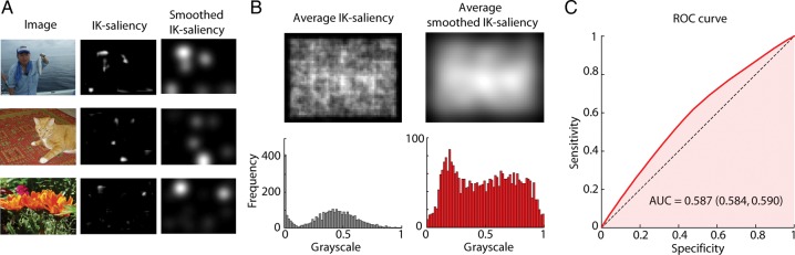
Saliency maps and saccade prediction. (A) Three typical images from the natural scene search task, along with their IK-saliency maps, and smoothed IK-saliency maps (filtered with an isotropic Gaussian with a standard deviation of 5°). (B) (top) Average IK-saliency map across all images used in the task along with the average smoothed IK-saliency. Note that there is a bias towards the center of the image being more salient than the edges. (bottom) Corresponding image histograms. (C) ROC curve for smoothed IK-saliency as an eye fixation predictor. We considered all the saccades for both monkeys in the interval between 200 and 2000 ms of each trial. Area under the curve (median and 95% confidence interval, boostrap) is shown.
Neural Recording
Single neuron activity was recorded using tungsten microelectrodes (A-M Systems, Inc., Carlsborg, WA, USA). Electrode penetrations were made through stainless steel guide tubes that just pierced the dura. Guide tubes were positioned using a Crist grid system (Crist et al. 1988, Crist Instrument, Co., Hagerstown, MD, USA). Recordings were made using a single electrode advanced by a hydraulic microdrive (Narashige Scientific Instrument Lab, Tokyo, Japan). On-line spike discrimination and the generation of pulses marking action potentials were accomplished using a multichannel spike acquisition system (Plexon, Inc., Dallas, TX, USA). This system isolated a maximum of 2 neuron waveforms from a single FEF electrode. Pulses marking the time of isolated spikes were transferred to and stored by the REX system. During the experiment, a real-time display generated by the REX system showed the timing of spike pulses in relationship to selected behavioral events.
The location of the FEF was confirmed by our ability to evoke low-threshold saccades from the recording sites with current intensities of ≤50 μA, and the match of recorded activity to established cell activity types (Bruce and Goldberg 1985). To stimulate electrically, we generated 70 ms trains of biphasic pulses, negative first, 0.2 ms width per pulse phase delivered at a frequency of 330 Hz.
Data Analysis – General Analysis
FEF Cell Characterization
We examined average cell activity during 4 critical epochs while the monkey performed the memory-guided delayed saccade task to determine if the cell displayed visual or premotor activity. If not enough data were available from this task, data from the visually guided delayed saccade task was used. The baseline epoch was the 200 ms preceding target onset, the visual epoch was 50–200 ms after target onset, the delay epoch was the 150 ms preceding the disappearance of the fixation spot, and the presaccade epoch was the 50 ms preceding the saccade onset. FEF cells were characterized by comparing epochs in the following manner using the Wilcoxon sign-rank test. If average firing rates during the visual or delay epochs was significantly higher than the baseline rate, the cell was considered to have visual or delay activity respectively. If the activity during the presaccade epoch was significantly greater than the delay epoch, the cell was considered to have premotor activity. These criteria are similar to those used by Sommer and Wurtz (2000). The selection of neurons for this study was biased towards those with visual activity and our sample does not include any neurons with only motor activity.
IK-Saliency
We considered the Itti-Koch (IK)-saliency (Itti and Koch 2000; Walther and Koch 2006) as the definition of saliency (see Supplementary Material and Supplementary Fig. S1A). This method provides a bottom-up definition of saliency based only on basic image features and independent of task objectives. We used the publicly available toolbox (Walther and Koch 2006) for computing IK-saliency with the default parameter values and considered 3, equally weighted, channels: color, intensity and orientation. IK-saliency for each image was centered by subtracting the mean of the IK-saliency of that image. To account for a possible imprecision of eye position tracking, we low-pass filtered the IK-saliency using a 5° standard deviation 2D-Gaussian (some examples are shown in Results section, Fig. 2A). We redid the analysis either without centering or without low-pass filtering the definition of IK-saliency and show that the conclusions of this study are the same (these results are shown in Supplementary Material, Supplementary Fig. S5).
ROC Curve
To compute the Receiver Operator Characteristic (ROC) curve for IK-saliency as an eye fixation predictor we considered all the saccades for both monkeys in the interval between 200 and 2000 ms of each trial. We varied a threshold across the domain of possible values of IK-saliency and determined the fraction of fixations that fell on pixels with IK-saliency above that threshold (y-axis of ROC curve). We compared this true positive rate across all frames to the fraction of pixels without fixations that had IK-saliency above the threshold (the false positive rate). We bootstrapped across the pixels with fixations to obtain a 95% confidence interval for the area under the ROC curve.
Finally, to test for the predictive value of saliency independent of center-bias, we compared, using Mann-Whitney test, the IK-saliency at the fixated locations with the IK-saliency at the same locations in all other images.
Peri/Post-Stimulus Time Histograms (PSTHs)
We used PSTHs to examine preferred directions for saccades as well as sensitivity to visual saliency. For the saccade-related PSTHs, we considered a time interval of 400 ms centered on saccade onset. We considered all saccades in the time period of 200 ms after trial start and until a maximum of 5000 ms into the trial (less if the trial ended before 5000 ms). We assigned the neuron's activity for each 400 ms perisaccadic interval to one of 8 PSTHs according to the saccade direction and ignoring the magnitude of the saccade. To construct the PSTHs, spikes were binned in 10 ms windows and averaged across trials.
The PSTHs for activity driven by visual saliency were computed in an analogous way. Each of our analyses considers the whole distribution of IK-saliency over the scene to characterize neural responses. We considered a time interval of 400 ms centered on fixation onset. The spikes were binned in 10 ms windows. Activity for a fixation interval was assigned to a particular direction if, after convolving the IK-saliency image with one of 8 filter windows that corresponded to each representative direction relative to eye fixation, the average pixel value was positive. Unlike the saccade-related PSTHs where each raster was associated with only one of the 8 representative directions, IK-saliency for a given image was often elevated in more than one of the 8 filter windows, and thus each raster in the visual saliency PSTHs could be assigned to more than one PSTH. The 8 filter windows were cosine functions of the angle, each with a maximum at the correspondent representative direction and independent of the distance to fixation point. These filters were thresholded to be zero at a distance smaller than 3° or larger than 60°.
Data Analysis – Generative Model, Model Fitting and Model Comparison
To explicitly model the joint contribution of saliency and saccades we developed a generative model for FEF spiking using a type of GLM—a linear–nonlinear-Poisson cascade model. We specify how these multiple variables can affect neural firing rates and how firing rates translate to observed spikes. We then fit the model to the observed spikes using maximum likelihood estimation (see below).
Generative Model
We considered a time interval starting 200 ms after trial start and until a maximum of 5000 ms into the trial. We wanted to examine 3 hypotheses: spike trains in FEF neurons encode 1) saccade-related (motor) information alone, 2) bottom-up saliency alone, or 3) both motor processes and bottom-up saliency. We model spike activity using a Generalized Bilinear Model (Ahrens et al. 2008). We will explain in detail the joint model, that is, the model that considers both saccade and saliency as covariates—candidate predictors of FEF neuron activity. The saccade only, saliency only and full-saccade models are simplifications of this basic model and will be described after. We start by assuming that the conditional intensity (instantaneous firing rate), , of a neuron at time is a function of the eye movements , visual stimuli, , as well as the time relative to saccade onsets, , and time relative to fixation onsets, :
| (1) |
We assume that there are 2 spatiotemporal receptive fields (STRFs) and for motor (saccade) and for visual (saliency) covariates, respectively. To account for possible nonspatially tuned responses (e.g., untuned temporal modulation preceding fixation onset in a saliency encoding neuron or saccade-locked untuned firing rate change) and for the fact that saccades do not have a fixed duration (a histogram of saccade durations is shown in Supplementary Fig. S2B), we also allow for the possibility of a purely temporal response—independent of direction of saccade or of saliency stimuli—defined by temporal receptive fields (TRFs) at beginning of saccade, and at end of saccade/beginning of fixation, We assume that these STRFs and TRFs combine linearly and, to ensure that the firing rate is positive, the output of this linear combination is then passed through an exponential nonlinearity. To simplify, we assume that the STRFs are space-time separable:
| (2) |
and that both the TRFs and the STRFs are linear in some basis, such that they can be rewritten as a sum of linear and bilinear forms,
| (3) |
The vectors and define the temporal components of the STRFs, while and define the respective spatial components. The parameter defines the baseline intensity and and are the parameters for the purely temporal responses centered at saccade and fixation onset, respectively. These parameters, together with the motor parameters and , as well as the saliency parameters and of the STRF, fully define the neurons firing rate. Notice that the bilinear components of the model are not strictly linear in the parameters unless we consider the temporal components and the spatial components separately.
Finally, we assume that the observed spikes are drawn from a Poisson random variable with this rate:
| (4) |
Hence if is the number of spikes during the interval ,
We binned the data in intervals and we assume constant firing rate within each time bin, hence
For notational convenience, in the remainder of the Methods will denote an index representing the time bin , with .
Parametrization of the Receptive Fields
The form of the STRFs depends on how we construct and , that is, how we parameterize the spatial and temporal components of the saccade and saliency receptive fields. We parameterize the spatial receptive field for saccades by assuming that the activity of the neuron is cosine tuned for saccade direction, i.e., its firing rate is a function of the cosine of the angular difference between the direction of saccade and some fixed direction, the neuron's preferred direction (Georgopoulos et al. 1982; Hatsopoulos et al. 2007). Specifically, for each time index , we define a vector as:
| (5) |
if a saccade with direction occurred at time index , otherwise . For notation convenience, we define a matrix , where . This matrix incorporates the spatial component of the saccade covariates for each of the spatial basis functions for all time points. Although there is some evidence that FEF neurons may be tuned to saccade magnitude (Bruce and Goldberg 1985), we focus on directional tuning here, which appears to be the dominant factor. The construction of and , which defines the form of the TRFs, is done in an analogous way by defining vector as (1D) if a saccade occurred at time index and otherwise. To model temporal variation near the time of saccade and fixation onset, we parameterized TRFs with a set of 5 basis functions. As saccades and fixations are defined by very specific points in time, we restrict ourselves to finite windows 200 ms before to 300 ms after saccade or fixation onset. Specifically, our set of temporal basis functions are 5 truncated Gaussians with standard deviation of 50 ms:
| (6) |
where is the indicator function, and the means are equally spaced such that they partition the interval between −200 and 300 ms into 6 subintervals: ms with . We incorporate temporal information by convolving each column of matrix with each basis function that parameterizes the TRFs. Finally, we define, for each time index , the matrix where
| (7) |
The matrix is defined in an analogous way and is hence a 5-by-1 matrix.
For the visual/saliency basis we assume a similar model where the neuron has a preferred direction for the saliency surrounding the eye fixation position. This model is based on the entire saliency distribution across the scene. The parameterization is analogous to the saccade spatial receptive field:
| (8) |
if a fixation started at time and otherwise. denotes the IK-saliency of the current image and the sum is over all pixel positions in a window centered at the eye position during fixation (see Supplementary Material and the description above and (Itti and Koch 2000; Walther and Koch 2006) for details). Similar to the cosine tuning to saccade direction used above, this representation provides a directional tuning to average saliency. We considered the median eye position during the fixation period as the value of eye position during the ith fixation, . The construction of matrices and is then analogous to the construction of and .
The STRFs for saccades and saliency allow us to model directional dependence that is then modulated by an envelope around the time of saccade or fixation onset. Note that the STRFs for saliency and saccades are allowed to be completely unrelated under this model, and the same is true for the TRFs, the purely temporal responses around saccade and fixation onset. The joint model has a total of 25 parameters: for the baseline (1), and for the TRFs (5 + 5), and for the temporal response of the STRFs (5 + 5) and and for spatial component of the STRFs (2 + 2). In addition to the joint model we consider a saccade-only model (, , and , 13 parameters) and a saliency-only model (, , and , 13 parameters). Finally, we consider also the full-saccade model ( and , 18 parameters) which can account for saccade duration variability and some possible temporal representation of the end of the saccade.
Fitting Algorithm
To estimate the parameters , , , , , , and , we use maximum likelihood estimation and coordinate ascent. By coordinate ascent, we mean that we alternate between fitting one subset of parameters and another. We do this because the model is linear only when we consider the temporal and spatial parameters of the bilinear terms separately. We first fit the baseline, the purely temporal parameters and the temporal parameters of the bilinear terms holding spatial parameters fixed, which reduces the problem to a GLM:
| (9) |
where and are fixed parameters for the spatial receptive field and and . We then repeat the procedure and fit the baseline, the purely temporal parameters and the spatial parameters holding the temporal parameters of the bilinear terms fixed:
| (10) |
where and are fixed parameters for the temporal response of the spatially modulated component of the receptive field and and .
We alternate between fitting one set of parameters and the other until the log-likelihood converges. As both likelihood functions are log-concave it is reasonable to expect that it converges to the optimal solution (Ahrens et al. 2008), and, in practice, random restarts converge to the same STRF solutions.
Model Comparison
To compare the joint model, the saccade-only, and saliency-only models, we computed, using 10-fold cross-validation, the pseudo R2 for each model (Heinzl and Mittlböck 2003; Haslinger et al. 2012) and the relative pseudo R2. Note that we should not use the traditional R2 to quantify the spike prediction accuracy of the model since while that measure assumes Gaussian noise, the number of spikes is non-negative and discrete signal. Instead, we use an extension of the traditional R2 measure to Poisson distributions; the pseudo R2. The pseudo R2 can be interpreted as the relative reduction in deviance due to the additional covariates a model and is defined as:
where is the log-likelihood of the model under consideration, is the likelihood of the saturated model and is the likelihood of the homogenous model. The homogeneous model is the model that assumes a constant firing rate, specifically, the average firing rate of the training set. The saturated model provides an upper-bound on prediction accuracy by assuming that the firing rate in a certain time bin is exactly equal to the observed firing rate in that time bin.
In order to compare between models 1 and 2, where model 1 is a model nested in model 2—for example, the saccade-only model is nested in the joint model—we use the relative pseudo R2 which is defined analogously:
Where and are the log-likelihood of models 1 and 2, respectively. The relative pseudo R2 can hence be interpreted as the relative reduction in deviance due to the extra set of covariates included in model 2. Note that .
It is important to recognize that we are not able to obtain unbiased variance estimates for the pseudo R2 obtained using 10-fold cross-validation since the correlations due to the overlap of the testing sets typically leads to underestimating the variance (Bengio and Grandvalet 2004). However, by bootstrapping across the whole population of recorded neurons and within each subpopulation of visuomotor and visual neurons, we can obtain 95% confidence intervals on the average pseudo R2 for each population and sub-population of neurons.
There are other measures that we could have used such as bits per spike (Harris et al. 2003; Pillow et al. 2008) which is defined as the log (base 2) of the likelihood ratio between the model and the baseline model, divided by the number of spikes. The bits-per-spike measure gives the reduction in entropy (mutual information) due to the covariates. The pseudo R2 measure that we use is, apart from the different basis of the logarithm, the bits-per-spike measure normalized by the amount of bits per spike of the saturated model. Hence, the 2 measures are closely related. It is important to note that, although the pseudo R2 measure has the advantage of being upper-bounded by 1, this bound is impossible to achieve in practice unless every spike is perfectly predicted.
Overfitting
We checked for overfitting for every neuron considering all trials and for a particular neuron (neuron 4) as a function of the number of trials. We computed, for the joint model and for that particular neuron, the pseudo R2 on test data and on training data as a function of the number of trials used in the analysis. For each set of trials considered, we randomly partitioned the data into 10 subsets. We fitted STRFs for all combinations of 9 subsets (the training set) of this partition and computed the pseudo R2 on the training set and on the remaining 10% (the test set). Finally, we computed the mean across 10-folds and obtained an average of spike prediction accuracy on test data and on training data. To check for overfitting for all neurons, we repeated the same procedure for every neuron considering all trials.
Simulations
To verify the ability of the model to dissociate saliency and saccade-related spiking, we simulated 3 typical kinds of neurons, saccade only, saliency only, and joint dependence. We used the behavioral data from 1 particular neuron in our dataset to simulate spikes, assuming the same STRF for this set of simulations (as presented in Results section, Fig. 7A), and using smoothed IK-saliency as the definition of saliency. We assumed that each model had the same saccade/saliency STRF. This STRF was obtained by fitting the saccade-only model to the data of a particular neuron (neuron 4). To compute confidence intervals for recovered angle and recovered temporal filter we split the dataset into a partition of 10 sets of trials with an equal amount of trials. We computed the pseudo R2 confidence interval using 10-fold cross-validation.
Figure 7.
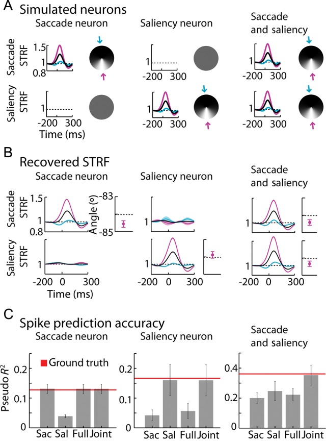
Simulations. (A) Simulated spatial and temporal filters for the 3 different kinds of neurons: purely saccade, purely saliency, and both saccade and saliency encoding. We used a fixed temporal filter (triggered on saccade onset for saccade responses and on fixation onset for saliency responses) and a fixed preferred direction (represented by the circles with shades of gray—preferred direction corresponds to the lighter shades). Blue and purple curves correspond to the temporal gains in the directions of lower (blue arrow) and higher (purple arrow) modulation of the spatio-temporal receptive fields (STRFs). We simulated spikes using behavioral data corresponding to 1 neuron of our dataset. (B) Recovered temporal filters (shaded area interval corresponds to ±2 SEM) and preferred directions (±2 SEM, 10-fold cross-validation. Black dashed line in error bar plot corresponds to the simulated/true preferred direction: direction of lighter shades of gray signaled by the purple arrow in Panel A) for saccade and for saliency using the joint model for each of the simulated neurons of Panel A. (C) Cross-validated (±2 SEM, 10-fold) pseudo R2 for each of the 4 models (saccade only, saliency only, full-saccade and joint model) for each of the 3 simulated neurons (saccade only, saliency only, and both saccade and saliency).
For the next set of simulations (as presented in Results, Fig. 8) we used data from a particular neuron (neuron 4) and we fitted the receptive fields using the saccade only model. We then used baseline and the STRF terms to simulate spike data for a new set of simulated neurons. We tested how adding Gaussian white noise to the IK-saliency affected how well we could recover saliency encoding (as measured by relative pseudo R2 between the joint model and the saccade only model). We matched the variance of the noise to the variance of the IK-saliency image. Finally, we simulated neurons that lie in the range between only saccade encoding neurons and neurons that encode equal amounts of saccade and saliency, and again tested how well we could recover saliency encoding.
Figure 8.

Statistical power analysis. (A) Relative pseudo R2 between the joint model and the movement model, (±2 SEM) as a function of the signal-to-noise ratio of the saliency definition, for a saccade only neuron and for a neuron that encodes saccade and saliency. (B) Relative pseudo R2 between the joint model and the movement model (±2 SEM), as a function of the amount of saliency that the neuron encodes relative to movement.
Results
We recorded from single neurons in the FEF of behaving monkeys while they searched for a small inconspicuous target embedded in a natural image stimulus (Fig. 1, target not shown, see Materials and Methods section). Eye movements where monitored and the monkey was rewarded with water for successfully finding the target. In the following analysis, we examine the activity of 52 FEF neurons recorded from 2 rhesus monkeys (MAS14, n = 30; MAS15, n = 22) categorized, using visual and memory-guided saccade tasks, as visual (n = 37) or visuomovement (n = 15) neurons; visual neurons have strong responses after target onset in the receptive field and visuomovement neurons are visual neurons that also have strong activity during the presaccade epoch (see Materials and Methods section—FEF cell characterization). A previous study examined saccade tuning in these data, ignoring visual information (Phillips and Segraves 2010). Here, we analyze how the activity of the neurons relates to aspects of both saccades and features of the natural scene stimuli, more specifically to a bottom-up definition of saliency.
Figure 1.
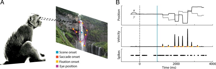
Behavioral task and data from a typical trial. (A) Monkeys were rewarded for finding the picture of a fly (not shown) embedded in natural scenes. (B) Eye position and spike trains were recorded for each trial, allowing us to model dependencies between image features, eye movement, and neural responses. Vertical dashed line marks beginning of fixation of a dot appearing at the center of the tangent screen. Blue vertical line marks the appearance of the image with embedded target. Red and yellow dots mark the beginning and end of saccades. Saccade endpoints correspond to the beginning of a new period of fixation between saccades.
We use the definition of saliency (IK-saliency) developed by Itti and Koch (2000). The IK-saliency is a traditional, bottom-up saliency map algorithm that converts images into saliency maps based upon color, intensity, and orientation on multiple spatial scales (see (Itti and Koch 2000) Materials and Methods section and Supplementary Material for details). For each of the maps, the algorithm computes how different each location or pixel is from its surround, and the map is then normalized. This leads to conspicuity maps which are then added together to define the overall saliency map. Points that are similar to the rest of the image will have low saliency while, potentially interesting points that are different from the rest of the image have high saliency (Fig. 2A,B). The resulting saliency map tends to be highly sparse with most regions of the image being unsurprising (Fig. 2A). There is a non-negligible center bias where the center of the image is more salient than the borders (Fig. 2B), an effect that is due to human photographers having a bias in their choice of pointing direction (Tseng et al. 2009). Saliency maps summarize the high dimensional properties of an image with a single dimension; the saliency or interestingness of the image as a function of space.
We first wanted to check if, as predicted by previous publications (Einhäuser et al. 2006; Berg et al. 2009), monkeys look more often at regions of the image that have high saliency. We thus plotted the standard ROC curve which quantifies how well the saccade targets can be predicted from the saliency map (Fig. 2C). We found the area under the ROC curve to be 0.587 (0.584, 0.590) (median and 95% confidence interval, bootstrap, see Materials and Methods section for details)—somewhat lower than in previous monkey free-viewing saccade experiments but above the chance level of 0.50 (Einhäuser et al. 2006). However, in our experiment, the monkey was not free-viewing the images but had a specific task: it was searching for an embedded target. This top-down goal likely makes the saccades less predictable compared with the case when only bottom-up saliency information is considered. To test if the predictive values of saliency were only due to the center bias, we compared the saliency of image locations where fixations occurred with the average saliency for that location for the remainder of the image set. We found that saliency at the fixated locations tends to be higher than at the same location in the other images (P < 10−10, Mann–Whitney test), demonstrating that the predictive value of saliency for fixation choice is due to more than just center-bias. Algorithms that calculate bottom-up saliency predict some aspects of fixation behavior but tend to be somewhat imprecise. When the task is not a free-viewing task but involves target search the predictions of bottom-up saliency maps become even more imprecise. Regarding attempts to understand how saliency relates to the activities of FEF neurons, many methods such as post/peristimulus time histograms (PSTH) rely on a well-controlled stimulus or trigger. For those methods, it would be advantageous if saliency did not predict eye movements. Here, we use a model-based, multivariate regression approach where saliency and eye movements are not required to be independent.
Saccade Representation
One of the well-established characteristics of many FEF neurons is that they are tuned to the direction of upcoming movements. To quantify this dependence on saccade direction, and test if it may be affected by search in natural images, we estimated each neuron's spatiotemporal tuning to direction of movement. The saccade-triggered PSTH for eye-movements to various octants shows that indeed, some neurons do have substantial tuning to the direction of saccade (Fig. 3A).
Figure 3.
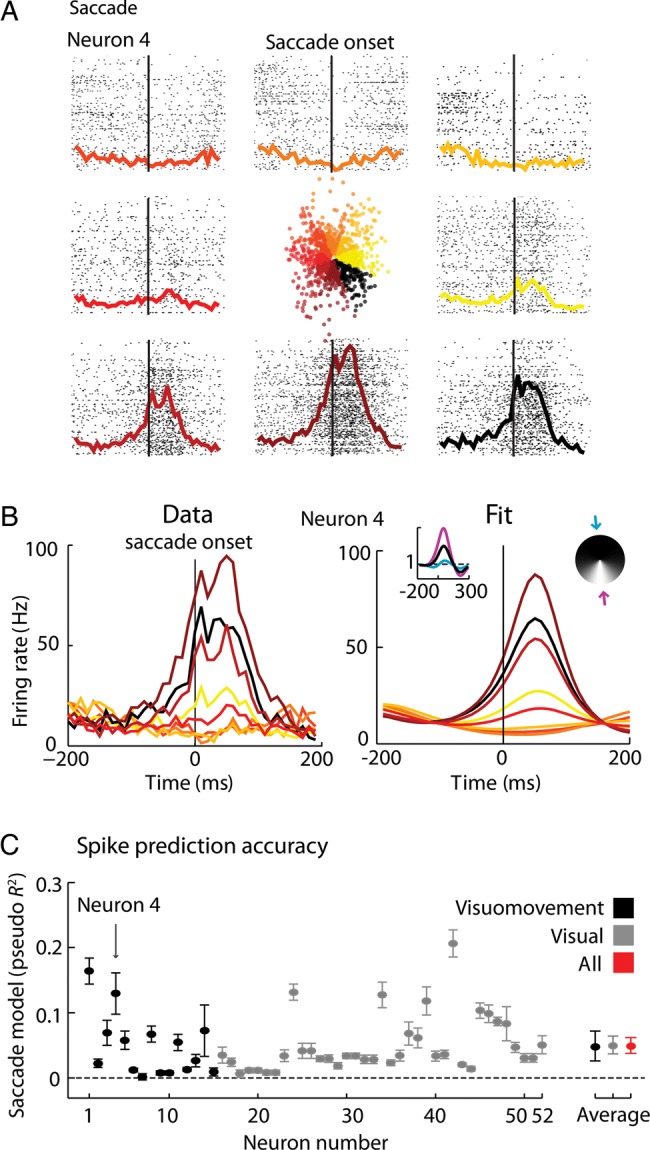
Saccade encoding. (A) Rasters sorted by direction of saccade, centered on saccade onset and the correspondent peristimulus time histograms (PSTHs) for a particular neuron (neuron 4). (B) Overlapping colored PSTHs (left), the fitted spatial and temporal receptive fields (right, insets) and correspondent reproduced PSTHs (right). Actual PSTHs were constructed using all the trials. Parameters were fitted to randomly chosen 90% of the trials and fitted PSTHs were constructed using those 90% of the trials. Blue and purple curves (right, inset) correspond to the temporal gains in the directions of lower (blue arrow) and higher (purple arrow) modulation of the spatio-temporal receptive fields (STRFs). (C) Spike prediction quality for each neuron: Pseudo R2 (±2 SEM, 10-fold cross-validation for each individual neuron; 95% bootstrap confidence intervals for the averages across the recorded population and subpopulations) of the saccade encoding model. Neurons previously classified as visuomovement and visual and respective averages (95% CI, bootstrap across neurons) are shown in black and grey, respectively (see Materials and Methods section). Global average (95% CI, bootstrap across neurons) is represented in red. Arrow signals neuron number 4, the example neuron in panels A and B. The order of the neurons is the order in which they were recorded across time but grouped by classification.
We then used a generalized linear model (GLM, see Supplementary Fig. S1B and Materials and Methods section) to explicitly model the spatiotemporal tuning to saccade direction of the neurons. The model used here (space-time separable STRF with cosine direction dependence) accurately captures the properties of the example neuron (Fig. 3B), and allows us to quantify how well-tuned each neuron is to saccades in each direction (Fig. 3C). Most of the neurons we recorded from appear to have strong saccade-related modulation, similar to previous descriptions of neurons in the FEF during simple visual tasks (e.g., Bruce and Goldberg 1985).
Vision/Saliency Representation
We next wanted to see if the same neurons might also be tuned for visual saliency. Using fixation-triggered PSTHs divided by the direction with the highest IK-saliency, we found that, indeed, some neurons seem to have substantial tuning to directions in which there are salient stimuli (Fig. 4A, but see below). Similar to the saccade direction dependence shown above, we found that a GLM based on tuning to IK-saliency accurately captured the properties of this neuron (Fig. 4B) and allowed us to quantify how well each neuron was tuned to the saliency of the stimuli (Fig. 4C). Using this saliency model, it appears that some of the neurons we recorded from do have significant tuning for salient stimuli in a particular direction.
Figure 4.
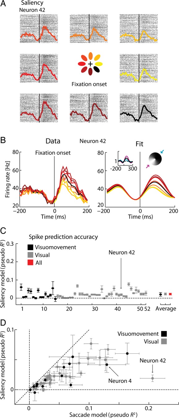
Saliency encoding. (A) Rasters and post-stimulus time histograms (PSTHs) for a particular neuron (neuron 42). Data are aligned on fixation onset, and assigned to a raster/PSTH based upon the directions where IK-saliency was elevated during the fixation interval (see Materials and Methods section for additional detail and Supplementary Fig. 3 for the analogous saccade-onset PSTHs for this neuron). (B) Overlapping colored PSTHs (left), the fitted spatial and temporal receptive fields (right, insets) and correspondent reproduced PSTHs (right). Actual PSTHs were constructed using all the trials. Parameters were fitted to randomly chosen 90% of the trials and fitted PSTHs were constructed using those 90% of the trials. Blue and purple curves (right, inset) correspond to the temporal gains in the directions of lower (blue arrow) and higher (purple arrow) modulation of the STRFs. (C) Spike prediction quality for each neuron: Pseudo R2 (±2 SEM, 10-fold cross-validation for each individual neuron; 95% bootstrap confidence intervals for the averages across the recorded population and subpopulations) for the vision/saliency encoding model. Neurons previously classified as visuomovement and visual and respective averages (±2 SEM) are shown in black and grey, respectively (see Materials and Methods section). Global average (±2 SEM) is represented in red. Arrow signals neuron 42, the example neuron in panels A and B. The order of the neurons is the order in which they were recorded across time but grouped by classification. (D) Scatter plot for spike prediction quality (±2 SEM, 10-fold cross-validation) of saccade model (same data as Fig. 3C) and saliency (same data as Fig. 4C) for each neuron.
Explaining Away Saliency Representation
So far, we have found that some neurons do appear to have tuning to saccade and also tuning to the direction in which there are salient stimuli. For most neurons, saccade direction alone provides a better model of spiking than saliency alone (Fig. 4D); however, since these 2 variables are correlated, the independent analyses above may be confounded. We have shown that monkeys tend to make saccades toward more salient targets, even during natural scene search. This means that if FEF neurons encode only saccade movement, their activity might still be correlated with saliency. Furthermore, fixation onset times and saccade onset times are also highly correlated, which may make it difficult to disambiguate the effects of saccades and saliency on spiking activity.
We thus implemented a GLM that predicts spikes based on saccade and saliency at the same time. This approach allows us to take advantage of a statistical effect called explaining away. If the spikes could be fully described by saliency then the system would put no weight on saccade and vice versa. As the saccades and saliency are not perfectly correlated, such a joint model will determine which of the 2 factors is, statistically, a more direct explanation of a neuron's firing.
For essentially all of the recorded neurons, we find that adding a spatiotemporal saliency receptive field to the saccade model does not improve the spike prediction accuracy (Fig. 5). A model that uses only saccade and a model that uses both saccade and saliency perform almost equally well (Fig. 5A,B, center panels)—in contrast, considering both saccade and saliency improves the performance relative to considering only saliency (Fig. 5A,B, left panels). In fact, the apparent saliency related modulation (Figs 4A,B and 5C, first and second columns) can be reproduced using motor information only (Fig. 5C, fourth column). Saccade covariates of the joint model can capture the trial-by-trial variability better than the saliency only model which just smears the spiking activity (Fig. 5C, fourth and third columns, respectively). As saccade duration has some variability (see Supplementary Fig. S2B), we tested a GLM that adds a purely temporal response centered at the end of the saccade to the saccade-only model: the full-saccade model. We find that it completely explains the saliency modulation for all neurons (Fig. 5A,B, right panels)—the saliency-related covariates do not add any predictive power to the full-saccade model. In other words, when modeling activities carefully, there is absolutely no sign of bottom-up saliency (Itti and Koch 2000) encoding.
Figure 5.

Explaining away. (A) Scatter plots of the spike prediction accuracy (±2 SEM, 10-fold cross-validation, see Materials and Methods section) under the saliency-only (left)/saccade-only (center)/full-saccade (right) and joint models. The saccade-only, saliency-only and full-saccade models are represented on the x-axis and the joint saccade in the y-axis. “n4” and “n42” denote neurons 4 and 42, the example neurons of Figures 3 and 4, respectively. (B) Relative pseudo R2 between the joint model and the saliency model (left)/saccade model (center)/full saccade model (right) (±2 SEM, 10-fold cross-validation for each individual neuron; 95% bootstrap confidence intervals for the averages across the recorded population and subpopulations). Arrows signal neurons 4 and 42, the example neurons of Figures 3 and 4 respectively. Note different y-axis scales for left versus center and right panels. The order of the neurons is the order in which they were recorded across time but grouped by classification. (C) Actual spikes and PSTHs (1st column) and predicted firing rates and PSTHs for saliency only model (2nd column), joint model using saliency covariates only (3rd column) and joint model using saccade covariates only (4th column) for the example neuron of Figure 4 (neuron 42). Parameters were fitted to 50% of the trials and the data shown (both actual spikes and predicted firing rates) correspond to spikes and covariates of the remaining 50% of data (testing set). Upper panels show raw data and predicted firing rates from 340 fixations of the test set where the IK-saliency in the lower-left octant area of the image relative to the point of fixation was positive (see Materials and Methods section). Lower panels show PSTHs for all directions.
The absence of improvement in spike prediction accuracy was not caused by the higher number of parameters in the joint model, since there is minimal overfitting (Fig. 6A,B). Even though the full-saccade model explains away the saliency tuning modulation at fixation onset, it does not completely explain away saccade direction modulation at the end of the saccade (also see Supplementary Material and Supplementary Fig. S4). Furthermore, we checked that explaining away is robust within a considerable range of parameterizations of the TRFs (Supplementary Fig. S5). Thus, our finding that saliency is not represented in the FEF is not due to overfitting.
Figure 6.
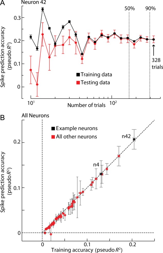
Model sensitivity and overfitting analysis. (A) Average of spike prediction accuracy (±SEM, 10-fold cross-validation) for the joint model on test data and on training data, as a function of the amount of data used. Total number of trials for this specific neuron is 328. Dashed vertical lines indicate thresholds for 50% and 90% for the trials. (B) Over-fitting analysis for the whole population. Error bars in both dimensions are ±2 SEM.
We observed that, for most of the neurons, saliency information alone allows some prediction of neural activity (Fig. 4C). In fact, the spatiotemporal terms of the saliency model add predictive power (as measured by the pseudo R2, P < 0.05, bootstrap), to a model that considers only the purely temporal terms centered at fixation onset. However, the modulation related to saliency was explained away by including saccade information (Fig. 5A,B). The fact that saliency related tuning is explained away seems surprising, since the relationship between saccades and saliency, although present, is fairly weak in our natural scene search task (Fig. 2C). Even the apparently large effects in the saliency PSTHs (Fig. 4A,B) and spike prediction (Figs 4C and 5A) seem to be well explained based on these correlations (Fig. 5A–C). Part of the directional tuning may be explained by the fact that the center of images tends to be more salient than the periphery (Fig. 2B), and when fixation is at the edge of the image saccades toward the center become more likely. Furthermore, saccade onset and fixation onset happen close in time and saccade durations have some variability (Supplementary Fig. S2B). Neural responses are driven by a range of different factors. Ignoring some factors may lead us to draw wrong conclusions, but by modeling these factors together we can disambiguate which factors truly relate to the responses.
Simulations
It could be that we failed to find true saliency responses in FEF because our data analysis routines did not correctly handle the correlations between the variables. We thus simulated equivalent amounts of data using a range of models: a purely saccade neuron, a purely saliency neuron and a neuron that encodes saccade and saliency simultaneously (Fig. 7A, see Materials and Methods section for details). We then asked if our methods would be able to recover the spatiotemporal tuning of these simulated neurons. Using the same GLM approach as above, we find that we can readily detect tuning to preferred saccade direction or saliency direction (Fig. 7B,C) and the spatially and non-spatially dependent temporal responses. If the neurons in the actual FEF sample were truly tuned to the definition of saliency we are using, then these simulations demonstrate that we should have been able to reconstruct this dependence.
Lastly, it might simply be that our analysis was underpowered and more data would have been necessary to observe modulations in firing rate due to saliency. To test for this possibility, we simulated neurons using the STRF component of the fitted receptive field to data of a particular neuron (neuron 4, Fig. 4B; see Materials and Methods section for details). We degraded the signal quality in our simulated neurons in 2 ways: 1) We made the definition of saliency used in the models worse by adding noise to the IK-saliency definition and 2) We simulated neurons that were mostly tuned to saccade movement with progressively weaker modulation due to saliency. We found that even if saliency signals were highly corrupted (SNR ∼ 0.1) the amount of data available here should have been sufficient to resolve saliency related tuning (Fig. 8A). We also found that even if the saliency tuning is substantially smaller than saccade tuning (by a factor of ∼3) these effects should have been picked up (Fig. 8B). Concretely, we can say that if IK-saliency had at least 25% influence on the neural activity of this neuron then we should have had more than 95% probability of finding it.
Discussion
In this study, we examined the activity of FEF neurons to determine whether or not they represent bottom-up saliency while a monkey searches for small targets embedded in natural scenes. We found that saliency is mildly predictive of eye-movement direction during natural scene search but it appears not to be a determinant of FEF activity when other correlated, saccade-related covariates are properly taken into account. Our finding that FEF does not appear to represent bottom-up saliency suggests that the activity of the FEF may be dominated by top-down target-selection and saccade planning.
Our study has used eye movements during natural scene viewing to ask if neurons in the FEF represent bottom-up saliency. There are, of course, factors that limit the interpretation of our results.
Caveat 1: Our definition of saliency may differ from the actual representation of bottom-up saliency used by the FEF. We have employed a commonly used definition of bottom-up saliency (Itti and Koch 2000). Past research has shown that most definitions of bottom-up saliency lead to saliency maps that are highly correlated with one another and are often difficult to disambiguate behaviorally (Borji et al. 2012). This is because most computational definitions of bottom-up saliency effectively ask how dissimilar image patches are from the rest of the image and the specific metric of similarity often has little influence in such cases (Schölkopf and Smola 2002). Therefore, it seems unlikely that other definitions of bottom-up saliency would have improved our ability to observe saliency tuning in FEF neurons.
Caveat 2: Our results show that if bottom-up saliency is represented in the FEF during natural scene search it is only explaining a tiny proportion of the overall activity. This does not imply that there is no representation of bottom-up saliency, nor does it imply that this proportion would be as small if it was a free-viewing task; just that our results support a weak representation. However, given that activity in the FEF is sufficiently strongly dominated by planning, it appears that bottom-up saliency representation is not a central function of FEF.
Previous research using artificial stimuli has suggested that significant activity in the FEF is devoted to the representation of visual saliency, noting that salient objects within the receptive field of an FEF cell may elicit high activity even without a saccade that actually ends in the receptive field (Thompson et al. 1996, 1997; Bichot and Schall 1999; Murthy et al. 2001). However, our results suggest that bottom-up saliency is not represented in the FEF. Furthermore, other studies using natural scenes suggest that visual cells do not respond to stimuli unless their receptive field contains the target of a future saccade (Burman and Segraves 1994; Phillips and Segraves 2010). How can this difference be explained? We suggest a couple of possible explanations for this apparent contradiction.
First, the eye-movement field has had some difficulty to adhere to a uniform definition of saliency, and generally includes a combination of bottom-up and top-down—including target relevance and the probability of a saccade—factors within the realm of saliency (but see Melloni et al. 2012). This ambiguity makes it difficult to directly relate bottom-up saliency to activity in the FEF.
Second, we expect activity to be much higher for non-targets in a search task where the number of distractors is small (see McPeek and Keller 2002). Given the small number of targets and the exceptionally high levels of saliency used in typical experiments, results may not generalize to search in natural scenes. Furthermore, it may be that highly salient stimuli trigger implicit planning of saccades that is later aborted, and hence, that the activity of a visual cell represents the amount of covert attention allocated to that location. Future work should directly compare the responses of FEF neurons to the traditional artificial salient stimuli and to more natural stimuli.
There are many computational definitions of the top-down factors that are likely to be represented in the FEF. The oculomotor system takes into account what the task-relevant target looks like (the relevance) (Serre et al. 2007) and the likely locations of the target given the scene context (the gist) (Torralba et al. 2006; Vogel and Schiele 2007). Several studies have shown that most of search is driven by task-demands (Yarbus 1967) and that it can override sensory-driven (bottom-up) saliency almost entirely (Einhäuser et al. 2008). In our task the monkey was not free-viewing but searching for an embedded target. Looking for representations of these top-down influences is possible with the methods presented here and would be an exciting topic for future research.
If bottom-up saliency is not represented in the FEF but it is important for the selection of saccades, it should be represented somewhere else. A model of a processing stream for visual saliency suggests a succession of stages in the visual-motor pathway from V1 to extrastriate visual cortex and on to areas LIP and FEF (Soltani and Koch 2010). A recent imaging study has suggested that V1 represents bottom-up saliency while FEF is involved with target enhancement (Melloni et al. 2012). There have been reports supporting the existence of visual saliency maps in V4 (Mazer and Gallant 2003; Burrows and Moore 2009; Zhou and Desimone 2011), LIP (Gottlieb et al. 1998; Constantinidis and Steinmetz 2005; Arcizet et al. 2011), and FEF (Schall and Thompson 1999; Thompson and Bichot 2005; Wardak et al. 2010). A true bottom-up saliency map must represent the conspicuity of stimuli in the visual field, independent of the individual stimulus features themselves. However, given our results about the subtle ways by which apparent saliency tuning may arise, it seems fair to state that the question of if and where the brain represents saliency has not yet received a sufficient answer. It is not clear where in the visuomotor system relevance/target-matching is computed, but this study provides a counter-point to the hyper-salient tasks used in artificial experiments.
The approach taken here provides a template for how multiple factors that simultaneously might affect neural responses can be analyzed. Specifically, our analysis attempts to define what it means to say that the FEF encodes saliency when other correlated variables, such as saccade planning, may also be encoded by the same neurons. Here we used a precise definition of bottom-up saliency from the computational literature to quantify the extent to which FEF neurons represent bottom-up visual saliency during natural scene search. We found that it is not strongly represented. Instead, saccade planning and execution dominate the neural responses. This emphasizes the role of the FEF as a premotor structure, where neural activity encodes information about the importance of various spatial locations as potential saccade targets, independent of the visual properties of those locations.
Supplementary Material
Supplementary material can be found at: http://www.cercor.oxfordjournals.org/.
Funding
This work was supported by the Fundação para a Ciência e Tecnologia (SFRH/BD/33525/2008 to H.L.F.), the National Institutes of Health (1R01NS063399, 2P01NS044393, 5R01EY008212 and 5T32EY007128, 1R01EY021579) and by the National Science Foundation (CRCNS program).
Supplementary Material
Notes
Conflict of Interest: None declared.
References
- Ahrens MB, Paninski L, Sahani M. Inferring input nonlinearities in neural encoding models. Network. 2008;19:35–67. doi: 10.1080/09548980701813936. [DOI] [PubMed] [Google Scholar]
- Arcizet F, Mirpour K, Bisley JW. A pure salience response in posterior parietal cortex. Cereb Cortex. 2011;21:2498–2506. doi: 10.1093/cercor/bhr035. [DOI] [PMC free article] [PubMed] [Google Scholar]
- Bell AJ, Sejnowski TJ. The “independent components” of natural scenes are edge filters. Vision Res. 1997;37:3327–3338. doi: 10.1016/S0042-6989(97)00121-1. [DOI] [PMC free article] [PubMed] [Google Scholar]
- Bengio Y, Grandvalet Y. No unbiased estimator of the variance of k-fold cross-validation. J Mach Learn Res. 2004;5:1089–1105. [Google Scholar]
- Berg DJ, Boehnke SE, Marino RA, Munoz DP, Itti L. Free viewing of dynamic stimuli by humans and monkeys. J Vis. 2009;9:1–15. doi: 10.1167/9.5.19. [DOI] [PubMed] [Google Scholar]
- Betsch BY, Einhäuser W, Körding KP, König P. The world from a cat's perspective–statistics of natural videos. Biological cybernetics. 2004;90:41–50. doi: 10.1007/s00422-003-0434-6. [DOI] [PubMed] [Google Scholar]
- Bichot NP, Schall JD, Thompson KG. Visual feature selectivity in frontal eye fields induced by experience in mature macaques. Nature. 1996;381:697–699. doi: 10.1038/381697a0. [DOI] [PubMed] [Google Scholar]
- Bichot NP, Schall JD. Effects of similarity and history on neural mechanisms of visual selection. Nature Neurosci. 1999;2:549–554. doi: 10.1038/9205. [DOI] [PubMed] [Google Scholar]
- Bizzi E. Discharge of frontal eye field neurons during saccadic and following eye movements in unanesthetized monkeys. Exp Brain Res. 1968;6:69–80. doi: 10.1007/BF00235447. [DOI] [PubMed] [Google Scholar]
- Bizzi E, Schiller PH. Single unit activity in the frontal eye fields of unanesthetized monkeys during head and eye movement. Exp Brain Res. 1970;10:151–158. doi: 10.1007/BF00234728. [DOI] [PubMed] [Google Scholar]
- Borji A, Sihite D, Itti L. Quantitative analysis of human-model agreement in visual saliency modeling: a comparative study. IEEE Trans Image Processing. 2012;22:55–69. doi: 10.1109/TIP.2012.2210727. [DOI] [PubMed] [Google Scholar]
- Bruce CJ, Goldberg ME. Primate frontal eye fields. I. Single neurons discharging before saccades. J Neurophysiol. 1985;53:603. doi: 10.1152/jn.1985.53.3.603. [DOI] [PubMed] [Google Scholar]
- Burman DD, Segraves MA. Primate frontal eye field activity during natural scanning eye movements. J Neurophysiol. 1994;71:1266–1271. doi: 10.1152/jn.1994.71.3.1266. [DOI] [PubMed] [Google Scholar]
- Burrows BE, Moore T. Influence and limitations of popout in the selection of salient visual stimuli by area V4 neurons. J Neurosci. 2009;29:15169–15177. doi: 10.1523/JNEUROSCI.3710-09.2009. [DOI] [PMC free article] [PubMed] [Google Scholar]
- Cave KR, Wolfe JM. Modeling the role of parallel processing in visual search. Cognit Psychol. 1990;22:225–271. doi: 10.1016/0010-0285(90)90017-X. [DOI] [PubMed] [Google Scholar]
- Constantinidis C, Steinmetz MA. Posterior parietal cortex automatically encodes the location of salient stimuli. J Neurosci. 2005;25:233–238. doi: 10.1523/JNEUROSCI.3379-04.2005. [DOI] [PMC free article] [PubMed] [Google Scholar]
- Crist CF, Yamasaki DSG, Komatsu H, Wurtz RH. A grid system and a microsyringe for single cell recording. J Neurosci Methods. 1988;26:117–122. doi: 10.1016/0165-0270(88)90160-4. [DOI] [PubMed] [Google Scholar]
- Dias EC, Kiesau M, Segraves MA. Acute activation and inactivation of macaque frontal eye field with GABA-related drugs. J Neurophysiol. 1995;74:2744–2748. doi: 10.1152/jn.1995.74.6.2744. [DOI] [PubMed] [Google Scholar]
- Dias EC, Segraves MA. Muscimol-induced inactivation of monkey frontal eye field: effects on visually and memory-guided saccades. J Neurophysiol. 1999;81:2191–2214. doi: 10.1152/jn.1999.81.5.2191. [DOI] [PubMed] [Google Scholar]
- Ehinger KA, Hidalgo-Sotelo B, Torralba A, Oliva A. Modelling search for people in 900 scenes: a combined source model of eye guidance. Vis Cogn. 2009;17:945–978. doi: 10.1080/13506280902834720. [DOI] [PMC free article] [PubMed] [Google Scholar]
- Einhäuser W, Kruse W, Hoffmann KP, König P. Differences of monkey and human overt attention under natural conditions. Vision Res. 2006;46:1194–1209. doi: 10.1016/j.visres.2005.08.032. [DOI] [PubMed] [Google Scholar]
- Einhäuser W, Rutishauser U, Koch C. Task-demands can immediately reverse the effects of sensory-driven saliency in complex visual stimuli. J Vis. 2008;8:1–19. doi: 10.1167/8.2.2. [DOI] [PubMed] [Google Scholar]
- Elazary L, Itti L. Interesting objects are visually salient. J Vis. 2008;8:1–15. doi: 10.1167/8.3.3. [DOI] [PubMed] [Google Scholar]
- Everling S, Munoz DP. Neuronal correlates for preparatory set associated with pro-saccades and anti-saccades in the primate frontal eye field. J Neurosci. 2000;20:387–400. doi: 10.1523/JNEUROSCI.20-01-00387.2000. [DOI] [PMC free article] [PubMed] [Google Scholar]
- Fecteau JH, Munoz DP. Salience, relevance, and firing: a priority map for target selection. Trends Cogn Sci. 2006;10:382–390. doi: 10.1016/j.tics.2006.06.011. [DOI] [PubMed] [Google Scholar]
- Ferrier D. Experiments on the brains of monkeys. Phil Trans London (Croonian Lecture) 1875;165:433–488. doi: 10.1098/rstl.1875.0016. [DOI] [Google Scholar]
- Foulsham T, Barton JJS, Kingstone A, Dewhurst R, Underwood G. Modeling eye movements in visual agnosia with a saliency map approach: bottom-up guidance or top-down strategy? Neural Netw. 2011;24:665–677. doi: 10.1016/j.neunet.2011.01.004. [DOI] [PubMed] [Google Scholar]
- Georgopoulos AP, Kalaska JF, Caminiti R, Massey JT. On the relations between the direction of two-dimensional arm movements and cell discharge in primate motor cortex. J Neurosci. 1982;2:1527. doi: 10.1523/JNEUROSCI.02-11-01527.1982. [DOI] [PMC free article] [PubMed] [Google Scholar]
- Gottlieb JP, Kusunoki M, Goldberg ME. The representation of visual salience in monkey parietal cortex. Nature. 1998;391:481–484. doi: 10.1038/35135. [DOI] [PubMed] [Google Scholar]
- Harris KD, Csicsvari J, Hirase H, Dragoi G, Buzsáki G. Organization of cell assemblies in the hippocampus. Nature. 2003;424:552–556. doi: 10.1038/nature01834. [DOI] [PubMed] [Google Scholar]
- Haslinger R, Pipa G, Lima B, Singer W, Brown EN, Neuenschwander S. Context matters: the illusive simplicity of Macaque V1 receptive fields. PLOS One. 2012;7:e39699. doi: 10.1371/journal.pone.0039699. [DOI] [PMC free article] [PubMed] [Google Scholar]
- Hatsopoulos NG, Xu Q, Amit Y. Encoding of movement fragments in the motor cortex. J Neurosci. 2007;27:5105. doi: 10.1523/JNEUROSCI.3570-06.2007. [DOI] [PMC free article] [PubMed] [Google Scholar]
- Hays AV, Richmond BJ, Optican LM. Unix-based multiple-process system, for real-time data acquisition and control. WESCON Conf Proc. 1982;2:1–10. [Google Scholar]
- Heinzl H, Mittlböck M. Pseudo R-squared measures for Poisson regression models with over-or underdispersion. Comput Stat Data Anal. 2003;44:253–271. doi: 10.1016/S0167-9473(03)00062-8. [DOI] [Google Scholar]
- Howard IS, Ingram JN, Kording KP, Wolpert DM. Statistics of natural movements are reflected in motor errors. J Neurophysiol. 2009;102:1902–1910. doi: 10.1152/jn.00013.2009. [DOI] [PMC free article] [PubMed] [Google Scholar]
- Hyvarinen A, Hurri J, Vayrynen J. Bubbles: a unifying framework for low-level statistical properties of natural image sequences. J Opt Soc Am A Opt Image Sci Vis. 2003;20:1237–1252. doi: 10.1364/JOSAA.20.001237. [DOI] [PubMed] [Google Scholar]
- Ingram JN, Körding KP, Howard IS, Wolpert DM. The statistics of natural hand movements. Exp Brain Res. 2008;188:223–236. doi: 10.1007/s00221-008-1355-3. [DOI] [PMC free article] [PubMed] [Google Scholar]
- Itti L, Baldi P. Bayesian surprise attracts human attention. Adv Neural Inform Process Syst. 2006;18:547. doi: 10.1016/j.visres.2008.09.007. [DOI] [PMC free article] [PubMed] [Google Scholar]
- Itti L, Koch C. Computational modelling of visual attention. Nat Rev Neurosci. 2001;2:194–203. doi: 10.1038/35058500. [DOI] [PubMed] [Google Scholar]
- Itti L, Koch C. A saliency-based search mechanism for overt and covert shifts of visual attention. Vision Res. 2000;40:1489–1506. doi: 10.1016/S0042-6989(99)00163-7. [DOI] [PubMed] [Google Scholar]
- Judge SJ, Richmond BJ, Chu FC. Implantation of magnetic search coils for measurement of eye position: an improved method. Vision Res. 1980;20:535–538. doi: 10.1016/0042-6989(80)90128-5. [DOI] [PubMed] [Google Scholar]
- Kayser C, Kording KP, Konig P. Processing of complex stimuli and natural scenes in the visual cortex. Curr Opin Neurobiol. 2004;14:468–473. doi: 10.1016/j.conb.2004.06.002. [DOI] [PubMed] [Google Scholar]
- Kayser C, Nielsen KJ, Logothetis NK. Fixations in natural scenes: interaction of image structure and image content. Vision Res. 2006;46:2535–2545. doi: 10.1016/j.visres.2006.02.003. [DOI] [PubMed] [Google Scholar]
- Kayser C, Salazar R, König P. Responses to natural scenes in cat V1. J Neurophysiol. 2003;90:1910–1920. doi: 10.1152/jn.00195.2003. [DOI] [PubMed] [Google Scholar]
- Koch C, Ullman S. Shifts in selective visual attention: towards the underlying neural circuitry. Hum Neurobiol. 1985;4:219–227. [PubMed] [Google Scholar]
- Land MF, Hayhoe M. In what ways do eye movements contribute to everyday activities? Vision Res. 2001;41:3559–3565. doi: 10.1016/S0042-6989(01)00102-X. [DOI] [PubMed] [Google Scholar]
- Lewicki MS. Efficient coding of natural sounds. Nat Neurosci. 2002;5:356–363. doi: 10.1038/nn831. [DOI] [PubMed] [Google Scholar]
- MacEvoy SP, Hanks TD, Paradiso MA. Macaque V1 activity during natural vision: effects of natural scenes and saccades. J Neurophysiol. 2008;99:460–472. doi: 10.1152/jn.00612.2007. [DOI] [PMC free article] [PubMed] [Google Scholar]
- Mazer JA, Gallant JL. Goal-related activity in V4 during free viewing visual search. Evidence for a ventral stream visual salience map. Neuron. 2003;40:1241–1250. doi: 10.1016/S0896-6273(03)00764-5. [DOI] [PubMed] [Google Scholar]
- McPeek RM, Keller EL. Saccade target selection in the superior colliculus during a visual search task. J Neurophysiol. 2002;88:2019–2034. doi: 10.1152/jn.2002.88.4.2019. [DOI] [PubMed] [Google Scholar]
- Melloni L, van Leeuwen S, Alink A, Müller NG. Interaction between bottom-up saliency and top-down control: how saliency maps are created in the human brain. Cerebr Cortex. 2012;22:2943–2952. doi: 10.1093/cercor/bhr384. [DOI] [PubMed] [Google Scholar]
- Mohler CW, Goldberg ME, Wurtz RH. Visual receptive fields of frontal eye field neurons. Brain Res. 1973;61:385–389. doi: 10.1016/0006-8993(73)90543-X. [DOI] [PubMed] [Google Scholar]
- Murthy A, Thompson KG, Schall JD. Dynamic dissociation of visual selection from saccade programming in frontal eye field. J Neurophysiol. 2001;86:2634–2637. doi: 10.1152/jn.2001.86.5.2634. [DOI] [PubMed] [Google Scholar]
- Oliva A, Torralba A, Castelhano MS, Henderson JM. Top-down control of visual attention in object detection. Proceedings of the 2003 International Conference on Image Processing; 2003. pp. 253–256. [Google Scholar]
- Olshausen B, Field D. Emergence of simple-cell receptive field properties by learning a sparse code for natural images. Nature. 1996;381:607–609. doi: 10.1038/381607a0. [DOI] [PubMed] [Google Scholar]
- O'Shea J, Muggleton NG, Cowey A, Walsh V. Timing of target discrimination in human frontal eye fields. J Cogn Neurosci. 2004;16:1060–1067. doi: 10.1162/0898929041502634. [DOI] [PubMed] [Google Scholar]
- Pearl J. Probabilistic reasoning in intelligent systems: networks of plausible inference. San Francisco: Morgan Kaufmann; 1988. [Google Scholar]
- Peng X, Sereno ME, Silva AK, Lehky SR, Sereno AB. Shape selectivity in primate frontal eye field. J Neurophysiol. 2008;100:796–814. doi: 10.1152/jn.01188.2007. [DOI] [PMC free article] [PubMed] [Google Scholar]
- Phillips A, Segraves M. Predictive activity in Macaque frontal eye field neurons during natural scene searching. J Neurophysiol. 2010;103:1238. doi: 10.1152/jn.00776.2009. [DOI] [PMC free article] [PubMed] [Google Scholar]
- Pillow JW, Shlens J, Paninski L, Sher A, Litke AM, Chichilnisky E, Simoncelli EP. Spatio-temporal correlations and visual signalling in a complete neuronal population. Nature. 2008;454:995–999. doi: 10.1038/nature07140. [DOI] [PMC free article] [PubMed] [Google Scholar]
- Ray S, Pouget P, Schall JD. Functional distinction between visuomovement and movement neurons in macaque frontal eye field during saccade countermanding. J Neurophysiol. 2009;102:3091–3100. doi: 10.1152/jn.00270.2009. [DOI] [PMC free article] [PubMed] [Google Scholar]
- Robinson DA. A method of measuring eye movement using a scleral search coil in a magnetic field. IEEE Trans Bio-Med Electron BME. 1963;10:137–145. doi: 10.1109/TBMEL.1963.4322822. [DOI] [PubMed] [Google Scholar]
- Rolls ET, Tovee MJ. Sparseness of the neuronal representation of stimuli in the primate temporal visual cortex. J Neurophysiol. 1995;73:713–726. doi: 10.1152/jn.1995.73.2.713. [DOI] [PubMed] [Google Scholar]
- Saleh M, Takahashi K, Amit Y, Hatsopoulos NG. Encoding of coordinated grasp trajectories in primary motor cortex. J Neurosci. 2010;30:17079. doi: 10.1523/JNEUROSCI.2558-10.2010. [DOI] [PMC free article] [PubMed] [Google Scholar]
- Sato T, Murthy A, Thompson KG, Schall JD. Search efficiency but not response interference affects visual selection in frontal eye field. Neuron. 2001;30:583–591. doi: 10.1016/S0896-6273(01)00304-X. [DOI] [PubMed] [Google Scholar]
- Sato TR, Schall JD. Effects of stimulus-response compatibility on neural selection in frontal eye field. Neuron. 2003;38:637–648. doi: 10.1016/S0896-6273(03)00237-X. [DOI] [PubMed] [Google Scholar]
- Schall JD. Neuronal activity related to visually guided saccades in the frontal eye fields of rhesus monkeys: comparison with supplementary eye fields. J Neurophysiol. 1991;66:559–579. doi: 10.1152/jn.1991.66.2.559. [DOI] [PubMed] [Google Scholar]
- Schall JD, Hanes DP. Neural basis of saccade target selection in frontal eye field during visual search. Nature. 1993;366:467–469. doi: 10.1038/366467a0. [DOI] [PubMed] [Google Scholar]
- Schall JD, Hanes DP, Thompson KG, King DJ. Saccade target selection in frontal eye field of macaque. I. Visual and premovement activation. J Neurosci. 1995;15:6905–6918. doi: 10.1523/JNEUROSCI.15-10-06905.1995. [DOI] [PMC free article] [PubMed] [Google Scholar]
- Schall JD, Thompson KG. Neural selection and control of visually guided eye movements. Annu Rev Neurosci. 1999;22:241–259. doi: 10.1146/annurev.neuro.22.1.241. [DOI] [PubMed] [Google Scholar]
- Schiller PH, True SD, Conway JL. Deficits in eye movements following frontal eye field and superior colliculus ablations. J Neurophysiol. 1980;44:1175–1189. doi: 10.1152/jn.1980.44.6.1175. [DOI] [PubMed] [Google Scholar]
- Schölkopf B, Smola AJ. Learning with kernels: support vector machines, regularization, optimization, and beyond. Cambridge, MA: MIT Press; 2002. [Google Scholar]
- Schwartz O, Simoncelli EP. Natural signal statistics and sensory gain control. Nat Neurosci. 2001;4:819–825. doi: 10.1038/90526. [DOI] [PubMed] [Google Scholar]
- Segraves MA. Activity of monkey frontal eye field neurons projecting to oculomotor regions of the pons. J Neurophysiol. 1992;68:1967–1985. doi: 10.1152/jn.1992.68.6.1967. [DOI] [PubMed] [Google Scholar]
- Segraves MA, Goldberg ME. Functional properties of corticotectal neurons in the monkey's frontal eye field. J Neurophysiol. 1987;58:1387–1419. doi: 10.1152/jn.1987.58.6.1387. [DOI] [PubMed] [Google Scholar]
- Segraves MA, Park K. The relationship of monkey frontal eye field activity to saccade dynamics. J Neurophysiol. 1993;69:1880–1889. doi: 10.1152/jn.1993.69.6.1880. [DOI] [PubMed] [Google Scholar]
- Serences JT, Yantis S. Selective visual attention and perceptual coherence. Trends Cogn Sci. 2006;10:38–45. doi: 10.1016/j.tics.2005.11.008. [DOI] [PubMed] [Google Scholar]
- Serre T, Wolf L, Bileschi S, Riesenhuber M, Poggio T. Robust object recognition with cortex-like mechanisms. IEEE Trans Pattern Anal Mach Intelligence. 2007:411–426. doi: 10.1109/TPAMI.2007.56. [DOI] [PubMed] [Google Scholar]
- Sharpee T, Rust NC, Bialek W. Analyzing neural responses to natural signals: maximally informative dimensions. Neural Comput. 2004;16:223–250. doi: 10.1162/089976604322742010. [DOI] [PubMed] [Google Scholar]
- Smith EC, Lewicki MS. Efficient auditory coding. Nature. 2006;439:978–982. doi: 10.1038/nature04485. [DOI] [PubMed] [Google Scholar]
- Smyth D, Willmore B, Baker GE, Thompson ID, Tolhurst DJ. The receptive-field organization of simple cells in primary visual cortex of ferrets under natural scene stimulation. J Neurosci. 2003;23:4746–4759. doi: 10.1523/JNEUROSCI.23-11-04746.2003. [DOI] [PMC free article] [PubMed] [Google Scholar]
- Soltani A, Koch C. Visual saliency computations: mechanisms, constraints, and the effect of feedback. J Neurosci. 2010;30:12831–12843. doi: 10.1523/JNEUROSCI.1517-10.2010. [DOI] [PMC free article] [PubMed] [Google Scholar]
- Sommer MA, Tehovnik EJ. Reversible inactivation of macaque frontal eye field. Exp Brain Res. 1997;116:229–249. doi: 10.1007/PL00005752. [DOI] [PubMed] [Google Scholar]
- Sommer MA, Wurtz RH. Composition and topographic organization of signals sent from the frontal eye field to the superior colliculus. J Neurophysiol. 2000;83:1979–2001. doi: 10.1152/jn.2000.83.4.1979. [DOI] [PubMed] [Google Scholar]
- Sommer MA, Wurtz RH. Frontal eye field sends delay activity related to movement, memory, and vision to the superior colliculus. J Neurophysiol. 2001;85:1673–1685. doi: 10.1152/jn.2001.85.4.1673. [DOI] [PubMed] [Google Scholar]
- Srivastava A, Lee AB, Simoncelli EP, Zhu SC. On advances in statistical modeling of natural images. J Math Imaging Vis. 2003;18:17–33. doi: 10.1023/A:1021889010444. [DOI] [Google Scholar]
- Suzuki H, Azuma M. Prefrontal neuronal activity during gazing at a light spot in the monkey. Brain Res. 1977;126:497–508. doi: 10.1016/0006-8993(77)90600-X. [DOI] [PubMed] [Google Scholar]
- Theunissen FE, David SV, Singh NC, Hsu A, Vinje WE, Gallant JL. Estimating spatio-temporal receptive fields of auditory and visual neurons from their responses to natural stimuli. Network. 2001;12:289–316. [PubMed] [Google Scholar]
- Theunissen FE, Sen K, Doupe AJ. Spectral-temporal receptive fields of nonlinear auditory neurons obtained using natural sounds. J Neurosci. 2000;20:2315–2331. doi: 10.1523/JNEUROSCI.20-06-02315.2000. [DOI] [PMC free article] [PubMed] [Google Scholar]
- Thompson KG, Bichot NP. A visual salience map in the primate frontal eye field. Progr Brain Res. 2005;147:249–262. doi: 10.1016/S0079-6123(04)47019-8. [DOI] [PubMed] [Google Scholar]
- Thompson KG, Bichot NP, Sato TR. Frontal eye field activity before visual search errors reveals the integration of bottom-up and top-down salience. J Neurophysiol. 2005;93:337. doi: 10.1152/jn.00330.2004. [DOI] [PMC free article] [PubMed] [Google Scholar]
- Thompson KG, Bichot NP, Schall JD. Dissociation of visual discrimination from saccade programming in macaque frontal eye field. J Neurophysiol. 1997;77:1046–1050. doi: 10.1152/jn.1997.77.2.1046. [DOI] [PubMed] [Google Scholar]
- Thompson KG, Hanes DP, Bichot NP, Schall JD. Perceptual and motor processing stages identified in the activity of macaque frontal eye field neurons during visual search. J Neurophysiol. 1996;76:4040–4055. doi: 10.1152/jn.1996.76.6.4040. [DOI] [PubMed] [Google Scholar]
- Torralba A, Oliva A, Castelhano MS, Henderson JM. Contextual guidance of eye movements and attention in real-world scenes: the role of global features in object search. Psychol Rev. 2006;113:766. doi: 10.1037/0033-295X.113.4.766. [DOI] [PubMed] [Google Scholar]
- Treisman A. Features and objects: the fourteenth Bartlett memorial lecture. Q J Exp Psychol A. 1988;40:201–237. doi: 10.1080/02724988843000104. [DOI] [PubMed] [Google Scholar]
- Truccolo W, Eden UT, Fellows MR, Donoghue JP, Brown EN. A point process framework for relating neural spiking activity to spiking history, neural ensemble, and extrinsic covariate effects. J Neurophysiol. 2005;93:1074. doi: 10.1152/jn.00697.2004. [DOI] [PubMed] [Google Scholar]
- Tseng PH, Carmi R, Cameron IGM, Munoz DP, Itti L. Quantifying center bias of observers in free viewing of dynamic natural scenes. J Vis. 2009:1–16. doi: 10.1167/9.7.4. [DOI] [PubMed] [Google Scholar]
- Turano KA, Geruschat DR, Baker FH. Oculomotor strategies for the direction of gaze tested with a real-world activity. Vis Res. 2003;43:333–346. doi: 10.1016/S0042-6989(02)00498-4. [DOI] [PubMed] [Google Scholar]
- Van Hateren JH, van der Schaaf A. Independent component filters of natural images compared with simple cells in primary visual cortex. Proc R Soc Lond B Biol Sci. 1998;265 doi: 10.1098/rspb.1998.0303. [DOI] [PMC free article] [PubMed] [Google Scholar]
- Vinje WE, Gallant JL. Natural stimulation of the nonclassical receptive field increases information transmission efficiency in V1. J Neurosci. 2002;22:2904–2915. doi: 10.1523/JNEUROSCI.22-07-02904.2002. [DOI] [PMC free article] [PubMed] [Google Scholar]
- Vogel J, Schiele B. Semantic modeling of natural scenes for content-based image retrieval. Int J Comput Vis. 2007;72:133–157. doi: 10.1007/s11263-006-8614-1. [DOI] [Google Scholar]
- Wainwright MJ, Schwartz O, Simoncelli EP. Natural image statistics and divisive normalization: modeling nonlinearities and adaptation in cortical neurons. Stat Theor Brain. 2002:203–222. [Google Scholar]
- Walther D, Koch C. Modeling attention to salient proto-objects. Neural Netw. 2006;19:1395–1407. doi: 10.1016/j.neunet.2006.10.001. [DOI] [PubMed] [Google Scholar]
- Wardak C, Vanduffel W, Orban GA. Searching for a salient target involves frontal regions. Cereb Cortex. 2010;20:2464–2477. doi: 10.1093/cercor/bhp315. [DOI] [PubMed] [Google Scholar]
- Weliky M, Fiser J, Hunt RH, Wagner DN. Coding of natural scenes in primary visual cortex. Neuron. 2003;37:703–718. doi: 10.1016/S0896-6273(03)00022-9. [DOI] [PubMed] [Google Scholar]
- Willmore B, Watters PA, Tolhurst DJ. A comparison of natural-image-based models of simple-cell coding. Perception. 2000;29:1017–1040. doi: 10.1068/p2963. [DOI] [PubMed] [Google Scholar]
- Yarbus AL. Eye movements and vision. New York: Plenum Press; 1967. [Google Scholar]
- Zhao Q, Koch C. Learning a saliency map using fixated locations in natural scenes. J Vis. 2011;11:1–15. doi: 10.1167/11.3.9. [DOI] [PubMed] [Google Scholar]
- Zhou H, Desimone R. Feature-based attention in the frontal eye field and area V4 during visual search. Neuron. 2011;70:1205–1217. doi: 10.1016/j.neuron.2011.04.032. [DOI] [PMC free article] [PubMed] [Google Scholar]
Associated Data
This section collects any data citations, data availability statements, or supplementary materials included in this article.