Rate coefficients, binding probabilities, and related quantities for area reactivity models

Abstract

We further develop the general theory of the area reactivity model that describes the diffusion-influenced reaction of an isolated receptor-ligand pair in terms of a generalized Feynman-Kac equation and that provides an alternative to the classical contact reactivity model. Analyzing both the irreversible and reversible reaction, we derive the equation of motion of the survival probability as well as several relationships between single pair quantities and the reactive flux at the encounter distance. Building on these relationships, we derive the equation of motion of the many-particle survival probability for irreversible pseudo-first-order reactions. Moreover, we show that the usual definition of the rate coefficient as the reactive flux is deficient in the area reactivity model. Numerical tests for our findings are provided through Brownian Dynamics simulations. We calculate exact and approximate expressions for the irreversible rate coefficient and show that this quantity behaves differently from its classical counterpart. Furthermore, we derive approximate expressions for the binding probability as well as the average lifetime of the bound state and discuss on- and off-rates in this context. Throughout our approach, we point out similarities and differences between the area reactivity model and its classical counterpart, the contact reactivity model. The presented analysis and obtained results provide a theoretical framework that will facilitate the comparison of experiment and model predictions.

I. INTRODUCTION

Recently, the volume and area reactivity (AR) model in three^1–3 and two dimensions (2D),⁴ respectively, have been proposed as an alternative framework for the description of the diffusion-influenced reaction of an isolated pair. Typically, microscopic models that provide a more detailed description than a rate equation approach, depict a diffusion-influenced reaction as a two-step process where the molecules’ diffusive motion is a prerequisite for the actual reaction and hence becomes an essential element of the theoretical approach.^5,6 The classical Smoluchowski model asserts that when the molecules approach each other at a critical distance r = a (referred to as encounter or reaction radius), the actual reaction may occur with a certain probability. Therefore, we will henceforth refer to Smoluchowski-type models as contact reactivity (CR) models. This picture is implemented in the mathematical description by imposing certain boundary conditions (BC) on the solutions of the Smoluchowski equation that incorporate the physics at the encounter distance. The irreversible reaction is implemented by the radiation boundary condition that involves an intrinsic association constant κ_a.⁷ The radiation BC generalizes the classical Smoluchowski (absorbing) BC⁸ that corresponds to the limit κ_a = ∞, meaning that every encounter leads to a reaction. Reversible reactions can be incorporated through another generalization known as backreaction BC^9–12 that takes into account dissociations and includes an additional intrinsic dissociation constant κ_d.

In contrast to CR models, the AR model abandons the assumption of the existence of a sharply defined reaction radius. Instead, it is based on the idea that reactions can occur throughout a reaction area. Mathematically, this model is implemented by a generalized version of the Feynman-Kac equation (FKE).^2–4 Within this model, BC play no role to incorporate the actual reaction, instead sink terms¹³ are added to the diffusion equation to accommodate the interactions. Exact expressions for the Green's function (GF), survival and binding probabilities in the Laplace (3D case)^2,3 and in both the Laplace and time domain (in 2D) have been derived.⁴ However, compared to the degree of maturity of CR theories,^5,6,14 the AR model still lacks a fully developed framework. The paper's goal is to address this need. In Sec. II, we will focus on the irreversible reaction and introduce our notation. Starting from the underlying FKE, we will derive an equation of motion for the survival probability. Next, in Sec. II A, we will analyze the notion of a time-dependent rate coefficient that plays a key role in the classical Smoluchowski theory of homogeneous bimolecular reactions. We will establish several relations between the rate coefficient and other important single pair quantities, like the survival probability and reaction rate, that resemble the situation in CR theories.¹⁴ Using these relationships, we will derive the equation of motion of the many-particle survival probability in the context of irreversible pseudo-first-order reactions, thereby showing that the classical definition of the rate coefficient as the reactive flux at the encounter distance is actually deficient for the AR model. In fact, we will find that an additional term, besides the flux, has to be taken into account to describe the reactions that occur within the reaction area. In this context, we will study two different initial conditions (ICs) for the radial distribution function of the reactants and their influence on the rate coefficient and hence on the many-particle survival probability. In Sec. II B, we will numerically test these findings by performing Brownian Dynamics simulations. Furthermore, we will obtain exact and approximate expressions for the rate coefficient for short and long times and discuss the differences between this important quantity and its CR counterpart in Sec. II C. In Secs. III A–III C, we turn to the reversible case and proceed analogously to the irreversible one. In addition, we will discuss the average lifetime of the bound state that gives rise to the off-rate and we will obtain approximate expressions for it in Sec. III D.

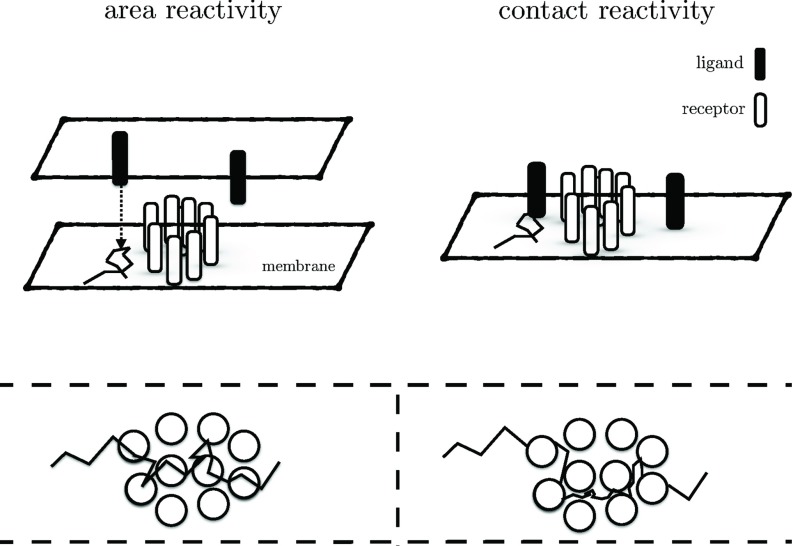
Although we treat only the 2D case, the established general relations between the different quantities remain valid in 1D and 3D, up to some elementary adaptations of the normalization factors. However, the 2D case provides the advantage that exact expressions for the GF solutions both in the Laplace and time domain are known,⁴ meaning that all general relations can be verified explicitly. Moreover, the 2D case is of particular importance for cell-biological applications to facilitate a better understanding of molecular interactions within cell membranes.^3,15 In fact, the CR model may not well reflect the biological reality of certain 2D systems that instead may more accurately depicted by the AR model (Fig. 1). A case in point is the communication between two cells that are in contact. Here, ligands and receptors undergo a diffusive motion on two opposing cell membranes (Fig. 1, top left). In this system, a typical ligand's space-time trajectory may pass through the reaction area and there is a non-vanishing probability to find the ligand unbound within the reaction area (Fig. 1, bottom left). However, such a space-time behavior has no counterpart at all within the CR model, because here the ligands’ trajectories are excluded from the area that is bounded by the encounter radius (Fig. 1, bottom right). Still, the CR model may provide an accurate description for situations where ligands and receptors move on the same cell membrane (Fig. 1, top right).

FIG. 1.

Schematic comparison between the CR and AR model in a cell-biological context. Top left: Ligands and receptors diffuse on opposing membranes of two cells in contact. Bottom left: A typical ligand's trajectory passes through several adjacent reaction areas. Top right: Ligands and receptors undergo diffusive motion on the same cell membrane. Bottom right: Trajectories cannot enter the areas bounded by the encounter radius. Note that, in general, the physical radius of the molecules is not necessarily equal to their encounter radius used in the CR model.

By pointing out similarities and differences between the AR and CR model throughout the paper, we provide further theoretical evidence that the conceptual differences between the two models may indeed lead to significantly different predictions.

II. IRREVERSIBLE REACTION

We consider a pair of molecules A and B that undergo a diffusive motion characterized by diffusion constants D_A and D_B, respectively. Equivalently, one may view this system as a single molecule diffusing with diffusion constant D = D_A + D_B around a static molecule that, without loss of generality, is assumed to be located at the origin. According to the AR model, the molecule may bind whenever its position is located within the static reaction disk of radius r = a. The probability density function (PDF) p(r, t|r₀) gives the likelihood of finding the molecule unbound at a distance r at time t, provided that its distance was initially r₀ at time t = 0. There are two main differences to the CR model. First, the diffusing molecule may be located within the reaction area without being bound, hence, the PDF p(r, t|r₀) is also defined for r < a. Second, the bound state is infinitely degenerate. Therefore, it is natural to introduce another PDF q(r, t|r₀) that gives the probability to find the molecule bound at a distance r at time t, given that it was unbound at a distance r₀ at time zero. The equations of motion of p(r, t|r₀) and q(r, t|r₀) are^3,4

$$\begin{array}{ccc}\hfill \frac{\partial p(r,t|r_0)}{\partial t}& =& {\mathcal{L}}_{r}p(r,t|r_0)-{\kappa }_r\Theta (a-r)p(r,t|r_0),\hfill \end{array}$$ (1)

$$\begin{array}{ccc}\hfill \frac{\partial q(r,t|r_0)}{\partial t}& =& {\kappa }_r\Theta (a-r)p(r,t|r_0),\hfill \end{array}$$ (2)

where Θ(x) denotes the Heaviside step-function that assumes unity for x > 0 and vanishes otherwise. We note that the term κ_rΘ(a − r)p(r, t|r₀) describes the rate of the association reaction and ${\mathcal{L}}_r$ denotes the 2D rotationally symmetric diffusion operator

$${\mathcal{L}}_r=D\frac{1}{r}\frac{\partial }{\partial r}\left(r\frac{\partial }{\partial r}\right).$$ (3)

Equation (1) is referred to as the Feynman-Kac equation. We see that, in the irreversible case, the equations of motion for p(r, t|r₀) and q(r, t|r₀) (Eqs. (1) and (2)) are decoupled and that the equation for the PDF q(r, t|r₀) is an ordinary differential equation.³ In fact, knowledge of p(r, t|r₀) allows to obtain q(r, t|r₀) easily via Eq. (2). The ICs are^3,4

$$\begin{array}{ccc}\hfill p(r,t=0|r_0)& =& \frac{\delta (r-r_0)}{2\pi r_0},\hfill \end{array}$$ (4)

$$\begin{array}{ccc}\hfill q(r,t=0|r_0)& =& 0.\hfill \end{array}$$ (5)

The FKE Eq. (1) is subject to BC at the origin and at infinity,^3,4 respectively,

$$\begin{array}{ccc}\hfill r\frac{\partial }{\partial r}p(r,t|r_0)& & \underset{r\to 0}{\to }0,\hfill \end{array}$$ (6)

$$\begin{array}{ccc}\hfill p(r,t|r_0)& & \underset{r\to \infty }{\to }0.\hfill \end{array}$$ (7)

An important quantity that can be derived from the GF is the survival probability S(t|r₀)

$$S\left(t\right|r_0)=2\pi {\int }_0^{\infty }p(r,t|r_0)rdr$$ (8)

that gives the likelihood that a pair, initially separated by r₀, does not bind by time t. From the IC Eq. (4) it follows that

$$S(t=0|r_0)=1.$$ (9)

It will turn out to be useful to introduce additional survival probabilities S^<(t|r₀), S^>(t|r₀)

$$\begin{array}{c}\hfill S^{<}\left(t\right|r_0):=2\pi {\int }_0^{a}p(r,t|r_0)rdr,\end{array}$$ (10)

$$\begin{array}{c}\hfill S^{>}\left(t\right|r_0):=2\pi {\int }_a^{\infty }p(r,t|r_0)rdr,\end{array}$$ (11)

that give the joint probability that by time t the molecule has not reacted yet and that it is located within/outside the reaction area, respectively, given that it was initially located at a distance r₀. Obviously, one has

$$S\left(t\right|r_0)=S^{<}\left(t\right|r_0)+S^{>}\left(t\right|r_0).$$ (12)

The corresponding IC read

$$\begin{array}{ccc}\hfill S^{<}(t=0|r_0)& =& \Theta (a-r_0),\hfill \end{array}$$ (13)

$$\begin{array}{ccc}\hfill S^{>}(t=0|r_0)& =& \Theta (r_0-a).\hfill \end{array}$$ (14)

Now, by integrating the FKE (Eq. (1)) over all r from the origin to infinity, multiplying by 2π and using the BC Eqs. (6) and (7), we obtain

$$\frac{\partial S\left(t\right|r_0)}{\partial t}=-{\kappa }_r{S}^{<}\left(t\right|r_0).$$ (15)

Note that one may view Eq. (15) as an analogue of the relation that one would find in CR theories

$$\frac{\partial S\left(t\right|r_0)}{\partial t}=-{\kappa }_{a}p(a,t|r_0).$$ (16)

The binding probability is defined by (see Refs. ³ and ⁴)

$$Q\left(t\right|r_0)=2\pi {\int }_0^{\infty }q(r,t|r_0)rdr=2\pi {\int }_0^{a}q(r,t|r_0)rdr,$$ (17)

where the last equation does hold because q(r, t|r₀) = 0 for r > a. For consistency, one requires S(t|r₀) + Q(t|r₀) = 1 for all times. In fact, this follows from the equations of motion, Eqs. (1) and (2), the IC (Eqs. (4) and (5)), and the definitions of the survival and binding probabilities (Eqs. (8) and (17); see also Ref. 4).

The reaction rate gives the fraction of molecule pairs that associate with each other per unit time and is defined by the negative time derivative of the survival probability¹⁴

$$R\left(t\right|r_0)=-\frac{\partial S\left(t\right|r_0)}{\partial t},$$ (18)

which translates to

$$\tilde{R}\left(s\right|r_0)=1-s\tilde{S}\left(s\right|r_0)$$ (19)

in the Laplace domain. In general, we employ the following notation for the Laplace transform of a function f(t)

$$\mathbf{L}\left[f\left(t\right)\right]\left(s\right)=\tilde{f}\left(s\right)={\int }_0^{\infty }{e}^{-st}f\left(t\right)dt.$$ (20)

It follows from Eqs. (15) and (18) that

$$R\left(t\right|r_0)={\kappa }_r{S}^{<}\left(t\right|r_0).$$ (21)

In the context of the classical Smoluchowski theory, one would have the analogous relation¹⁴

$$R\left(t\right|r_0)={\kappa }_{a}p(a,t|r_0),$$ (22)

implying that reactions only take place at contact r = a. The central postulate of the AR model that the reaction may occur throughout an reaction area is reflected in Eq. (21).

To obtain an equation of motion for the survival probability, we start from the FKE Eq. (1), make use of the detailed balance condition

$$p(r,t|r_0)=p(r_0,t|r)$$ (23)

and switch r ↔ r₀, which results in

$$\frac{\partial p(r,t|r_0)}{\partial t}={\mathcal{L}}_{r_0}p(r,t|r_0)-{\kappa }_r\Theta (a-r_0)p(r,t|r_0).$$ (24)

Finally, we integrate Eq. (24) over all space $2\pi {\int }_0^{\infty }rdr$ to arrive at

$$\frac{\partial S\left(t\right|r_0)}{\partial t}={\mathcal{L}}_{r_0}S\left(t\right|r_0)-{\kappa }_r\Theta (a-r_0)S\left(t\right|r_0).$$ (25)

In the same way, again starting from Eq. (24), one can derive that both S^<(t|r₀) and S^>(t|r₀) obey an equation of motion that takes the same form as Eq. (25), but they satisfy different IC (Eqs. (13) and (14)). In this sense, the time evolution of S^<(t|r₀) and S^>(t|r₀) is decoupled.

Now, the Laplace transform of Eq. (25) reads³

$${\mathcal{L}}_{r_0}\tilde{S}\left(s\right|r_0)=[{\kappa }_r\Theta (a-r_0)+s]\tilde{S}\left(s\right|r_0)-1,$$ (26)

which may be rewritten more explicitly as

$${\mathcal{L}}_{r_0}\tilde{S}\left(s\right|r_0)=\left\{\begin{array}{cc}\hfill D{w}^2\tilde{S}\left(s\right|r_0)-1& \hfill \text{if}{r}_0<a,\\ \hfill D{v}^2\tilde{S}\left(s\right|r_0)-1& \hfill \text{if}{r}_0>a,\end{array}\right.$$ (27)

where we defined

$$\begin{array}{ccc}\hfill v& =& \sqrt{\frac{s}{D}},\hfill \end{array}$$ (28)

$$\begin{array}{ccc}\hfill w& =& \sqrt{\frac{s+{\kappa }_r}{D}}.\hfill \end{array}$$ (29)

From Eq. (27) and the Laplace transform of the reaction rate (Eq. (19)), we obtain

$${\mathcal{L}}_{r_0}\tilde{R}\left(s\right|r_0)=\left\{\begin{array}{cc}\hfill D{w}^2\tilde{R}\left(s\right|r_0)-{\kappa }_r& \hfill \text{if}{r}_0<a,\\ \hfill D{v}^2\tilde{R}\left(s\right|r_0)& \hfill \text{if}{r}_0>a.\end{array}\right.$$ (30)

We again note that Eqs. (27) and (30) have counterparts in the classical Smoluchowski theory.¹⁴

Finally, we would like to derive relations between the different survival probabilities S(t|r₀), S^<(t|r₀), S^>(t|r₀). To this end, we start from Eq. (1) to obtain

$$\begin{array}{ccc}\hfill \frac{\partial S^{>}\left(t\right|r_0)}{\partial t}& =& -2\pi aD\frac{\partial p(r,t|r_0)}{\partial r}{|}_{r=a},\hfill \end{array}$$ (31)

$$\begin{array}{ccc}\hfill \frac{\partial S^{<}\left(t\right|r_0)}{\partial t}& =& 2\pi aD\frac{\partial p(r,t|r_0)}{\partial r}{|}_{r=a}-{\kappa }_r{S}^{<}\left(t\right|r_0).\hfill \end{array}$$ (32)

Therefore, we can conclude that

$$S^{>}\left(t\right|r_0)=\Theta (r_0-a)-2\pi aD{\int }_0^t\frac{\partial p(r,\tau |r_0)}{\partial r}{|}_{r=a}d\tau ,$$ (33)

and, using the Laplace transforms of Eqs. (31) and (32), we arrive at

$$\begin{array}{ccc}\hfill {\tilde{S}}^{<}\left(s\right|r_0)& =& \frac{1}{s+{\kappa }_r}-\frac{s}{s+{\kappa }_r}{\tilde{S}}^{>}\left(s\right|r_0),\hfill \end{array}$$ (34)

$$\begin{array}{ccc}\hfill \tilde{S}\left(s\right|r_0)& =& \frac{1}{s+{\kappa }_r}+\frac{{\kappa }_r}{s+{\kappa }_r}{\tilde{S}}^{>}\left(s\right|r_0).\hfill \end{array}$$ (35)

A. Time-dependent rate coefficient

We now turn to the notion of a time-dependent rate coefficient k(t) that plays a central role in the Smoluchowski theory of homogeneous bimolecular reactions.^6–8,16,17 Classically, k(t) is defined as the reactive flux at contact, given an initial equilibrium distribution. Here, we will first seek to relate the reactive flux at contact to quantities that describe an isolated pair, notably the survival probability studied above. Relations of that type have been established for CR theories¹⁴ and we will study how they translate to the AR context. Moreover, by considering more explicitly a many-particle formulation and deriving the macroscopic rate equations for pseudo-first-order reactions, we will show that the usual identification of the rate coefficient as the flux at contact is deficient. In fact, we will conclude that in the AR context an additional term, besides the flux, has to be taken into account that offers a straightforward physical interpretation and vanishes for CR theories.

Following Smoluchowski,^6,8,17 we consider the irreversible reaction A + B → C that is macroscopically described by the rate equation

$$\frac{d\left[A\right]}{dt}=\frac{d\left[B\right]}{dt}=-k\left(t\right)\left[A\right]\left[B\right],$$ (36)

where [A], [B] refer to the global concentrations of A and B, respectively. The central goal of the Smoluchowski theory is to calculate the rate coefficient k(t) from a more microscopic model. To this end, one assumes that the A concentration is so low that it is sufficient to consider a single A molecule that is surrounded by non-self-interacting B reactants, whose distribution around A is microscopically described by the concentration c(r, t). Instead of c(r, t), one frequently considers the reduced concentration, also referred to as radial distribution function of reactants^6,14,17 that is obtained by normalizing c(r, t) to the initial concentration c₀ = [B](t = 0),

$$\rho (r,t|\text{eq})=\frac{c(r,t)}{c_0},$$ (37)

where “eq” indicates that the initial distribution takes the uniform equilibrium form

$$\rho (r,t=0|\text{eq})=\Theta (r-a).$$ (38)

Furthermore, the time evolution of ρ(r, t|eq) is assumed to be governed by the diffusion equation. Then, the time-dependent rate coefficient is defined as the reactive flux at the encounter distance^{6–8,14,16,17}

$$k_{\text{flux}}\left(t\right)=2\pi aD\frac{\partial \rho (r,t|\text{eq})}{\partial r}{|}_{r=a}.$$ (39)

Turning to the AR model, it is not immediately clear that the identification of the rate coefficient, which appears in the rate equation (Eq. (36)), with the flux defined in Eq. (39) is still adequate, because the notion of an encounter radius is abandoned and instead reactions can occur throughout an interaction area. As a prerequisite for addressing this issue, we establish relationships between the flux at the encounter distance and single pair quantities. Henceforth, we use the notation k_flux(t) to refer to the flux, while k_rate(t) refers to the quantity that actually appears in the rate equation. Obviously, one has k_flux(t) = k_rate(t) in the CR model.

To proceed, we exploit that knowledge of the GF p(r, t|r₀) permits calculating the time evolution for any given initial distribution

$$\rho (r,t|\text{eq})=2\pi {\int }_0^{\infty }p(r,t|r_0)\rho (r_0,t=0|\text{eq})r_{0}d{r}_0.$$ (40)

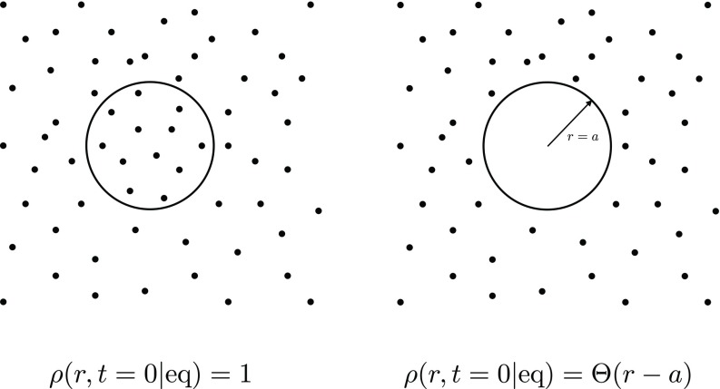
We note that the radial distribution ρ(r, t|eq) satisfies the FKE in the AR model, instead of the diffusion equation. The question arises which initial distribution should be chosen in the present context. Besides the classical choice (Eq. (38)), the following initial distribution now appears as a natural alternative, because molecules may also be located within the reaction area

$$\rho (r,t=0|\text{eq})=1\text{for}\text{all}r,$$ (41)

even for r < a. Note that this choice does not make sense in a CR model. It will be instructive to consider both possibilities, see also Fig. 2 for a schematic representation.

FIG. 2.

Schematic comparison between the two initial distributions used to calculate the rate coefficients $k_{\text{rate}}^{\rho =1}\left(t\right)$ and $k_{\text{rate}}^{\rho =\Theta }\left(t\right)$. The figure on the right represents the choice typically made in the CR model. The figure on the left shows the distribution that appears as a natural alternative to ρ(r, t = 0|eq) = Θ(r − a) within the AR framework.

1. Initial distribution ρ(r, t = 0|eq) = 1

Using the alternative initial condition (Eq. (41)), the detailed balance condition (Eq. (23)) and the definition of the survival probability (Eq. (8)), we see that Eq. (40) implies that the radial distribution of reactants is equal to the survival probability of an isolated pair

$$\rho (r,t|\text{eq})=S(t\left|r\right).$$ (42)

Next, using the definition of the flux Eq. (39) immediately gives

$$k_{\text{flux}}^{\rho =1}\left(t\right)=2\pi aD\frac{\partial S\left(t\right|r_0)}{\partial r_0}{|}_{r_0=a}.$$ (43)

Here and henceforth, we use the superscripts “ρ = 1” and “ρ = Θ” to indicate the corresponding initial distribution. Both relations, Eqs. (42) and (43), are known in analogous form from CR theories.¹⁴ We may now integrate the equation of motion of the survival probability (Eq. (25)) over r₀ from a to ∞ to rewrite Eq. (43) as follows:

$$\begin{array}{ccc}\hfill k_{\text{flux}}^{\rho =1}\left(t\right)& =& -2\pi {\int }_a^{\infty }\frac{\partial S\left(t\right|r_0)}{\partial t}{r}_{0}d{r}_0\hfill \end{array}$$ (44)

$$\begin{array}{ccc}\hfill & =& 2\pi {\int }_a^{\infty }R\left(t\right|r_0)r_{0}d{r}_0,\hfill \end{array}$$ (45)

where the second identity follows from the definition of the reaction rate as the negative time derivative of the survival probability (Eq. (18)). Thus, we have shown that Eq. (43) and hence Eq. (39) is equivalent to Eq. (45). Alternatively, we could have proceeded by using Eqs. (23), (31), and (39)–(41), and the definition of S^>(t|r₀) (Eq. (11)) to write

$$\begin{array}{ccc}\hfill k_{\text{flux}}^{\rho =1}\left(t\right)& =& 4{\pi }^{2}aD{\int }_0^{\infty }\frac{\partial p(r,t|r_0)}{\partial r}{|}_{r=a}{r}_{0}d{r}_0\hfill \end{array}$$ (46)

$$\begin{array}{ccc}& =& -2\pi {\int }_0^{\infty }\frac{\partial S^{>}\left(t\right|r_0)}{\partial t}{r}_{0}d{r}_0\hfill \\ & =& -2\pi {\int }_a^{\infty }\frac{\partial S\left(t\right|r_0)}{\partial t}{r}_{0}d{r}_0.\hfill \end{array}$$ (47)

Furthermore, using Eq. (15) we find that

$$\begin{array}{c}\hfill k_{\text{flux}}^{\rho =1}\left(t\right)={\kappa }_r{S}^{<}\left(t|{\mathbf{B}}_2^C\right)={\kappa }_r{S}^{>}\left(t\right|{\mathbf{B}}_2),\end{array}$$ (48)

where we have introduced

$$\begin{array}{ccc}\hfill S^{<}\left(t|{\mathbf{B}}_2^C\right)& :=& 2\pi {\int }_a^{\infty }{S}^{<}\left(t\right|r_0)r_{0}d{r}_0,\hfill \end{array}$$ (49)

$$\begin{array}{ccc}\hfill S^{>}\left(t\right|{\mathbf{B}}_2)& :=& 2\pi {\int }_0^a{S}^{>}\left(t\right|r_0)r_{0}d{r}_0,\hfill \end{array}$$ (50)

and we also used the definitions Eqs. (10) and (11) to conclude that $S^{<}\left(t\right|{\mathbf{B}}_2^C)=S^{>}\left(t\right|{\mathbf{B}}_2)$. Here B₂ denotes the two dimensional ball of radius a and ${\mathbf{B}}_2^C:={\mathbf{R}}^2\setminus {\mathbf{B}}_2$. Note that $S^{<}\left(t\right|{\mathbf{B}}_2^C)$, S^>(t|B₂) are technically no probabilities, but it is natural to relate these quantities to the probability

$$S^{>}\left(t\right|\text{uni})=\frac{1}{\pi a^2}{S}^{>}\left(t\right|{\mathbf{B}}_2),$$ (51)

that the molecule is found unbound with r > a at time t, given that initially it was uniformly distributed inside the reaction area. Then, we can write

$$\begin{array}{ccc}\hfill k_{\text{flux}}^{\rho =1}\left(t\right)& =& \pi a^2{\kappa }_r{S}^{>}\left(t\right|\text{uni}).\hfill \end{array}$$ (52)

As we have seen, the reactive flux at contact can indeed be related to single pair quantities in a way that is quite reminiscent of the CR case. However, it will turn out that the rate coefficient that appears in the rate equation is not equal to the flux. To see this, we assume that the system of interest is comprised of such a large number of B molecules that it is justified to treat their global concentration as constant [B(t)] = c for all times, i.e., the reaction is pseudo-first-order. Then, within the framework of the CR model it is well-known that the many-particle survival probability $\mathcal{S}\left(t\right|\text{eq})\equiv \left[A\left(t\right)\right]/{\left[A\right]}_0$ can be calculated using the time-dependent rate coefficient via^14,17

$$\mathcal{S}\left(t\right|\text{eq})=e^{-c{\int }_0^t{k}_{\text{rad}}\left(t^{\prime }\right)d{t}^{\prime }},$$ (53)

equivalently, the survival probability $\mathcal{S}\left(t\right|\text{eq})$ satisfies the rate equation

$$\frac{d\mathcal{S}\left(t\right|\text{eq})}{dt}=-c{k}_{\text{rad}}\left(t\right)\mathcal{S}\left(t\right|\text{eq}).$$ (54)

k_rad(t) refers here and henceforth to the rate coefficient in the presence of a radiation BC that plays an important role in the CR model.^7,14,16

To derive Eqs. (53) and (54) within the framework of the AR model, we follow Ref. 17 and first consider a finite system with N copies of B particles. The area and radius of the underlying diffusion space is denoted by $\mathcal{A}$ and $R=\sqrt{\mathcal{A}/\pi }$, respectively. Due to the assumptions discussed above, the many-particle survival probability factorizes¹⁷

$${\mathcal{S}}_N\left(t\right|\text{eq})={\left[2\pi {\int }_0^R\frac{\rho (r,t|\text{eq})}{\mathcal{A}}rdr\right]}^N,$$ (55)

where ρ(r, t|eq) is the radial pair distribution function (Eq. (40)). Taking the time derivative gives

$$\frac{d{\mathcal{S}}_N\left(t\right|\text{eq})}{dt}=\frac{N}{\mathcal{A}}2\pi {\int }_0^R\frac{\partial \rho (r,t|\text{eq})}{\partial t}rdr{\mathcal{S}}_{N-1}\left(t\right|\text{eq}).$$ (56)

Next, we consider the thermodynamic limit, i.e., $N,\mathcal{A}\to \infty$ such that the ratio $N/\mathcal{A}\to c$ remains finite to arrive at

$$\begin{array}{ccc}\hfill \frac{d\mathcal{S}\left(t\right|\text{eq})}{dt}& =& \underset{N,\mathcal{A}\to \infty }{\lim }\frac{d{\mathcal{S}}_N\left(t\right|\text{eq})}{dt}\hfill \\ & =& c2\pi {\int }_0^{\infty }\frac{\partial \rho (r,t|\text{eq})}{\partial t}rdr\mathcal{S}\left(t\right|\text{eq}).\hfill \end{array}$$ (57)

Now, we use Eqs. (25) and (42) to conclude that

$$\begin{array}{c}\hfill 2\pi {\int }_0^{\infty }\frac{\partial \rho (r,t|\text{eq})}{\partial t}rdr=2\pi {\int }_0^{\infty }\frac{\partial S\left(t\right|r)}{\partial t}rdr=-{\kappa }_{r}S\left(t\right|{\mathbf{B}}_2).\end{array}$$ (58)

Thus, we finally arrive at

$$\begin{array}{ccc}\hfill \frac{d{\mathcal{S}}^{\rho =1}\left(t\right|\text{eq})}{dt}& =& -{\kappa }_{r}S\left(t\right|{\mathbf{B}}_2)c{\mathcal{S}}^{\rho =1}\left(t\right|\text{eq}),\hfill \end{array}$$ (59)

$$\begin{array}{ccc}\hfill {\mathcal{S}}^{\rho =1}\left(t\right|\text{eq})& =& \exp \left[-c{\kappa }_r{\int }_0^{t}S\left(t^{\prime }\right|{\mathbf{B}}_2)d{t}^{\prime }\right].\hfill \end{array}$$ (60)

Note that we here use again the superscript “ρ = 1” to indicate the initial distribution. We can now read off the “true” rate coefficient from Eq. (59)

$$\begin{array}{ccc}\hfill k_{\text{rate}}^{\rho =1}\left(t\right)& =& {\kappa }_{r}S\left(t\right|{\mathbf{B}}_2)\hfill \\ \\ & \ne & k_{\text{flux}}^{\rho =1}\left(t\right),\hfill \end{array}$$ (61)

see Eq. (48). We find that the classical definition of the rate coefficient as the reactive flux has to be modified. From S(t|B₂) = S^>(t|B₂) + S^<(t|B₂) and Eqs. (48), (15), and (42) we can infer how the definition of the rate coefficient has to be changed to obtain Eq. (61)

$$\begin{array}{ccc}\hfill k_{\text{rate}}^{\rho =1}\left(t\right)& =& k_{\text{flux}}^{\rho =1}\left(t\right)-2\pi \frac{\partial }{\partial t}{\int }_0^a\rho (r,t|\text{eq})rdr\hfill \end{array}$$ (62)

$$\begin{array}{ccc}& =& 2\pi {\kappa }_r{\int }_0^a\rho (r,t|\text{eq})rdr.\hfill \end{array}$$ (63)

From a physical point of view, this definition of the rate coefficient can be interpreted readily: It reflects that the rate of the reaction is not only determined by the reactive flux at the encounter distance but also by the reaction rate of the B molecules inside the reaction area. Clearly, for CR theories, the second term in Eq. (62) always vanishes and one recovers the classical result k_rate = k_flux. As a consequence of Eq. (62), we obtain

$$k_{\text{rate}}^{\rho =1}\left(t\right)=-2\pi {\int }_0^{\infty }\frac{\partial }{\partial t}S\left(t\right|r)rdr=2\pi {\int }_0^{\infty }R\left(t\right|r)rdr,$$ (64)

where we also used Eqs. (42) and (44). Let us finally point out that in the CR case, due to the radiation BC, k_rad(t) is also related to the single pair survival probability at contact¹⁴

$$k_{\text{rad}}\left(t\right)={\kappa }_{a}S\left(t\right|a),$$ (65)

again resembling the AR result (Eq. (61)) that we obtained.

2. Initial distribution ρ(r, t = 0|eq) = Θ(r − a)

We now consider the classical choice for the initial distribution (Eq. (38)). We can proceed similar to the case ρ(r, t = 0|eq) = 1 and hence present only the results. We obtain

$$\begin{array}{ccc}\hfill \rho (r,t|\text{eq})& =& S^{>}\left(t\right|r_0),\hfill \end{array}$$ (66)

$$\begin{array}{ccc}& & k_{\text{flux}}^{\rho =\Theta }\left(t\right)=2\pi aD\frac{\partial S^{>}\left(t\right|r_0)}{\partial r_0}{|}_{r_0=a}\hfill \end{array}$$ (67)

$$\begin{array}{ccc}& =& -2\pi {\int }_a^{\infty }\frac{\partial S^{>}\left(t\right|r)}{\partial t}rdr\hfill \\ & =& \frac{\partial S^{>}\left(t\right|{\mathbf{B}}_2)}{\partial t}+S^{>}\left(t\right|{\mathbf{B}}_2).\hfill \end{array}$$ (68)

Again, by deriving the macroscopic rate equations for the pseudo-first-order reaction, we conclude that the rate coefficient is not equal to the flux, but instead the definition Eq. (62) has to be used to obtain

$$\begin{array}{ccc}\hfill {\mathcal{S}}^{\rho =\Theta }\left(t\right|\text{eq})& =& e^{-c{\int }_0^t{k}_{\text{rate}}^{\rho =\Theta }\left(t^{\prime }\right)d{t}^{\prime }},\hfill \end{array}$$ (69)

$$\begin{array}{ccc}\hfill k_{\text{rate}}^{\rho =\Theta }\left(t\right)& =& {\kappa }_r{S}^{>}\left(t\right|{\mathbf{B}}_2).\hfill \end{array}$$ (70)

We note that

$$k_{\text{flux}}^{\rho =1}\left(t\right)=k_{\text{rate}}^{\rho =\Theta }\left(t\right).$$ (71)

B. Numerical construction of the many-particle survival probability

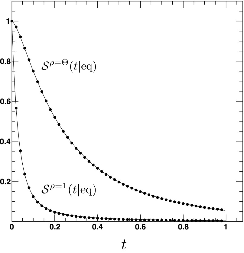
We performed Brownian Dynamics simulations to test the validity of the theoretical considerations and of the results that finally led to the expressions for the many-particle survival probabilities ${\mathcal{S}}^{\rho =1}\left(t\right|\text{eq}),{\mathcal{S}}^{\rho =\Theta }\left(t\right|\text{eq})$ (Eqs. (60) and (69)) in terms of the rate coefficients $k_{\text{rate}}^{\rho =1}\left(t\right),k_{\text{rate}}^{\rho =\Theta }\left(t\right)$. To this end, we considered the irreversible binding reaction A + B → C and chose the following simulation set up: A single molecule A was placed at the origin of the simulation area and held fixed during the simulation. N = 100 copies of B molecules were uniformly distributed throughout the simulation area $\mathcal{A}=L^2$ either including or excluding the reaction area, corresponding to the initial distributions shown in Fig. 2. The B molecules were allowed to diffuse with diffusion constant D and periodic boundary conditions were applied at the system boundaries. Whenever a B molecule's position was inside the reaction area before and after a time step (at t_i and t_i + Δt), a binding reaction took place with probability κ_rΔt. When a binding occurred, the corresponding reaction time t_reac was recorded, the simulation run stopped, and another run for the re-initialized system started. When there was no reaction during t_sim = 1, the reaction time t_reac = t_sim was recorded. We performed 10⁵ simulation runs and calculated for the time points n · 0.01, n = 0 …99 the fraction of reaction times that satisfy t_reac > n · 0.01. The result is shown in Fig. 3. Note that we used the exact expressions for the rate coefficients $k_{\text{rate}}^{\rho =1}\left(t\right),k_{\text{rate}}^{\rho =\Theta }\left(t\right)$ (Eqs. (A1) and (A3)) to calculate the many-particle survival probabilities ${\mathcal{S}}^{\rho =1}\left(t\right|\text{eq}),{\mathcal{S}}^{\rho =\Theta }\left(t\right|\text{eq})$ according to Eqs. (60) and (69), respectively. We find excellent agreement between analytical and simulation results.

FIG. 3.

The many-particle survival probabilities ${\mathcal{S}}^{\rho =1}\left(t\right|\text{eq}),{\mathcal{S}}^{\rho =\Theta }\left(t\right|\text{eq})$ corresponding to the two different initial conditions (Eqs. (41) and (38) respectively). The chosen parameters are D = 0.25, a = 1, κ_r = 10, a = 1, L = 10. The solid lines refer to the analytical expressions (Eqs. (60) and (69)), the markers indicate the simulation results.

C. Asymptotic and approximate expressions for the rate coefficient

1. Short-time expansion

To derive a short time asymptotic expansion of $k_{\text{rate}}^{\rho =1}\left(t\right)$, we use Eqs. (42) and (62) as well as Eqs. (35), (36), (40), and (43) from Ref. 4 and switch to the Laplace domain

$$\begin{array}{ccc}\hfill {\tilde{k}}_{\text{rate}}^{\rho =1}\left(s\right)& =& 2\pi {\kappa }_r{\int }_0^a\tilde{S}\left(s\right|r)rdr=\frac{\pi a^2{\kappa }_r}{s}-\frac{\pi a^2{\kappa }_r^2}{Ds{w}^2}\hfill \\ & & +\frac{2\pi {\kappa }_r^{2}va}{Ds{w}^3}\frac{K_1\left(va\right)I_1\left(wa\right)}{\mathcal{N}},\hfill \end{array}$$ (72)

where

$$\mathcal{N}=v{I}_0\left(wa\right)K_1\left(va\right)+w{I}_1\left(wa\right)K_0\left(va\right)$$ (73)

and v and w are defined by Eqs. (28) and (29), respectively. Because t → 0 corresponds to s → ∞ in the Laplace domain, we can expand the first two terms on the rhs of Eq. (72) as

$$\frac{\pi a^2{\kappa }_r}{s}-\frac{\pi a^2{\kappa }_r^2}{Ds{w}^2}=\frac{\pi a^2{\kappa }_r}{s}\left[1-\frac{{\kappa }_r}{s}+\frac{{\kappa }_r^2}{s^2}+...\right],$$ (74)

where we used $w=v\sqrt{1+{\kappa }_r/s}$. Making use of the large argument expansions of the modified Bessel functions (Appendix III, Eqs. (11) and (12) in Ref. 18), we obtain for the third term on the rhs of Eq. (72)

$$\begin{array}{ccc}& & \frac{2\pi {\kappa }_r^{2}va}{Ds{w}^3}\frac{K_1\left(va\right)I_1\left(wa\right)}{\mathcal{N}}\hfill \\ & & =\frac{\pi a\sqrt{D}{\kappa }_r^2}{s^{\frac{5}{2}}}\left[1-\left(\frac{3}{8}\frac{D}{a^2}+\frac{7}{4}{\kappa }_r\right)\frac{1}{s}+...\right].\hfill \end{array}$$ (75)

To convert these expressions to their time domain counterpart, we employ (Appendix V, Eq. (2) in Ref. 18)

$${\mathbf{L}}^{-1}\left(\frac{1}{s^{\nu +1}}\right)=\frac{t^{\nu }}{\Gamma (\nu +1)}.$$ (76)

Using $\Gamma (5/2)=3/4\sqrt{\pi },\Gamma (7/2)=15/8\sqrt{\pi }$, we arrive at

$$\begin{array}{ccc}\hfill k_{\text{rate}}^{\rho =1}\left(t\right)& =& \pi a^2{\kappa }_r\left[1-{\kappa }_{r}t+\frac{{\kappa }_r^2{t}^2}{2}+...\right]\hfill \\ & & +{\kappa }_r^2\sqrt{\pi D{a}^2{t}^3}\left[\frac{4}{3}-\left(\frac{1}{5}\frac{D}{a^2}+\frac{14}{15}{\kappa }_r\right)t+...\right].\hfill \end{array}$$ (77)

We now turn to the short-time expansion of $k_{\text{rate}}^{\rho =\Theta }\left(t\right)$. We can proceed along the same lines detailed for $k_{\text{rate}}^{\rho =\Theta }\left(t\right)$ above, hence we give only the results. In the Laplace domain, we find

$$\begin{array}{ccc}\hfill {\tilde{k}}_{\text{rate}}^{\rho =\Theta }\left(s\right)& =& \frac{2\pi a{\kappa }_r}{Dvw}\frac{K_1\left(va\right)I_1\left(wa\right)}{\mathcal{N}}\hfill \\ & =& \pi a{\kappa }_r\sqrt{D}\frac{1}{s^{3/2}}\left[1-\left(\frac{3}{8}\frac{D}{a^2}+\frac{3}{4}{\kappa }_r\right)\frac{1}{s}+...\right],\hfill \end{array}$$ (78)

which leads us to

$$k_{\text{rate}}^{\rho =\Theta }\left(t\right)=\sqrt{4\pi Dt}a{\kappa }_r\left[1-\frac{1}{2}\left(\frac{1}{2}\frac{D}{a^2}+{\kappa }_r\right)t+...\right].$$ (79)

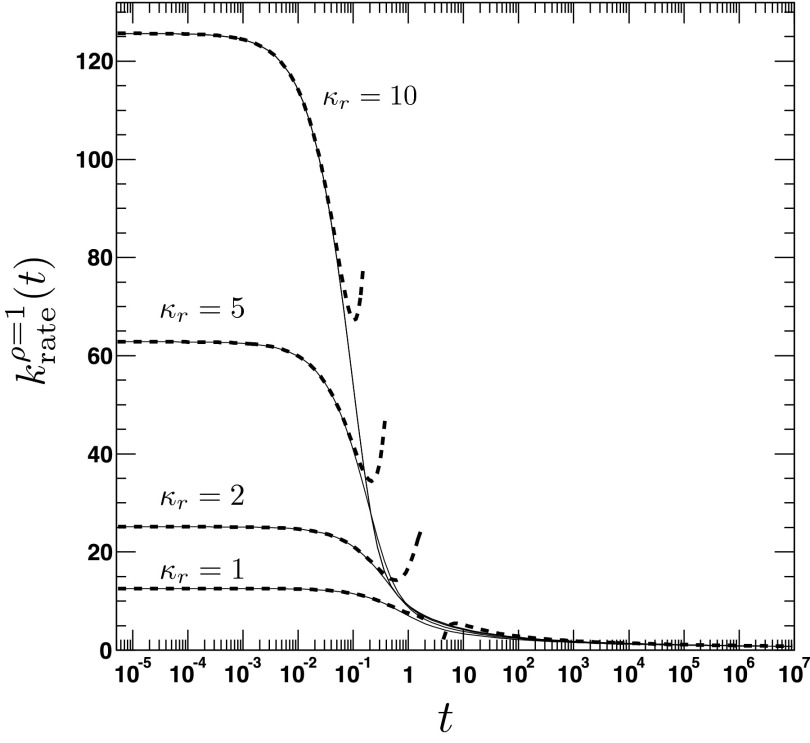
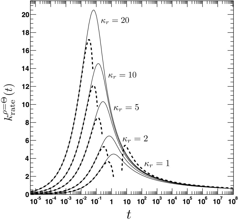
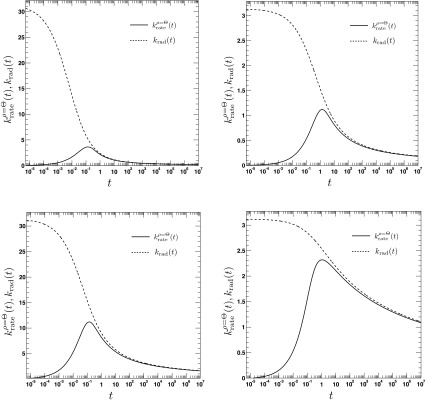
We compare the obtained small-time expansions (Eqs. (77) and (79)) with the exact expressions of $k_{\text{rate}}^{\rho =1}\left(t\right)$ and $k_{\text{rate}}^{\rho =\Theta }\left(t\right)$ (Eqs. (A1) and (A3)) for various values of κ_r. The results are shown in Figs. 4 and 5. We find excellent agreement for sufficiently small times. In addition, Figs. 4 and 5 show that the transient behaviors of $k_{\mathrm{rate}}^{\rho =1}\left(t\right)$ and $k_{\mathrm{rate}}^{\rho =\Theta }\left(t\right)$ significantly differ from each other. The physical origin for this difference is clearly reflected in Eqs. (77) and (79). We note that $k_{\text{rate}}^{\rho =1}\left(t\right)$ is comprised of two distinct groups of terms. Terms that scale like powers of t with integer exponents do not include the diffusion constant D and describe the depletion of molecules that are inside the reaction area initially. Hence, even in the limiting case D → 0 these terms contribute to $k_{\text{rate}}^{\rho =1}\left(t\right)$ and lead to a non-vanishing rate coefficient at t = 0. We point out that this group of terms arises from the second term Eq. (62). The second group of terms scale like powers of t with fractional exponents and take into account the supply of fresh molecules that enter the reaction area due to their diffusive motion, therefore these terms vanish for D → 0. In contrast to $k_{\text{rate}}^{\rho =1}\left(t\right)$, the rate coefficient $k_{\text{rate}}^{\rho =\Theta }\left(t\right)$ exhibits nonmonotonic behavior. In particular, it vanishes at t = 0, because, initially, no molecules are located within the reaction area. The short-time expansion of $k_{\text{rate}}^{\rho =\Theta }\left(t\right)$ solely contains terms that scale like powers of t with fractional exponents and that vanish for D → 0, indicating that only when the outside molecules diffuse into the reaction area depletion can start and $k_{\text{rate}}^{\rho =\Theta }\left(t\right)$ increases. Finally, it is instructive to compare the obtained expressions (Eqs. (77) and (79)) with the CR results for absorbing and radiation BC,¹⁹ respectively,

$$\begin{array}{ccc}\hfill k_{\text{abs}}\left(t\right)& =& 2\pi D\left[\frac{1}{\sqrt{\pi \tau }}+\frac{1}{2}-\frac{1}{4}\sqrt{\frac{\tau }{\pi }}+...\right],\hfill \end{array}$$ (80)

$$\begin{array}{ccc}\hfill k_{\text{rad}}\left(t\right)& =& {\kappa }_a\left[1-2\tilde{h}\sqrt{\frac{\tau }{\pi }}+\tilde{h}\left(\tilde{h}+\frac{1}{2}\right)\tau +...\right],\hfill \end{array}$$ (81)

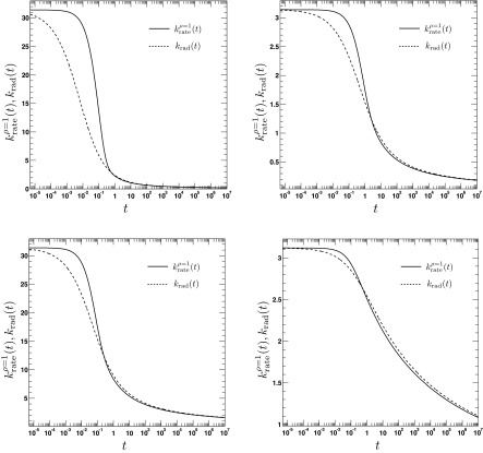
where τ = D/a²t, $\tilde{h}={\kappa }_a/\left(2\pi D\right)$. We emphasize the following points. First, the AR model, given that ρ(r, t = 0|eq) = Θ(r − a), predicts a rate coefficient that does not possess a singularity at t = 0, similar to the CR model with radiation BC, but in contrast to the case of absorbing BC. Second, $k_{\text{rate}}^{\rho =\Theta }\left(t\right)$ vanishes at t = 0, whereas the CR model with radiation BC gives k_rad(t = 0) = κ_a. Third, it follows from Eqs. (79) and (81) that ${\int }_0^t{k}_{\text{rate}}^{\rho =\Theta }\left(\tau \right)d\tau \sim t^{3/2},{\int }_0^t{k}_{\text{rad}}\left(\tau \right)d\tau \sim t$, which implies that for small times the time integral over the time-dependent rate coefficient grows slower in the AR case than in the CR case. The significant differences between the alternate expressions for the rate coefficient are evident in Fig. 6, where the time evolution of $k_{\text{rate}\left(t\right)}^{\rho =\Theta }$ is compared to its classical counterpart k_rad(t)¹⁶ for several values of κ_r and D. In contrast to $k_{\text{rate}}^{\rho =\Theta }\left(t\right)$, the rate coefficient associated with ρ(r, t = 0|eq) = 1 gives $k_{\text{rate}}^{\rho =1}(t=0)=\pi a^2{\kappa }_r$, similar to k_rad(t), see Fig. 7. Still, it is significantly different from k_rad(t), for instance, the next leading order term scales like t, instead of t^1/2, and does not contain the diffusion constant D.

FIG. 4.

The time-dependent rate coefficient for the irreversible reaction, given the initial distribution ρ(r, t = 0|eq) = 1. The figure shows the time dependence of the rate coefficient $k_{\text{rate}}^{\rho =1}\left(t\right)$ for various values of the association constant κ_r = 1, 2, 5, 10. The other parameters are D = 1, a = 2. The solid lines are obtained from the analytical expression for $k_{\text{rate}}^{\rho =1}\left(t\right)$ (Eq. (A1)). The dashed lines refer to the approximate solutions for short (Eq. (77)) and long times (Eq. (85)).

FIG. 5.

The time-dependent rate coefficient for the irreversible reaction, given the initial distribution ρ(r, t = 0|eq) = Θ(r − a). The figure shows the time dependence of the rate coefficient $k_{\text{rate}}^{\rho =\Theta }\left(t\right)$ for various values of the association constant κ_r = 1, 2, 5, 10, 20. The other parameters are D = 1, a = 2. The solid lines are obtained from the analytical expression for $k_{\text{rate}}^{\rho =\Theta }\left(t\right)$ (Eq. (A3)). The dashed lines refer to the approximate solutions for short (Eq. (79)) and long times (Eq. (85)).

FIG. 6.

The time dependence of the irreversible rate coefficients $k_{\text{rate}}^{\rho =\Theta }\left(t\right),k_{\text{rad}}\left(t\right)$ according to the area (solid lines, Eq. (A3)) and contact reactivity model¹⁶ (dashed lines), respectively. The encounter radius is a = 1. The other parameters are for the top left panel: κ_r = 10, D = 0.25, top right panel: κ_r = 1, D = 0.25, bottom left panel: κ_r = 10, D = 2.5, bottom right panel: κ_r = 1, D = 2.5. To relate the parameters κ_a and κ_r, we set κ_a = πa²κ_r.

FIG. 7.

The time dependence of the irreversible rate coefficients $k_{\text{rate}}^{\rho =1}\left(t\right),k_{\text{rad}}\left(t\right)$ according to the area (Eq. (A1), solid lines) and contact reactivity model¹⁶ (dashed lines), respectively. The encounter radius is a = 1. The other parameters are for the top left panel: κ_r = 10, D = 0.25, top right panel: κ_r = 1, D = 0.25, bottom left panel: κ_r = 10, D = 2.5, bottom right panel: κ_r = 1, D = 2.5. To relate the parameters κ_a and κ_r, we set κ_a = πa²κ_r.

2. Long-time expansion

We are now interested in $k_{\text{rate}}^{\rho =1},k_{\text{rate}}^{\rho =\Theta }$ for long times t → ∞. Because of Eqs. (35), (61), and (70), we can immediately conclude that both rate coefficients asymptotically exhibit the same long-time behavior. Therefore, we will drop the superscripts “ρ = 1” and “ρ = Θ” in this subsection. Using Eq. (78) as a starting point and the small-argument expansion of the modified Bessel functions (Appendix III, Eqs. (7) and (10) in Ref. 18), we arrive at

$${\tilde{k}}_{\text{rate}}\left(s\right)=-4\pi D\frac{1}{s\ln \left(\frac{1}{4D}{a}^2{e}^{2(\gamma -\rho )}s\right)},$$ (82)

where γ = 0.577216… denotes the Euler-Mascheroni constant (Eq. (6.1.3) in Ref. 20) and

$$\rho =\frac{I_0\left(\sqrt{{\kappa }_r/D}a\right)}{I_1\left(\sqrt{{\kappa }_r/D}a\right)}\sqrt{\frac{D}{a^2{\kappa }_r}}.$$ (83)

For the inversion to the time domain, we employ¹⁹

$$-{\mathbf{L}}^{-1}\left[\frac{1}{s\ln \left(Cs\right)}\right]=\frac{1}{\ln \left(C^{-1}t\right)}-\frac{\gamma }{{\left(\ln C^{-1}t\right)}^2}+...,$$ (84)

where C > 0 denotes an arbitrary constant to obtain finally

$$\begin{array}{ccc}\hfill k_{\text{rate}}\left(t\right)& =& 4\pi D(\frac{1}{\ln \left(4\tau \right)-2\gamma +2\rho }\hfill \\ & & -\frac{\gamma }{{[\ln \left(4\tau \right)-2\gamma +2\rho ]}^2}+...),\hfill \end{array}$$ (85)

that is quite similar to the corresponding expansion within the framework of the CR model.¹⁹

III. REVERSIBLE REACTIONS

For the reversible reaction, the equations of motion of the PDF p_rev(r, t|r₀) and q_rev(r, t|r₀) need to be extended to allow for dissociation of the bound pair³

$$\begin{array}{ccc}\hfill \frac{\partial p_{\text{rev}}(r,t|r_0)}{\partial t}& =& {\mathcal{L}}_r{p}_{\text{rev}}(r,t|r_0)-{\kappa }_r\Theta (a-r)p_{\text{rev}}(r,t|r_0)\hfill \\ & & +{\kappa }_d{q}_{\text{rev}}(r,t|r_0),\hfill \end{array}$$ (86)

$$\begin{array}{ccc}\hfill \frac{\partial q_{\text{rev}}(r,t|r_0)}{\partial t}& =& {\kappa }_r\Theta (a-r)p_{\text{rev}}(r,t|r_0)-{\kappa }_d{q}_{\text{rev}}(r,t|r_0).\hfill \end{array}$$ (87)

Note that the equations of motion are now coupled, in contrast to their irreversible cousins, due to the appearance of the term κ_dq_rev(r, t|r₀), which yields the rate of dissociation.³ Obviously, Eqs. (86) and (87) reduce to their irreversible counterparts Eqs. (1) and (2) for κ_d → 0. p_rev(r, t|r₀) is subject to the same BC at the origin and at infinity as its irreversible analogue (Eqs. (6) and (7)). Regarding the IC, we have to be aware of the fact that for the reversible reaction also the bound pair represents a possible initial state. Therefore, besides the IC that describe the initially unbound molecule (Eqs. (4) and (5)), we have to include in our description the following set of IC:³

$$\begin{array}{ccc}\hfill p_{\text{rev}}(r,t|r_0,*)& =& 0,\hfill \end{array}$$ (88)

$$\begin{array}{ccc}\hfill q_{\text{rev}}(r,t|r_0,*)& =& \frac{\delta (r-r_0)}{2\pi r_0}.\hfill \end{array}$$ (89)

Here, we make use of the notation adopted in Ref. 4, where the initially bound state is indicated by the symbol * and the corresponding quantities like the GF solutions, etc., are denoted by p_rev(r, t|r₀, *), q_rev(r, t|r₀, *), and so forth.

Survival as well as binding probabilities and the reaction rate are technically defined in the same manner as in the irreversible case (Eqs. (8), (10), (11), (17), and (18)). However, we would like to point out that in the context of the reversible reaction the term “survival probability” is conceptually somewhat misleading. Instead, the term “separation probability”¹⁴ provides a more accurate description, because being unbound at time t does not necessarily imply that the molecule was not bound before t and dissociated again, in contrast to the irreversible case.^12,14 Nevertheless, the notion “survival probability” is also still widely used in the context of the reversible reaction.¹¹ We adhere to this tradition and shall use both terms interchangeably.

A. Initially unbound state

Next, we aim at finding an expression for the reaction rate R_rev(t|r₀) in terms of $S_{\text{rev}}^{<}\left(t\right|r_0)$. To this end, we integrate Eq. (86) over all space, multiply the equation by 2π, and thus obtain

$$\frac{\partial S_{\text{rev}}\left(t\right|r_0)}{\partial t}=-{\kappa }_r{S}_{\text{rev}}^{<}\left(t\right|r_0)+{\kappa }_d[1-S_{\text{rev}}\left(t\right|r_0)].$$ (90)

The Laplace transform of this equation may be rewritten by virtue of the relation (19), which remains valid in the reversible case, provided that one considers the initially unbound molecule. Thus, the reaction rate in the Laplace domain turns out to be

$${\tilde{R}}_{\text{rev}}\left(s\right|r_0)=\frac{{\kappa }_{r}s}{s+{\kappa }_d}{\tilde{S}}_{\text{rev}}^{<}\left(s\right|r_0).$$ (91)

We observe that Eq. (91) assumes the same structure as its irreversible counterpart (Eq. (21)). In fact, the sole difference lies in the form of the recombination rate κ_rs/(s + κ_d) that becomes dependent from s in the reversible case. In the limit κ_d → 0, the recombination rate reduces to κ_r, as it should. This is quite reminiscent of the situation in the CR model, see Ref. 14, Eq. (3.3b).

We now turn to the equation of motion for the survival probability that may be derived by applying the same procedure we already used in Sec. II. However, we have to be aware of the fact that in general

$$q(r,t|r_0)\ne q(r_0,t|r).$$ (92)

This issue can easily be dealt with by solving Eq. (87) and expressing q_rev(r, t|r₀) in terms of p_rev(r, t|r₀)

$$q_{\text{rev}}(r,t|r_0)={\kappa }_r\Theta (a-r){\int }_0^t{e}^{-{\kappa }_d(t-t^{\prime })}{p}_{\text{rev}}(r,t^{\prime }|r_0)d{t}^{\prime },$$ (93)

where we also used the IC q(r, t = 0|r₀) = 0. Then, employing the detailed balance condition (Eq. (23)) and interchanging r ↔ r₀, we find

$$\begin{array}{ccc}\hfill \frac{\partial p_{\text{rev}}(r,t|r_0)}{\partial t}& =& {\mathcal{L}}_{r_0}{p}_{\text{rev}}(r,t|r_0)\hfill \\ & & -{\kappa }_r\Theta (a-r_0)[p_{\text{rev}}(r,t|r_0)\hfill \\ & & -{\kappa }_d{\int }_0^t{e}^{-{\kappa }_d(t-t^{\prime })}{p}_{\text{rev}}(r,t^{\prime }|r_0)d{t}^{\prime }].\hfill \end{array}$$ (94)

We integrate over all space to arrive at

$$\begin{array}{ccc}\hfill \frac{\partial S_{\text{rev}}\left(t\right|r_0)}{\partial t}& =& {\mathcal{L}}_{r_0}{S}_{\text{rev}}\left(t\right|r_0)\hfill \\ & & -{\kappa }_r\Theta (a-r_0)[S_{\text{rev}}\left(t\right|r_0)\hfill \\ & & -{\kappa }_d{\int }_0^t{e}^{-{\kappa }_d(t-t^{\prime })}{S}_{\text{rev}}\left(t^{\prime }\right|r_0)d{t}^{\prime }].\hfill \end{array}$$ (95)

We point out that, as in the irreversible case, one can demonstrate by virtue of Eq. (94) that both $S_{\text{rev}}^{<}\left(t\right|r_0)$ and $S_{\text{rev}}^{>}\left(t\right|r_0)$ obey the same equation of motion as S_rev(t|r₀) (Eq. (95)) and that again they are subject to different IC, cf. Eqs. (13) and (14). Next, the Laplace transform of Eq. (95) yields³

$$s{\tilde{S}}_{\text{rev}}\left(s\right|r_0)-1={\mathcal{L}}_{r_0}{\tilde{S}}_{\text{rev}}\left(s\right|r_0)-\frac{{\kappa }_{r}s}{s+{\kappa }_d}\Theta (a-r_0){\tilde{S}}_{\text{rev}}\left(s\right|r_0).$$ (96)

We note that Eq. (96) enjoys exactly the same form as its irreversible counterpart, provided one makes the by now obligatory substitution κ_r → κ_rs/(s + κ_d). Equation (96) may be rewritten as

$${\mathcal{L}}_{r_0}{\tilde{S}}_{\text{rev}}\left(s\right|r_0)=\left\{\begin{array}{cc}\hfill D{w}^2{\tilde{S}}_{\text{rev}}\left(s\right|r_0)-1& \hfill \text{if}{r}_0<a\\ \hfill D{v}^2{\tilde{S}}_{\text{rev}}\left(s\right|r_0)-1& \hfill \text{if}{r}_0>a,\end{array}\right.$$ (97)

where w is now defined by

$$\begin{array}{ccc}\hfill w& =& v\sqrt{\frac{s+{\kappa }_r+{\kappa }_d}{s+{\kappa }_d}}.\hfill \end{array}$$ (98)

Obviously, w reduces to the corresponding irreversible expressions Eq. (29) for κ_d = 0. By appeal of Eq. (19), the relation for the reaction rate becomes

$${\mathcal{L}}_{r_0}{\tilde{R}}_{\text{rev}}\left(s\right|r_0)=\left\{\begin{array}{cc}\hfill D{w}^2{\tilde{R}}_{\text{rev}}\left(s\right|r_0)-\frac{{\kappa }_{r}s}{s+{\kappa }_d}& \hfill \text{if}{r}_0<a\\ \hfill D{v}^2{\tilde{R}}_{\text{rev}}\left(s\right|r_0)& \hfill \text{if}{r}_0>a.\end{array}\right.$$ (99)

Note that Eq. (99) could alternatively have been obtained by Eq. (30) via the standard replacement κ_r → κ_rs/(s + κ_d).

Finally, we show how S_rev(t|r₀) relates to $S_{\text{rev}}^{>}\left(t\right|r_0)$. Laplace-transforming Eq. (90), we obtain

$${\tilde{S}}_{\text{rev}}\left(s\right|r_0)=\frac{s+{\kappa }_d}{s(s+{\kappa }_r+{\kappa }_d)}+\frac{{\kappa }_r}{s+{\kappa }_r+{\kappa }_d}{\tilde{S}}_{\text{rev}}^{>}\left(s\right|r_0),$$ (100)

generalizing the relation for the irreversible reaction (Eq. (35)) to the reversible case. Again, alternatively, Eq. (100) would follow from the irreversible relation (35) by substituting κ_r → κ_rs/(s + κ_d).

B. Reversible time-dependent rate coefficient

To give meaning to the notion of the reversible time-dependent rate coefficient within the framework, we can proceed in analogy to the irreversible case. Here, we only consider the initial distribution ρ(r, t = 0|eq) = 1, if not explicitly stated otherwise, and hence we will drop the superscript “ρ = 1” in the following. Note that the case of ρ(r, t = 0|eq) = Θ(r − a) can be treated similarly.

Using the definition Eq. (62) as well as Eq. (42), one can show that Eq. (64) remains valid in exactly the same form for the irreversible as well as reversible reaction within the AR framework, the only necessary replacements consist of straightforward switching k_rate(t) → k_rev(t), S(t|r₀) → S_rev(t|r₀).

We should keep in mind that it is also possible to relate k_rev(t) to the survival probability at contact¹⁴ (Eq. (3.5)) within the framework of the CR model

$${\tilde{k}}_{\text{rev}}\left(s\right)=\frac{s{\kappa }_a}{s+{\kappa }_d}{\tilde{S}}_{\text{rev}}\left(s\right|a).$$ (101)

Analogously, we find

$${\tilde{k}}_{\text{rev}}\left(s\right)=\frac{s{\kappa }_r}{s+{\kappa }_d}{\tilde{S}}_{\text{rev}}\left(s\right|{\mathbf{B}}_2),$$ (102)

where we used Eqs. (64) and (90). As already pointed out in Sec. II, the quantity S_rev(t|B₂) does not technically represent probabilities. However, it is again possible to relate this quantity to the probability

$$S_{\text{rev}}\left(t\right|\text{uni})=\frac{1}{\pi a^2}{S}_{\text{rev}}\left(t\right|{\mathbf{B}}_2),$$ (103)

that the molecule is found unbound at time t, given that initially it was uniformly distributed inside the reaction area. Hence, we may write

$$\begin{array}{c}\hfill {\tilde{k}}_{\text{rev}}\left(s\right)=\frac{s\pi a^2{\kappa }_r}{s+{\kappa }_d}{\tilde{S}}_{\text{rev}}\left(s\right|\text{uni}).\end{array}$$ (104)

We will later employ this relation to give a simple proof that ${\int }_0^{\infty }{k}_{\text{rev}}\left(t\right)dt=K_{\text{eq}}$.

C. Initially bound state

We now focus on the initially bound state. One can show that the GF solutions corresponding to the initially bound and unbound state are related by^3,4

$${\tilde{p}}_{\text{rev}}(r,s|r_0,*)=\frac{{\kappa }_d}{s+{\kappa }_d}{\tilde{p}}_{\text{rev}}(r,s|r_0).$$ (105)

It follows immediately that

$$\begin{array}{c}\hfill {\tilde{S}}_{\text{rev}}\left(s\right|r_0,*)=\frac{{\kappa }_d}{s+{\kappa }_d}{\tilde{S}}_{\text{rev}}\left(s\right|r_0).\end{array}$$ (106)

A similar relation between the separation probabilities of the two IC (bound and unbound state) is well-known from CR models,¹⁴ (Eq. (3.15) and leads to a convolution relation in the time domain

$$S_{\text{rev}}\left(t\right|r_0,*)={\kappa }_d{\int }_0^t{e}^{-{\kappa }_d(t-t^{\prime })}{S}_{\text{rev}}\left(t^{\prime }\right|r_0)d{t}^{\prime }.$$ (107)

We now express ${\tilde{S}}_{\text{rev}}\left(s\right|r_0)$ by ${\tilde{S}}_{\text{rev}}\left(s\right|r_0,*)$ via Eq. (106) and insert the result in Eq. (104) to obtain

$$\begin{array}{c}\hfill {\tilde{k}}_{\text{rev}}\left(s\right)=\frac{s\pi a^2{\kappa }_r}{{\kappa }_d}\tilde{S}\left(s\right|\text{uni},*).\end{array}$$ (108)

Because S(t = 0| uni, *) = 0, this relation yields in the time domain

$$\begin{array}{c}\hfill k_{\text{rev}}\left(t\right)=\frac{\pi a^2{\kappa }_r}{{\kappa }_d}\frac{\partial }{\partial t}S\left(t\right|\text{uni},*).\end{array}$$ (109)

Hence, we can easily conclude that

$${\int }_0^{\infty }{k}_{\text{rev}}\left(t\right)dt=\frac{\pi a^2{\kappa }_r}{{\kappa }_d}=K_{\text{eq}},$$ (110)

see Refs. ⁴ and ¹⁴. Finally, we consider the consequences of the choice ρ(r, t = 0|eq) = Θ(r − a) for the initial distribution. In this case, we arrive at

$$\begin{array}{ccc}\hfill k_{\text{rev}}\left(t\right)& =& -2\pi {\int }_a^{\infty }\frac{\partial }{\partial t}{S}_{\text{rev}}\left(t\right|r)rdr,\hfill \end{array}$$ (111)

$$\begin{array}{ccc}\hfill {\tilde{k}}_{\text{rev}}\left(s\right)& =& \frac{s\pi a^2{\kappa }_r}{{\kappa }_d}{\tilde{S}}^{>}\left(s\right|\text{uni},*).\hfill \end{array}$$ (112)

Because of Eq. (100), we can immediately conclude that we again obtain ${\int }_0^{\infty }{k}_{\text{rev}}\left(t\right)dt=K_{\text{eq}}$, which is consistent with Ref. 4.

D. Asymptotic expressions for the average lifetime of the bound state

Classically, the average lifetime of the bound state is defined by (see Ref. 14)

$${\tau }_{\text{off}}={\int }_0^{\infty }[1-S_{\text{rev}}\left(t\right|*)]dt={\int }_0^{\infty }{Q}_{\text{rev}}\left(t\right|*)dt.$$ (113)

The macroscopic off-rate is related to average lifetime of the bound state via

$$k_{\text{off}}=\frac{1}{{\tau }_{\text{off}}}.$$ (114)

It is well known that in 2D the average lifetime diverges, if one considers the infinite plane as the underlying diffusional space, see, for instance, Refs. ²¹ and ²² and references given therein. To address this issue, one may first consider the average lifetime up to a certain time t

$${\tau }_{\text{off}}\left(t\right)={\int }_0^t[1-S_{\text{rev}}\left(t^{\prime }\right|*)]d{t}^{\prime }={\int }_0^t{Q}_{\text{rev}}\left(t^{\prime }\right|*)d{t}^{\prime },$$ (115)

which is finite for all t < ∞. Then, one can apply a large time expansion to τ_off(t) to analyze the type of the singularity and to separate finite and singular contributions.

Within the context of AR models, we expect the average lifetime of the bound state to also diverge. Therefore, we adopt a similar strategy and consider the average lifetime up to a certain time t < ∞. However, we cannot directly employ Eq. (115), because we have to take into account that there are infinitely many bound states in AR models, labeled by r₀ < a. Hence, it is natural to define

$$\begin{array}{ccc}\hfill {\tau }_{\text{off}}\left(t\right|r_0,*)& =& {\int }_0^t[1-S_{\text{rev}}\left(t^{\prime }\right|r_0,*)]d{t}^{\prime }\hfill \\ & =& {\int }_0^t{Q}_{\text{rev}}\left(t^{\prime }\right|r_0,*)d{t}^{\prime },\hfill \end{array}$$ (116)

$$\begin{array}{ccc}\hfill {\tau }_{\text{off}}\left(t\right)& =& {\tau }_{\text{off}}\left(t\right|\text{uni},*)=\frac{2}{a^2}{\int }_0^a{\tau }_{\text{off}}\left(t\right|r_0,*)r_{0}d{r}_0.\hfill \end{array}$$ (117)

Because we are interested in the long-time expansion of Eqs. (116) and (117), we switch to the Laplace domain and use the explicit expressions derived in Ref. 4. Thus, we obtain

$$\begin{array}{ccc}\hfill {\tilde{\tau }}_{\text{off}}\left(s\right|r_0,*)& =& \frac{1}{s}{\tilde{Q}}_{\text{rev}}\left(s\right|r_0,*)\hfill \end{array}$$ (118)

$$\begin{array}{ccc}& =& \frac{1}{s(s+{\kappa }_d)}+\frac{2\pi {\kappa }_r{\kappa }_d}{s{(s+{\kappa }_d)}^2}\hfill \\ & & \times {\int }_0^a{\tilde{p}}_{\text{rev}}(r,s|r_0)rdr,\hfill \end{array}$$ (119)

and

$$\begin{array}{c}\hfill {\int }_0^a{\tilde{p}}_{\text{rev}}(r,s|r_0)rdr=\frac{1}{2\pi D{w}^2}\left[1-v\frac{K_1\left(va\right)I_0\left(w{r}_0\right)}{\mathcal{N}}\right].\end{array}$$ (120)

A small s expansion leads us to

$$\begin{array}{ccc}& & \frac{1}{2\pi D{w}^2}\left[1-v\frac{K_1\left(va\right)I_0\left(w{r}_0\right)}{\mathcal{N}}\right]\hfill \\ & & \underset{s\to 0}{\to }\frac{1}{2\pi D}\left[\frac{1}{4}\left(a^2-r_0^2\right)-\frac{1}{4}{a}^2\ln \left(\frac{1}{4}{e}^{2\gamma }\frac{a^2}{D}s\right)\right].\hfill \end{array}$$ (121)

Now we can make use of Eq. (29.3.98) of Ref. 20

$${\mathbf{L}}^{-1}\left[\frac{1}{s}\ln s\right]=-\gamma -\ln t,$$ (122)

where γ again refers to the Euler-Mascheroni constant (Eq. (6.1.3) of Ref. 20), to arrive at the corresponding long-time expansion

$$\begin{array}{ccc}\hfill {\tau }_{\text{off}}\left(t\right|r_0)& \underset{t\to \infty }{\to }& \frac{1}{{\kappa }_d}+\frac{1}{D}\frac{{\kappa }_r}{{\kappa }_d}\left[\frac{1}{4}\left(a^2-r_0^2\right)+\frac{1}{4}{a}^2\ln \left(4e^{-\gamma }\frac{D}{a^2}t\right)\right],\hfill \end{array}$$ (123)

$$\begin{array}{ccc}\hfill {\tau }_{\text{off}}\left(t\right)& \underset{t\to \infty }{\to }& \frac{1}{{\kappa }_d}+\frac{1}{D}\frac{{\kappa }_r}{{\kappa }_d}\left[\frac{1}{8}{a}^2+\frac{1}{4}{a}^2\ln \left(4e^{-\gamma }\frac{D}{a^2}t\right)\right].\hfill \end{array}$$ (124)

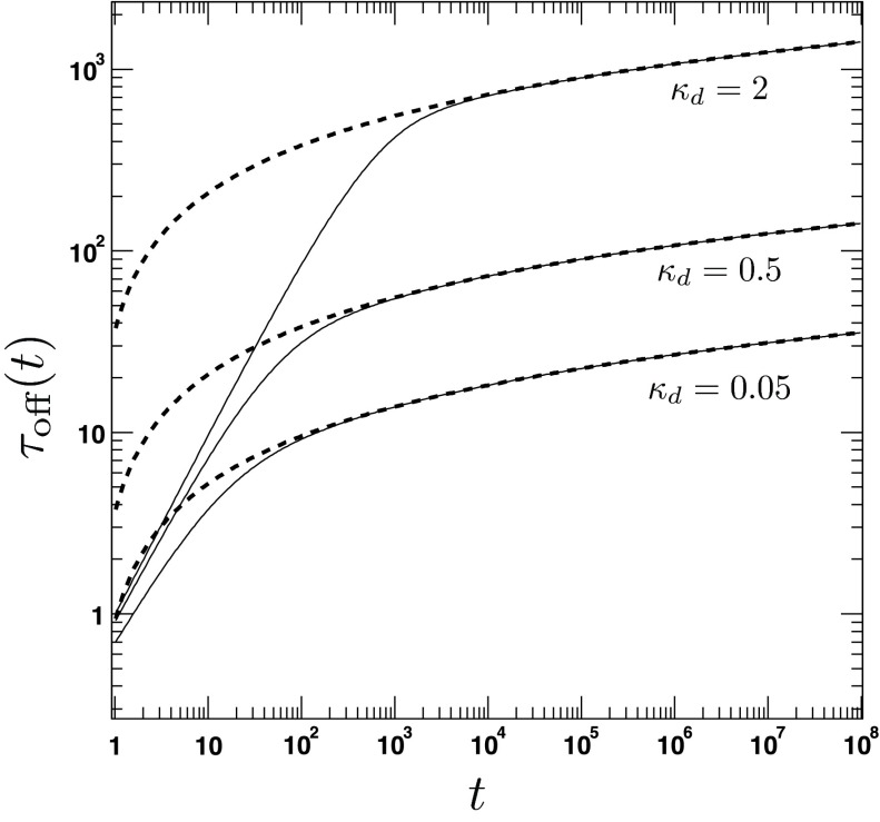
The time dependence of the average lifetime according to the exact and the approximate expression (Eqs. (117) and (124)) is shown in Fig. 8. We find that the obtained expression is similar to the one predicted by CR theories.²² However, one important difference is that the average lifetime depends quadratically on the encounter radius, reflecting the presence of a reaction area πa², while in the CR case this dependence is only implicit and the a² factor can be considered to be absorbed in the intrinsic radiation BC constant κ_a. Note that although both 1/k_irr(t) and τ_off(t) diverge for t → ∞, one has, defining k_off(t) ≡ 1/τ_off(t),

$$\underset{t\to \infty }{\lim }\frac{k_{\text{irr}}\left(t\right)}{k_{\text{off}}\left(t\right)}=\frac{\pi a^2{\kappa }_r}{{\kappa }_d}=K_{\text{eq}},$$ (125)

because the logarithmic divergence cancels out, as one can infer from Eqs. (85) and (124).

FIG. 8.

The average lifetime τ_off(t) of the bound state. The figure shows the time dependence of τ_off(t) for different values of the intrinsic dissociation rate κ_d = 0.05, 0.5, 2. The other parameters are a = 1.5, D = 1, κ_r = 5. The solid lines are obtained from the exact analytical expression for τ_off(t) (Eqs. (117)). The dashed lines refer to the approximate long-time solution (Eq. (124)).

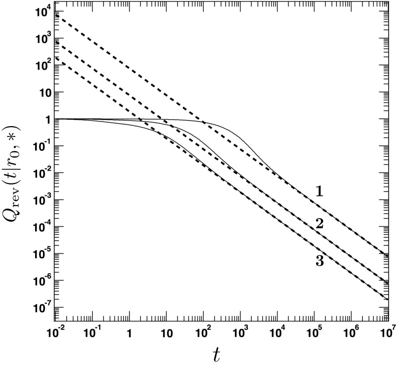
Finally, we turn to the large time approximation of the binding probability of the initially bound state. We employ Eqs. (119) and (121), furthermore we take into account Ch. 13.6, Eq. (8) in Ref. 18

$${\mathbf{L}}^{-1}\left[\ln \left(bs\right)\right]=-\frac{1}{t},$$ (126)

where b > 0 denotes an arbitrary constant, to derive

$$Q_{\text{rev}}\left(t\right|r_0,*)\underset{t\to \infty }{\to }\frac{{\kappa }_r}{{\kappa }_d}\frac{a^2}{4Dt},$$ (127)

see Fig. 9.

FIG. 9.

The binding probability for an initially bound molecule located inside the reaction area at r₀ = 1. The figure shows the time dependence of the binding probability for different values of the intrinsic dissociation constant κ_d = 0.05, 0.5, 2. The other parameters are a = 1.5, D = 0.75, κ_r = 5. The solid lines are obtained from the analytical expression for Q(t|r₀, *).⁴ The dashed lines refer to the long-time approximation (Eq. (127)).

IV. SUMMARY

Prior work on the AR model mainly focused on deriving exact expressions for the GF and survival/binding probabilities of an isolated pair,⁴ see also Refs. ^1–3 for the 3D case. However, a unified and coherent framework, as has been established for CR theories, was still lacking, leaving open the question whether and if yes, how powerful relationships in the context of the CR model, for instance, between the rate coefficient and the single pair survival probability, can be translated to the AR context.

Here, we developed a general framework for the AR model and considered both the irreversible and reversible reaction. Similar to the CR case, we derived relationships between single pair quantities and the reactive flux that is classically identified as the rate coefficient, which plays an essential role in the Smoluchowski theory of homogenous bimolecular reactions. Building on these relationships, we found that the usual definition of the rate coefficient as the reactive flux at the encounter distance is actually deficient for the AR model. By deriving the equation of motion of the many-particle survival probability in the context of pseudo-first-order reactions, we showed that another term, besides the flux, has to be taken into account to describe the reaction rate within the reaction area (Eq. (62)). In this context, we studied how two different initial conditions for the radial distribution function influence the rate coefficient (Figs. 4 and 5) and hence the many-particle survival probability. We provided numerical tests for these findings by performing Brownian Dynamics simulations that showed excellent agreement (Fig. 3). Furthermore, starting from the obtained relationships, we derived short- and long-time approximations of the rate coefficient (Eqs. (77), (79), and (85)) and showed that the short-time behavior is different from its classical counterpart.

For the reversible reaction, we proceeded analogously to the irreversible case and derived several relationships that connect the reversible rate coefficient to single pair quantities. In this way, we showed that the time integral over k_rev(t) gives the equilibrium constant, without the need to use an explicit expression for the rate coefficient (Eqs. (109) and (110)). Also, we derived large-time approximations for the average lifetime and binding probability of the bound state (Eqs. (124) and (127)). We found that these expressions are quite reminiscent to their CR counterparts, but they are explicitly proportional to the reaction area a², while in the CR case this dependence is only implicit and the a² factor can be considered to be absorbed in the intrinsic radiation BC constant κ_a.

We believe that, in addition to its conceptual advances, the theoretical framework presented in this article provides a solid starting point to develop computational models that implement the AR model effectively and accurately, especially for biologically relevant systems.

APPENDIX: EXACT EXPRESSIONS FOR RATE COEFFICIENTS

Exact expressions for the irreversible rate coefficients $k_{\text{rate}}^{\rho =1}\left(t\right)$ and $k_{\text{rate}}^{\rho =1}\left(t\right)$ can easily be obtained from the results that have been obtained for the reversible case.⁴ Using Eqs. (42) and (62) (or, alternatively, (63)) as well as Eq. (99) in Ref. 4 and taking the limit κ_d → 0, we have

$$\begin{array}{ccc}\hfill k_{\text{rate}}^{\rho =1}\left(t\right)& =& \frac{8{\kappa }_r^2}{\pi }[{\int }_{\sqrt{\frac{{\kappa }_r}{D}}}^{\infty }{e}^{-D{x}^{2}t}\frac{{\left(P^{\left(1\right)}(x,a)\right)}^2}{D{x}^2-{\kappa }_r}\frac{dx}{x^3}\hfill \\ & & -{\int }_0^{\sqrt{\frac{{\kappa }_r}{D}}}{e}^{-D{x}^{2}t}\frac{{\left(P^{\left(2\right)}(x,a)\right)}^2}{D{x}^2-{\kappa }_r}\frac{dx}{x^3}],\hfill \end{array}$$ (A1)

where P⁽¹⁾(x, a), P⁽²⁾(x, a) can be obtained from their reversible counterparts, given in Ref. 4, Eqs. (93) and (94), by setting κ_d to zero. The functions P⁽¹⁾(x, a), P⁽²⁾(x, a) are related to the functions T⁽¹⁾(x, r), T⁽²⁾(x, r) that appear in Eq. (99) in Ref. 4 by

$${\int }_0^a{T}^{(1,2)}(x,r)rdr=\frac{a}{x{\xi }_{1,2}}{P}^{(1,2)}(x,a),$$ (A2)

because ${\int }_0^{x}z{J}_0\left(z\right)dz=x{J}_1\left(x\right),{\int }_0^{x}z{I}_0\left(z\right)dz=x{I}_1\left(x\right)$, which follows from Eqs. (9.1.30) and (9.6.28) in Ref. 20. Similarly, using Eq. (66), we obtain

$$\begin{array}{ccc}\hfill k_{\text{rate}}^{\rho =\Theta }\left(t\right)& =& \frac{8{\kappa }_r}{\pi }[{\int }_0^{\sqrt{\frac{{\kappa }_r}{D}}}{e}^{-D{x}^{2}t}{\left(P^{\left(2\right)}(x,a)\right)}^2\frac{dx}{x^3}\hfill \\ & & -{\int }_{\sqrt{\frac{{\kappa }_r}{D}}}^{\infty }{e}^{-D{x}^{2}t}{\left(P^{\left(1\right)}(x,a)\right)}^2\frac{dx}{x^3}],\hfill \end{array}$$ (A3)

where we now employed the relations

$$\frac{\partial }{\partial r}{T}^{(1,2)}(x,r)=-x{\xi }_{1,2}{P}^{(1,2)}(x,r),$$ (A4)

that results from Eqs. (9.1.28) and (9.627) in Ref. 20.

REFERENCES

- 1.Lipková J., Zygalakis K., Chapman S., and Erban R., SIAM J. Appl. Math. 71, 714 (2011). 10.1137/100794213 [DOI] [Google Scholar]
- 2.Khokhlova S. and Agmon N., Bull. Korean Chem. Soc. 33, 1020 (2012). 10.5012/bkcs.2012.33.3.1020 [DOI] [Google Scholar]
- 3.Khokhlova S. and Agmon N., J. Chem. Phys. 137, 184103 (2012). 10.1063/1.4764357 [DOI] [PubMed] [Google Scholar]
- 4.Prüstel T. and Meier-Schellersheim M., J. Chem. Phys. 140, 114106 (2014). 10.1063/1.4868554 [DOI] [PMC free article] [PubMed] [Google Scholar]
- 5.Gösele U., Prog. React. Kinet. 13, 63 (1984). [Google Scholar]
- 6.Rice S., Diffusion Limited Reactions (Elsevier, New York, 1985). [Google Scholar]
- 7.Collins F. and Kimball G., J. Colloid Sci. 4, 425 (1949). 10.1016/0095-8522(49)90023-9 [DOI] [Google Scholar]
- 8.von Smoluchowski M., Z. Phys. Chem. 92, 129 (1917). [Google Scholar]
- 9.Goodrich F., J. Chem. Phys. 22, 588 (1954). 10.1063/1.1740130 [DOI] [Google Scholar]
- 10.Agmon N., J. Chem. Phys. 81, 2811 (1984). 10.1063/1.447954 [DOI] [Google Scholar]
- 11.Kim H. and Shin K., Phys. Rev. Lett. 82, 1578 (1999). 10.1103/PhysRevLett.82.1578 [DOI] [Google Scholar]
- 12.Prüstel T. and Meier-Schellersheim M., J. Chem. Phys. 137, 054104 (2012). 10.1063/1.4737662 [DOI] [PMC free article] [PubMed] [Google Scholar]
- 13.Wilemski G. and Fixman M., J. Chem. Phys. 58, 4009 (1973). 10.1063/1.1679757 [DOI] [Google Scholar]
- 14.Agmon N. and Szabo A., J. Chem. Phys. 92, 5270 (1990). 10.1063/1.458533 [DOI] [Google Scholar]
- 15.Agmon N., Chem. Phys. 370, 232 (2010). 10.1016/j.chemphys.2009.11.004 [DOI] [Google Scholar]
- 16.Naqvi K., Chem. Phys. Lett. 28, 280 (1974). 10.1016/0009-2614(74)80073-4 [DOI] [Google Scholar]
- 17.Szabo A., J. Phys. Chem. 93, 6929 (1989). 10.1021/j100356a011 [DOI] [Google Scholar]
- 18.Carslaw H. and Jaeger J., Conduction of Heat in Solids (Clarendon Press, New York, 1986). [Google Scholar]
- 19.Barzykin A. and Tachiya M., J. Chem. Phys. 99, 9591 (1993). 10.1063/1.465491 [DOI] [Google Scholar]
- 20.Abramowitz M. and Stegun I., Handbook of Mathematical Functions with Formulas, Graphs, and Mathematical Tables (Dover, New York, 1965). [Google Scholar]
- 21.Prüstel T. and Meier-Schellersheim M., e-print arXiv:1112.4010v1 [math-ph].
- 22.Prüstel T. and Meier-Schellersheim M., e-print arXiv:1210.1265v1 [math-ph].