The Effects of Changing Water Content, Relaxation Times, and Tissue Contrast on Tissue Segmentation and Measures of Cortical Anatomy in MR Images

Abstract

Water content is the dominant chemical compound in the brain and it is the primary determinant of tissue contrast in magnetic resonance (MR) images. Water content varies greatly between individuals, and it changes dramatically over time from birth through senescence of the human life span. We hypothesize that the effects that individual- and age-related variations in water content have on contrast of the brain in MR images also has important, systematic effects on in vivo, MRI-based measures of regional brain volumes. We also hypothesize that changes in water content and tissue contrast across time may account for age-related changes in regional volumes, and that differences in water content or tissue contrast across differing neuropsychiatric diagnoses may account for differences in regional volumes across diagnostic groups.

We demonstrate in several complementary ways that subtle variations in water content across age and tissue compartments alter tissue contrast, and that changing tissue contrast in turn alters measures of the thickness and volume of the cortical mantle: (1) We derive analytic relations describing how age-related changes in tissue relaxation times produce age-related changes in tissue gray-scale intensity values and tissue contrast; (2) We vary tissue contrast in computer-generated images to assess its effects on tissue segmentation and volumes of gray matter and white matter; and (3) We use real-world imaging data from adults with either Schizophrenia or Bipolar Disorder and age- and sex-matched healthy adults to assess the ways in which variations in tissue contrast across diagnoses affects group differences in tissue segmentation and associated volumes.

We conclude that in vivo MRI-based morphological measures of the brain, including regional volumes and measures of cortical thickness, are a product of, or at least are confounded by, differences in tissue contrast across individuals, ages, and diagnostic groups, and that differences in tissue contrast in turn likely derive from corresponding differences in water content of the brain across individuals, ages, and diagnostic groups.

1. Introduction

In vivo morphological measures of the brain from anatomical MR images have been used extensively for identifying, localizing, and quantifying both normal brain development and the anatomical disturbances associated with neurological and psychiatric illnesses. Those in vivo, MRI-based measures are assumed to relate directly and invariantly to ex vivo histological measures of the same tissue. The relation between in vivo and ex vivo measures has been largely untested, however, in part because in vivo measures are difficult, if not impossible, to relate directly to the ex vivo ones, owing partly to fixation artifacts that affect postmortem tissue, and partly to the fact that some of the most important determinants of image characteristics, particularly tissue contrast, may affect in vivo MR measures but have no effect on the ex vivo histological measures. Systematic and regionally specific variations of these determinants across the brain either with age in healthy individuals or between healthy and diseased populations may cause variations in in vivo morphological measures that cannot be related to the ex vivo histological ones. Thus, careful assessment of and controlling for the effects of variations in these determinants on in vivo measures is important for understanding better the biological processes associated with both normal brain maturation and brain pathology.

Gray scale intensity and tissue contrast at each voxel of an MR image are determined solely by the longitudinal (T1) relaxation time, transverse (T2) relaxation time, and proton density of the tissue represented in that voxel. Relaxation times, in turn, depend upon the cellular and molecular characteristics of that tissue, including the density of cells and neuropil (i.e., dendrites, axonal terminals, and unmyelinated axons), iron concentration¹, the relative proportion of various macromolecules^{2, 3}, the complexity of cellular appendages, and intra- and extra-cellular water content. Because gray and white matter have distinctively differing cellular properties and can usually be differentiated unambiguously in histological preparations, identification of voxels as gray matter (GM) or white matter (WM) in MR images and measurement of morphological properties also have been assumed to be clear and unambiguous. In vivo measures of either overall or regional GM and WM volumes have been presumed valid and independent of subtle variations in the underlying cellular and molecular properties of the tissues being measured, just as ex vivo histological measures^4-7 are assumed to be independent of those same cellular and molecular properties.

We hypothesize that morphological measures^8-13 of regional shapes and volumes in MR images depend upon the contrast between GM, WM, and CSF tissues, and because contrast depends on relaxation times and relaxation times in turn depend upon the molecular and cellular characteristics of the tissue being imaged, in vivo measures of regional shapes and volumes, unlike ex vivo histological measures, will also ultimately depend upon the water content of the tissue, which can vary considerably across people and across ages. In other words, MRI-based measures of shape and volume are not as fixed and invariant as they generally are assumed to be, as they are heavily influenced by local variations in water content of the tissue.

The water content of brain tissue varies regionally,¹⁴ and within a given brain region it varies nonlinearly with age³. In healthy adults, water content in GM decreases by 0.034% per year, whereas in WM it increases with age.^15-18 The change in water content is even more dramatic within the first week of life, decreasing from 95% of tissue volume in 34-week old infants to 82% in 54-weeks old infants¹⁶, and it continues to decrease further thereafter.¹⁵ These rapid, age-related decreases in water content in the neonate produces rapid changes in the T1- and T2-relaxation times of brain tissues and subsequent dramatic changes in tissue contrast¹⁹. For nonadipose tissue, the time for T1 relaxation in a 1.5 Tesla MRI scanner has been modeled as T1 = 7.94w–5.16 ms, where w is water content of the tissue.²⁰ Moreover, relaxation times and tissue contrast change in a regionally specific manner across the brain because the rate of change in water content differs regionally across the brain. Thus, because tissue intensity is determined primarily by water content, variations of which do not generally affect ex vivo histological measures, we assessed the effects of previously reported variations in water content on in vivo measures from MR images of the brain.

We hypothesize that computer algorithms for tissue segmentation yield thinner measures of the cerebral cortex in images that have lower tissue contrast. We provide support for this hypothesis in several ways: (1) We derive three analytic relations between (a) the change in tissue intensity and the change in relaxation times, (b) the change in relaxation times and the change in tissue contrast, and (c) the change in tissue contrast and the change in tissue definition. These analytic relations allow us to conclude whether we should expect a change in tissue contrast and cortical thickness with a change in water content and relaxation times. (2) We use computer-generated, T1-weighted images simulated from brain-wide maps of previously reported relaxation times at various ages. Because the ground truth definitions of GM and WM are known in these simulated images, their values allow us to establish precisely the effects that regionally specific, spatially varying age-related changes in tissue contrast have on tissue definition. (3) We also use T1-weighted images of adults who are healthy or who have either Schizophrenia (SZ) or Bipolar Disorder (BD) to assess whether tissue contrast can differ across diagnostic groups and whether those differences in tissue contrast can substantially affect in vivo MR measures of brain morphology. Demonstrating that these changes in water content, relaxation times, and tissue contrast have substantial effects on MRI-based measures of brain structure has profound implications for the field of brain imaging and fundamentally calls into question the validity of what we thought we had learned until now about brain maturation and the pathophysiologies of neuropsychiatric illnesses.

2. Methods

2.1 Overview

We assessed the effects of change in tissue intensity and contrast on the segmentation and regional definition of brain tissue by deriving the analytic relations between these values and by demonstrating their influences on anatomical measures from computer-generated and real-world MR images of the brain.

1. We evaluated the effects of variations in image contrast on tissue segmentation using (a) three sets of computed-generated images and (b) a large set of images from healthy adults and adults with psychiatric illnesses.

   1. Each of the computer-generated datasets consisted of T1-weighted images representing a baseline image of the brain and additional T1-weighted images representing the same brain but with tissue contrast and relaxation times modeled as changes over 10-year increments based on previously published normative values for relaxation times at varying ages. We segmented brain tissue in the baseline image as either GM or WM by applying (i) a histogram-based method that modeled image intensities using a Gaussian mixture model and applied Expectation maximization algorithm to label voxels as either GM or WM, and (ii) a Markov Random Field (MRF)-based method that modeled voxel intensities as a MRF to enfore a regional homogeneity contrast and generated maps of tissue that were spatially contiguous. The cortex identified in the baseline image was considered the gold-standard definition with which was compared the cortical definition in simulated brains at subsequent ages, thereby allowing us to compute the change in thickness with age that is a function only of age-related changes in relaxation times and proton density and their effects on tissue contrast.
   2. We also used imaging data from 79 adults with Schizophrenia (SZ) and their age-matched 66 healthy adults, and 37 adults with Bipolar Disorder (BD) and their age-matched 58 healthy adults to assess the effects of real illness-related variation in tissue contrast on measures of cortical thickness across diagnoses. We expected that presumed age-related declines in water content would reduce tissue contrast and thereby would reduce volumes and thickness of cortical gray matter, and we likewise anticipated that patient populations with lower tissue contrast would also have reductions in measured volumes and thicknesses of their cortical gray matter. We also expected that the regional pattern of differences in cortical thickness between healthy and patient populations would match the spatial pattern of changes in cortical thickness with age that we detected in our computer-generated images, suggesting that regional variations in group differences across patient populations may be attributable more to local variations in water content than to real differences in morphological characteristics of the underlying tissue.

2. Finally, we derived analytic relations between a given change in relaxation times and the corresponding change in tissue intensity and contrast of the image. In addition, we showed analytically that the change in tissue contrast would cause misclassifications of both GM and WM, and in equal proportions.

2.2 Tissue Segmentation

We briefly describe the two automated methods that we used to segment brain tissue at each voxel of the image as being either GM or WM. These two methods for tissue segmentation either are implemented directly within or they form the bases for more advanced methods in the most commonly used toolboxes for image processing, including Bioimage Suite²¹, FreeSurfer²², SPM5²³, and FSL-FAST⁹.

1. Histogram-Based Segmentation This method modeled the distributions of GM and WM voxel intensities as Gaussian distributions having means μ₁ and μ₂ and variances σ₁ and σ₂. We estimated the empirical distributions of each class of brain tissue by forming the histogram for the entire image and then using a K-means clustering algorithm to estimate optimal values for the means and variances of each tissue type.^{24, 25} The clustering algorithm initialized the means μ₁ and μ₂ and variances σ₁ and σ₂ from the histogram of image intensities for the entire brain. Using these initialized values, the algorithm iterated the two operations until the estimated means and variances converged to a specific value. The first operation of the algorithm used the current estimates of the means and variances to compute the likelihood that each voxel belonged to either GM or WM, and then assigned each voxel to the class with the higher likelihood. In the second operation, the means and variances for the two classes were updated using the intensities of the voxels assigned to that class. The algorithm converged to a particular assignment of voxels to GM and WM if the changes in the means and variances from one iteration to another were smaller than a specified threshold.

2. MRF-Based Segmentation In the presence of noise, the histogram-based method generates tissue definitions that are not spatially contiguous. To reduce noise in the segmented images and to yield tissue definitions that are spatially homogeneous, an MRF-based segmentation constrained the tissue classification of each voxel by the tissue type of its neighboring voxels, thereby generating spatially contiguous classifications. The constraint requiring a homogeneous neighborhood was imposed using a Gibbs distribution as a prior on the expected segmentations, and the voxel intensities were incorporated using a likelihood term of the observed intensity at that voxel for its current tissue type.²⁶ The optimal tissue type for each voxel was then estimated using an expectation maximization algorithm.²⁷ Although prior validation studies have shown these methods to be robust in the presence of noise²⁸, those studies have not evaluated the effects of changing tissue contrast on the estimated segmentation of brain tissue.

2.3 Image Preprocessing

We isolated brain from nonbrain tissue in our real human images. First, we corrected intensity inhomogeneities using an automated algorithm²⁹ that models those inhomogeneities as a multiplicative field. Second, brains were reoriented into a standard orientation in which the anterior and posterior commissures were positioned in the same transverse slice and in which landmarks within the interhemispheric fissure were placed in the same sagittal plane. Finally, brain was isolated from nonbrain tissue using a semi-automated technique that first used an automated tool³⁰ to define the surface of the brain, which was then edited manually in the three orthogonal views to remove connecting dura.

2.4 Computer-Generated Brains

2.4.0. Overview

We created three sets of computer-generated brains that modeled empirically determined, age-related changes in tissue intensity and contrast: (1) In the first set (described in detail in section 2.4.1 below), we progressively reduced tissue contrast by increasing only gray-scale intensity values of GM voxels proportionately with increasing age based on empirically determined, age-related changes in GM intensities, while keeping the intensities of WM voxels constant. (2) In the second set (described in section 2.4.2), brains were generated using simulated maps of T1 and T2 relaxation times based on published values for GM and WM and then varying those values with age according to previously reported cross-sectional studies¹⁴. (3) In the third set (described in section 2.4.3), brains were generated using real maps of T1 and T2 relaxation times obtained from a single healthy adult and then varying those values progressively with age. We generated the images in the second and third sets by varying the T1 and T2 relaxation times at rates published in the literature. The relevant sections below provide the rationales for constructing and assessing contrast effects in each of these synthetic datasets.

In all three of these datasets, in both the simulated and real-world maps of relaxation times, we assumed that a single T1 and single T2 relaxation time measured the average relaxation times within each voxel. The T1-weighted images at differing ages in the second and third sets of computer-generated brains were reconstructed from maps of relaxation times. For the images in the second set, the T1-weighted image used to construct synthetic maps of relaxation times was acquired on a 1.5T MRI scanner with spatial resolution of 1.2mm × 1.17mm × 1.17mm. On the other hand, for images in the third set, the images used to construct the real maps of relaxation times were acquired on a 3T MRI scanner at an isotropic spatial resolution of 1.0 mm³. The voxel size of a brain at 3T was 39% smaller than the voxel size of a brain at 1.5T. Because the brains acquired using the two scanners had differing spatial resolutions, relaxation times, intensity inhomogeneities, and signal-to-noise and contrast-to-noise ratios, we always treated the data from the two scanners independently and never combined in any of our experiments. In each of these three simulated datasets, the brain at the youngest age was termed the baseline image and the segmented cortices defined in brains at differing ages were compared with that baseline image to assess the effects of changing tissue intensity and contrast on the definition of cortical GM.

2.4.1 Computer-Generated Images with Age-Related Increases in GM Intensities

For the first set of computer-generated images, we selected one brain as a baseline image and then generated brains at increasing ages by progressively increasing GM intensities. Brain tissues in the baseline image were segmented as GM or WM using MRF. The GM intensities were progressively increased to generate brains with progressively decreasing tissue contrast simulating the brains of persons between 20 and 65 years of age. The rate of increase in GM intensities was estimated empirically from the T1-weighted images of 43 healthy participants, ages 10 to 57 years old.

These T1-weighted images were acquired using a 1.5T Siemens MRI scanner and were preprocessed and segmented using the same semi-automated procedures described for preprocessing datasets in the present study. For segmenting the brain as GM or WM, we sampled pure GM and WM in four different regions of the brain using a 4-by-4 window, a sampling window small enough to provide samples of pure GM and WM intensities and avoid partial volume effects but sufficiently large to provide stable representations of tissue intensity in each region. The GM and WM intensities were then averaged across sampling windows.

We computed tissue contrast as the ratio of the difference in the average WM (AveWM) and average GM (AveGM) values divided by the average GM intensity: Percent Contrast = 100·(AveWM − AveGM)/AveGM. In our empirical dataset of healthy participants, tissue percent contrast decreased linearly by 0.124 units per year (Fig.1). Therefore, contrast C_x at age x years as a function of contrast C₂₀ at age 20 years was calculated as C_x = C₂₀ – 0.00124 (x − 20). Modeling age-related reductions in tissue contrast by keeping WM intensities constant and increasing only GM intensities, the average GM intensity ${\overline{\mathit{\text{GM}}}}_x$ at age x years was calculated as ${\overline{\mathit{\text{GM}}}}_x=\left[\frac{{\overline{\mathit{\text{WM}}}}_{20}}{1+C_x}\right]$ Where ${\overline{\mathit{\text{WM}}}}_{20}$ was the average WM intensity at age 20 years. The GM intensity GM_x of each voxel in the computer-generated brain at age x years was then computed by adding the difference in the average intensities ${\overline{\mathit{\text{GM}}}}_x$ and ${\overline{\mathit{\text{GM}}}}_{20}$ of gray matter to the intensity GM₂₀ at age 20 years, i.e. ${\mathit{\text{GM}}}_x={\mathit{\text{GM}}}_{20}+({\overline{\mathit{\text{GM}}}}_x-{\overline{\mathit{\text{GM}}}}_{20})$.

Fig.1. Changes in Tissue Contrast with Age and Changes in Cortical Thickness with Tissue Contrast.

In our cohort of 43 healthy participants (age 10 years to 57 years), tissue percent contrast decreased 0.124 per year (p < 0.02) and cortical thickness increased 0.0462mm per year (p = 0.002) with increasing contrast. The percent tissue contrast was computed as (AveWM-AveGM)/AveGM * 100, where AveWM is the average intensity in white matter (WM) and AveGM is the average intensity in gray matter (GM). Average cortical thickness was computed by averaging thickness at each voxel across the entire surface of the brain. These plots showed that the tissue contrast decreased with age and that automated methods for tissue segmentation defined thicker cortex in MR images with higher tissue contrast.

2.4.2 Synthetic Maps of Age-Related Changes in T1 and T2 Relaxation Times

The second set of computer-generated images was constructed by first creating synthetic maps of T1 and T2 relaxation times for the baseline image using previously reported relaxation times measured with a 1.5T scanner¹⁴. Then the maps of relaxation times were modified using previously reported age-related changes in both relaxation times and water content^{14, 31}. Finally, the age-specific synthetic maps of relaxation times were used to reconstruct T1-weighted images at each corresponding age. The maps of relaxation times should have modeled age-related variation in tissue intensities more accurately than the first set of synthetic images (in 2.4.1) because they modeled age-related changes in both the relaxation times and water content of GM and WM tissues, and they varied relaxation times continuously and smoothly across voxels from the GM/WM boundary to account for partial volume effects and similar water content. Because relaxation times decrease in GM with age, we expected that tissue contrast in the images reconstructed from maps of relaxation times would decrease progressively with increasing age.

Synthetic Maps at Baseline To generate maps of T1- and T2-relaxation times for the baseline image, we first used MRF to segment the T1-weighted image as GM or WM. We then removed GM from the image and used a 3D morphological operator³² to distance-transform the image to generate at each voxel within GM and WM the distance of that voxel from the GM/WM boundary. We then used the distance of the voxel from the GM/WM boundary to specify the T1 and T2 relaxation times for each voxel. Relaxation times for both GM and WM are Gaussian distributed¹⁴ and we expected T1 and T2 relaxation times of voxels within pure GM and WM to equal the previously reported modal values of 1250 ms and 94 ms for GM and 560 ms and 87 ms for WM, respectively, in a 1.5T scanner for a 23-year old healthy adult¹⁴. Furthermore, we modeled equal relaxation times for voxels along the GM/WM boundary because of the partial volume effects and similar water content in voxels at those locations. Therefore, we set relaxation times for these voxels to the average of their modal values (i.e., 900 ms for T1 and 90 ms for T2 relaxation times). Assuming that voxels located at a distance of two or more voxels from a GM/WM interface represent true GM and WM, we set their relaxation times to the modal reference values of the healthy adult¹⁴. Finally, we ensured that relaxation times would vary smoothly across the maps by setting the T1 and T2 times of voxels immediately adjacent to the GM/WM interface to 1075 ms and 92 ms in GM, and 730 ms and 88.5 ms in WM. In these synthetic maps, however, the relaxation times changed uniformly as a distance from the GM/WM boundary, and this change in relaxation times was identical from one region of the brain to another. Using maps of relaxation times that vary smoothly across the GM/WM boundary would generate images with smaller variation in tissue contrast with age and therefore should yield a conservative estimate of the effect of varying water content on tissue definition.

Synthetic Maps at Varying Ages Maps of relaxation times at differing ages were generated using previously reported values^{14, 31}. T1 declines linearly in GM by 2.3 ms each year¹⁴ and increases in WM by 1.34 ms each year³¹, whereas T2 increases 0.05 ms each year in both GM and WM³¹. To minimize the influence of tissue segmentation on age-related changes in relaxation times, we changed relaxation times at a rate based on relaxation times in the baseline image. We therefore changed the relaxation times of the voxels along the GM/WM boundary at a rate that was the average of the rates for pure GM and WM – i.e., reducing T1 by 0.48 ms each year for voxels in both GM and WM along the GM/WM boundary. For voxels immediately adjacent to the interface, we reduced T1 times for GM by 1.39 ms each year and increased them for WM voxels by 0.43 ms each year to account for the smoothly varying values caused by partial volume effects and similar water content in those voxels. Therefore, smoothly varying relaxation times across the image would yield smaller changes in those values with age, thereby producing smaller age-related changes in tissue contrast than voxels in a real-world dataset. Therefore, our simulated dataset yielded a more conservative estimate of a change in tissue contrast, and therefore it also yielded a more conservative estimate of change in cortical thickness with age. Finally, the water content of brain tissue, and therefore proton density and signal strength, decreases in GM from 81% at age 20 years to 79% at age 75 years, and it increases in WM from 69% at age 20 years to about 71% at age 75 years¹⁵. Consistent with the increase in water content of WM, in the simulated dataset we increased the proton density and signal intensity across WM with age, thereby reducing the rate of decrease in tissue contrast with age.

Reconstructing T1-weighted Images From the synthetic maps of T1- and T2-relaxation times, we reconstructed T1-weighted brain images at various ages using the well known relation between MRI signal strength and T1 and T2 relaxation times. MRI signal S_v from a voxel v is modeled as S_v = S_v,0 · PD_v · 1 − exp −TR/T1_v ·exp(−TE/T2_v) where S_v,0 is the maximum MRI signal strength and PD_v is the proton density of the voxel, and where TR is the repetition time and TE is the echo time of the pulse sequence used to acquire the T1-weighted image. The detected MR signal S_v is processed in the scanner console to generate a T1-weighted image with intensity I_v at voxel v. We will assumed that I_v is directly proportional to S_v-- i.e., I_v=C_v · S_v = K_v · [1−exp −TR/T1_v] ·exp −TE/T2_v , where K_v is a constant for an MRI scanner that varies from one scanner to another. Using the baseline maps for T1 and T2 relaxation times, and using TR = 600 ms and TE = 3.4ms for a typical T1-weighted image acquired on a 1.5T scanner, we computed the map of K_v for all voxels across the brain. We then used the map K_v and the synthetic maps of relaxation times at various ages to reconstruct the T1-weighted images at each of those ages. Finally, because the water content of tissue changes with age, which in turn affects signal intensity by changes in proton density, we multiplied the intensities of GM voxels by − 2· x – 20 / 55 + 81 /81 and those of WM voxels by 2· x − 20 / 55 + 70 / 70, where x is the age of the reconstructed brain, and 81% GM and 70% WM water content at age 20 years. Each of these age-specific, computer-generated T1-weighted images was segmented using both the histogram- and MRF-based methods. The GM thickness at each age were compared to the GM thickness of the baseline image to assess the age-related changes in cortical thickness attributable to the tissue's changing water content.

These synthetic maps of relaxation times more accurately modeled age-related variation in tissue intensities than did maps in the first synthetic dataset because they modeled age-related changes in both relaxation times and water content of GM and WM tissues, and because they varied relaxation times smoothly across voxels at the GM/WM boundary to account for both their partial volume effects and similar water contents. However, relaxation times and age-related changes in those values were distributed uniformly across the entire brain, thereby yielding a uniform change in tissue intensity and contrast throughout the brain. The third synthetic dataset was designed to address this limitation of uniformity in intensity and contrast across the brain.

2.4.3 Synthetic Maps of Age-Related Changes in T1 and T2 Relaxation Times Constructed from Baseline Maps of Relaxation Times in a Healthy Participant

Unlike the uniform distribution of relaxation times as modeled for brains in our second synthetic dataset, relaxation times and water content in real-world data vary from one region to another. To generate images with realistic regional variations in tissue intensities, we acquired baseline maps of T1 and T2 relaxation times and a baseline T1-weighted image in a healthy adult. We then generated synthetic T1-weighted images at various ages by varying relaxation times using previously published, age-specific values for relaxation times, just as we did for the second set of synthetic images. Because the variation in relaxation times across the brain depended upon variations in relaxation times and water content across the brain at baseline, the synthetic images representing age-related changes in relaxation times, water content, and contrast that depended on them also varied regionally across the brain.

T1-weighted Image The imaging data for the healthy adult were acquired using a 3 Tesla, whole body, GE Signa HDx scanner (GE Medical Systems, Milwaukee, WI), ASSET (Array Spatial Sensitivity Encoding Technique)-based parallel imaging capability (acceleration factor R=2), and an 8-channel head coil (Invivo Corporation, Orlando, FL). The anatomical T1-weighted image was acquired using a three-dimensional, fast spoiled gradient-echo (FSPGR) pulse sequence in the sagittal orientation with inversion time (TI) = 500 ms, echo time (TE) = 2.38 ms, slice thickness = 1.0 mm, flip angle = 11°, Field of View (FOV) = 25 cm, and acquisition matrix = 256 × 256.

Map of T1 Relaxation Times To construct the map of T1 relaxation times, we acquired six brain images in the transverse orientation using an inversion recovery fast spin echo (IR-FSE) pulse sequence with an adiabatic 180° inversion pulse and inversion times (TI) of 60ms, 200ms, 400ms, 700ms, 1300ms, and 2000ms. The other parameters of the pulse sequence, which was held constant for these six brain images, were TE=8.532ms, TR=8000ms, flip angle = 90°, and slice thickness = 3mm, providing an in-plane resolution of 0.9766mm × 0.9766mm. The MRI signal in the IR-FSE sequence was modeled as S = S₀ (1 − 2e^−TI/T₁ + e^{−(TR−TE_last)/T₁})e^{−TE_eff/T₂}, with TE_last = ETL × esp where ETL is the echo train length and esp is the echo spacing between consecutive echoes.³³ We then estimated the optimal value of T1 relaxation for tissue in each voxel by applying a nonlinear, least squares fitting in MATLAB (The MathWorks Inc., Natick, MA).

Map of T2 Relaxation Times We constructed the map of T2 relaxation times from seven brain images acquired using a fast spin echo (FSE) pulse sequence with echo times (TE) 8.532ms, 25ms, 50ms, 75ms, 100ms, 125ms, 150ms, and 175ms. The other pulse sequence parameters were kept constant across the seven images and included TR=3500ms, flip angle = 90°, and slice thickness = 3mm, providing an in-plane resolution 0.9766mm × 0.9766mm. The transverse relaxation time (T2-relaxation) was estimated by modeling the observed MRI signal as³⁴

$$S=S_0(1-2e^{-(\mathit{\text{TR}}-\mathit{\text{TE}}/2)/T_1}+e^{-\mathit{\text{TR}}/T_1})e^{-\mathit{\text{TE}}/T_2}\approx S_0(1-e^{-\mathit{\text{TR}}/T_1})e^{-\mathit{\text{TE}}/T_2}=S_0^{\ast }{e}^{-\mathit{\text{TE}}/T_2}$$

where the approximation holds for TR ≫ TE. We therefore fitted a monoexponential model to the data acquired for various TE's using MATLAB (The MathWorks Inc., Natick, MA) to estimate the optimal value of T2 at each voxel. We used the FSE pulse sequence to acquire the map of T2 relaxation times because we have previously shown³⁵ that both FSE and SE based sequences generate high quality images for computing T2 relaxation times. In fact, several other published studies^36-38 have used FSE for measuring T2 relaxation times. Although relaxation times computed using the two pulse sequences may differ, those differences are small³⁵ (<3%), less than ±3ms in both GM and WM. These differences are smaller than the variance of relaxation times within tissue caused by noise and the differing tissue compositions across the brain. For example, in the adult brain, T2 relaxation times were 93±12.9 ms in gray matter (GM) and 85±10.37 ms in white matter (WM), with a 3-4 times larger variance in relaxation times than the possible variance differences produced by the two different pulse sequences. Furthermore, the small bias in relaxation times across the two pulse sequences will obtain across all ages of our participants and therefore cannot account for the changes in tissue contrast with age that we have detected.

Coregistering Images We coregistered the maps of T1 and T2 relaxation times to the T1-weighted image using a similarity transformation (three translations and three rotations) such that the mutual information³⁹ between the coregistered images was maximized. We then used MRF to segment the baseline T1-weighted image and computed the average values of T1 and T2 times in GM and WM. Let T1^GM and T2^GM be the average T1 and T2 relaxation times in GM, and T1^WM and T2^WM be the average T1 and T2 relaxation times in WM. We then generated T1-weighted images for various ages by first varying the relaxation times using previously published values and then computing MR signal for each voxel. In a 3T MRI scanner, T1 relaxation times in GM decline 1.7 ms each year¹⁴ and in WM they increase 1.2 ms each year³¹. At each voxel we linearly varied the relaxation times $T{1}_x^v$ and $T{2}_x^v$ at age x based on its relaxation times $T{1}_b^v$ and $T{2}_b^v$ at baseline:

$$T{1}_x^v=x-20\cdot [-2.9\cdot (\frac{T{1}_b^v-T{1}^{\mathit{\text{WM}}}}{T{1}^{\mathit{\text{GM}}}-T{1}^{\mathit{\text{WM}}}})+1.2]+T{1}_b^v$$

Therefore, T1 relaxation times at voxels having a relaxation time of T1^GM at baseline will decrease 1.7 ms each year, and those with a relaxation time of T1^WM at baseline will increase 1.2 ms each year. Voxels with intermediate T1 relaxation times at baseline will have intermediate rates of age-related change. Therefore, because relaxation times vary smoothly across the baseline image, the rates of age-related change in relaxation times also will vary smoothly across the brain. This smooth variation in rates yields smaller changes in tissue intensities and contrast, and therefore the reconstructed images yield smaller age-related decreases in tissue contrast, than do images in real-world datasets. We assumed that the water content, and therefore proton density, changed by the same amounts as those in the second synthetic dataset.

The data in each of the three sets of computer-generated images were registered to the same brain to ensure that the age-related changes in cortical thickness would be attributable to the effects of changing water content, relaxation times, and tissue contrast on tissue segmentation and not to any confounding effects of brain morphology. We expected that tissue contrast would decrease with age, that automated tools for tissue segmentation would yield a thinner cortex in images with lower tissue contrast, and that therefore progressively older participants would have progressively thinner cortices solely because of declining water content and declining tissue contrast.

2.5 Differences in Tissue Contrast Between Healthy Individuals and Individuals with Psychiatric Illnesses

We expected that the automated tools applied to our computer-generated images would define thinner cortices in images with lower tissue contrast. Therefore, we also expected that if tissue contrast in real-world images of healthy participants differed from those of participants with psychiatric illnesses, then the cortex would be thinner in images of participants with lower tissue contrast. In addition, we expected that the spatial pattern of difference in cortical thickness between healthy and affected individuals would match the spatial pattern of decreasing cortical thickness that we detected in association with declining tissue contrast in the third set of computer-generated images (in section 2.4.3). We therefore compared tissue contrast and cortical thickness in two sets of participants for whom we had acquired T1-weighted brain images.

Sample 1 consisted of 74 adults with Schizophrenia (SZ; 49 males, age 42.00±8.5 years) and 46 healthy adults (HA; 23 males, age 38.7±10.1 years). Adults with SZ were identified from general outpatient clinics and met DSM-IV criteria for Schizophrenia. All participants were on their medications for at least thirty days and had not abused substances for at least sixty days prior to the acquisition of MRI data. Diagnostic assessments were supplemented using the Positive and Negative Symptom Scale for Schizophrenia.^{40, 41}

Sample 2 consisted of 38 adolescents and adults with Bipolar Disorder I (BD; 17 males, age 32.2±13.8 years) and 58 HA (29 males, age 27.7±14.3 years). BD participants were ascertained by a board-certified adult psychiatrist who administered the Structured Clinical Interview for DSM-IV Axis I & II Disorders, Version 2.0⁴² and the participants younger than 18 years were ascertained by a child psychiatrist and a psychologist expert in childhood mood disorders who administered the Schedule for Affective Disorders and Schizophrenia for School-Age Children–Present and Lifetime Version.⁴³

For healthy adults, the exclusion criteria included a lifetime or a current DSM-IV Axis 1 or 2 disorder, and IQ<80. Final DSM-IV diagnoses for all participants were established using a procedure for consensus diagnosis using all available clinical and research materials.^{44, 45}

MR images for these two samples were acquired on a 1.5 Tesla GE scanner using a sagittal spoiled gradient recall sequence (TR=24msec, TE=5msec, 45° flip, frequency encoding S/I, no wrap, 256×192 matrix, FOV=30 cm, 2 excitations, slice thickness=1.2 mm, 124 contiguous slices). The definition of GM and WM allowed us to compute tissue contrast in the brains of all participants. We plotted contrast versus age of the participants in each group to assess change in tissue contrast with age.

We normalized the brains of all participants to a template brain, thereby allowing us to compute and compare statistically the average cortical thickness at each voxel on the surface of the brain for each group of participants. We plotted the correlation of cortical thickness with age at each point of the cerebral surface and compared those correlations across diagnostic groups in each of our two samples of participants. The brain of a healthy participant was selected as a template to which the brains of all other participants were coregistered. Coregistration was performed using first a similarity transformation (3 translations, 3 rotations, and global scaling) that maximized mutual information³⁹ between the brains and then subsequently a high-dimensional, nonlinear warping algorithm⁴⁶ that matched each brain to the exact shape and size of the template. The nonlinear warping therefore established point-by-point correspondences across the surface of each brain to the template surface, allowing us to map cortical thickness for each participant onto the template surface.

We computed cortical thickness within template space as the shortest distance from the pial surface to the surface of white matter using a 3-dimensional morphological operator that distance-transformed the surface of white matter to the surface of the same brain.^{47, 48} At each point on the surface of the template brain, we statistically compared cortical thickness across diagnostic groups and color-encoded the P-value of that statistical difference to generate maps of P-values across the surface of the template brain.

As before, we expected that reduced tissue contrast would yield a thinner cortex. Therefore, diagnostic groups with reduced tissue contrast in their images should have thinner cortices than groups with greater tissue contrast in their images. In addition, we expected that the pattern of reduction in cortical thickness associated with reduced contrast would match the pattern of age-related decline in cortical thickness that is attributable solely to the age-related decline in tissue contrast.

2.6 How Changes in T1 Relaxation Times Produce Changes in MRI Signal Intensity

We expected that changing relaxation times that reduce tissue contrast in computer-generated images would yield thinner cortices defined with automated tools for segmentation. In addition to the empirical evidence that tissue intensities and contrast decrease with age, we derived the relation between changes in relaxation times, changes in tissue intensities, and changes in tissue contrast. First, we derived the relation between changes in T1 relaxation times and proton density on the one hand with changes in tissue intensities on the other. We then used this relation to show how tissue contrast varies with changes in relaxation times and proton density.

As shown in Appendix A, the fractional change in brain tissue signal relates linearly with the change in T1 relaxation times as

$${\left(\frac{{\overline{S}}_v-S_v}{S_v}\right)}_{\mathit{\text{GM}}}\approx \left(\frac{\Delta {\mathit{\text{PD}}}^G}{{\mathit{\text{PD}}}^G}\right)-\frac{\Delta T{1}^{\mathit{\text{GM}}}}{4\cdot \mathit{\text{TR}}\cdot exp\left(0.5\right)-1}=\left(\frac{\Delta {\mathit{\text{PD}}}^G}{{\mathit{\text{PD}}}^G}\right)-6.25\cdot {10}^{-4}\cdot \Delta T{1}^{\mathit{\text{GM}}},$$

and

$${\left(\frac{{\overline{S}}_v-S_v}{S_v}\right)}_{\mathit{\text{WM}}}\approx \left(\frac{\Delta {\mathit{\text{PD}}}^{\mathit{\text{WM}}}}{{\mathit{\text{PD}}}^{\mathit{\text{WM}}}}\right)-\frac{\Delta T{1}^{\mathit{\text{WM}}}}{\mathit{\text{TR}}\cdot (e-1)}=\left(\frac{\Delta {\mathit{\text{PD}}}^{\mathit{\text{WM}}}}{{\mathit{\text{PD}}}^{\mathit{\text{WM}}}}\right)-9.96\cdot {10}^{-4}\cdot \Delta T{1}^{\mathit{\text{WM}}}$$

Where S_v is the MRI signal at voxel v , TR is the repetition time, PD is proton density, and T1 is the T1 relaxation time. These relations show that the intensities of GM voxels change more slowly than those of WM voxels, and that the change is linear, with changing T1 relaxation times. Furthermore, because T1 relaxation decreases in GM and increases in WM with age, these relations suggest that voxel intensities increase in GM and decrease in WM, thereby reduced tissue contrast with advancing age. Moreover, although the fractional change in tissue intensities relates linearly to a change in relaxation times, tissue intensities may change nonlinearly with age if relaxation times change nonlinearly with age.

2.7 How Changes in T1 Relaxation Times Change Tissue Contrast

Using the above relation between tissue intensity and relaxation times, in Appendix B we showed that changes in tissue contrast relate to changes in relaxation times, as follows:

$$[\frac{({\overline{S}}^W-{\overline{S}}^G)}{{\overline{S}}^G}-\frac{(S^W-S^G)}{S^G}]=(1+\frac{(S^W-S^G)}{S^G})[-\frac{\Delta {\mathit{\text{PD}}}^G}{{\mathit{\text{PD}}}^G}+6.25\cdot {10}^{-4}\cdot \Delta T{1}^G]+[1.72\cdot \frac{\Delta {\mathit{\text{PD}}}^W}{{\mathit{\text{PD}}}^G}-17.11\cdot {10}^{-4}\cdot \frac{{\mathit{\text{PD}}}^W}{{\mathit{\text{PD}}}^G}\Delta T{1}^W]=(1+\frac{(S^W-S^G)}{S^G})[-\frac{\Delta {\mathit{\text{PD}}}^G}{{\mathit{\text{PD}}}^G}+6.25\cdot {10}^{-4}\cdot \Delta T{1}^G]+[1.51\cdot \frac{\Delta {\mathit{\text{PD}}}^W}{{\mathit{\text{PD}}}^W}-15.05\cdot {10}^{-4}\cdot \Delta T{1}^W]$$

Because with increasing age ΔT1^G < 0 and ΔT1^W > 0, contrast decreases linearly with age. In addition, brain regions with greater baseline tissue contrast will suffer a larger decline in contrast for the same change in relaxation times with age than will regions where baseline tissue contrast is lower. Thus, these analytic relations demonstrate that tissue contrast declines with age in T1-weighted images.

2.8 Change in the Definition of GM and WM with Tissue Contrast

Assuming that voxel intensities in both GM and WM are Gaussian distributed and that brain tissues are segmented as GM or WM by maximizing the tissue likelihood, we showed in Appendix C that a change in tissue contrast causes more voxels in GM to be misclassified as WM. In fact, small changes Δf_G, Δf_W in the fractions of misclassified GM and WM voxels for small changes in tissue intensities and contrast are shown to be

$$\Delta f_G={\varphi }_G(x_T)\cdot \Delta x_T=-{\varphi }_G(x_T)\cdot \left[\right(1+\frac{C}{2})\cdot \Delta {\mu }_G+\frac{{\mu }_G}{2}\cdot \Delta C]$$

and

$$\Delta f_W={\varphi }_W(x_T)\cdot \Delta x_T=-{\varphi }_W(x_T)\cdot \left[\right(1+\frac{C}{2})\cdot \Delta {\mu }_G+\frac{{\mu }_G}{2}\cdot \Delta C]$$

Where φ_G x ,φ_w x denote the Gaussian distributions of the voxel intensities within GM and WM, respectively, with mean and variance μ_G, σ_G in GM and μ_W, σ_W in WM, $C=\left(\frac{{\mu }_W-{\mu }_G}{{\mu }_G}\right)$ denotes the issue contrast, ΔC denotes a small change in tissue contrast.

Because at the optimal threshold x_T we have φ_G(x_T)= φ_w(x_T), the changes in the fraction of misclassified GM and WM voxels are equal, that is, |Δf_G| = |Δf_W|. GM in the brain comprises 60% of voxels and WM 40% of voxels. Therefore, if a decline in tissue contrast misclassifies, for example, an additional 3% each of GM and WM voxels, then the greater number of GM voxels in the brain entails that a larger number of GM voxels will be misclassified as WM than WM voxels will be misclassified as GM. The high-intensity voxels in GM located along the GM/WM interface will be increasingly misclassified as WM as tissue contrast declines, thereby manifesting as a decline in thickness of the cortex, but a decline that is attributable solely to the age-related decline in tissue contrast, and not a change in the actual underlying composition of the tissue.

3. Results

3.1 Computer Generated Brains

3.1.1 Computer-Generated Images with Age-Related Increases in GM Intensities

Although tissue contrast decreased only 0.13 units per year in computer-generated images, the thickness of the cortex as defined using both the histogram- and the MRF-based methods declined rapidly with age across the entire cerebral surface (Fig.2). The thickness of the cortex defined using the histogram-based segmentation decreased linearly and uniformly across the surface with age by about 1.2 mm over a sixty-year period, whereas cortical thickness defined using MRF-based segmentation declines in a spottier fashion across the surface, probably due to a combination of local noise and smoothness constraints in the MRF segmentation. We conclude that automated methods for tissue segmentation yield thinner cortices in images containing lower tissue contrast than in images of higher contrast.

Fig.2. Voxelwise Changes in Cortical Thickness with Increasing Age.

Using a T1-weighted MR image, called the baseline image, from the brain of a 20-year old healthy adult, we generated a set of brain images with decreasing tissue contrast. The percent tissue contrast (AveWM-AveGM)/AveGM*100 was decreased by 0.13/year (Fig.1) by increasing the average intensity of gray matter (GM) and while holding constant the gray scale intensities of white matter (WM). In these maps, purple and blue encoded thinner cortex, and red and yellow encoded thicker cortex in the reconstructed images as compared to the baseline cortex. Top Row: Visually, T1-weighted images showed that tissue contrast decreased slightly with age. Brain tissue in the synthetically generated images was segmented using either a histogram-based or a Markov Random Field (MRF)-based method for tissue segmentation. We subtracted the definition of the baseline cortex from the cortex definitions in brains at other ages and color encoded voxelwise the statistically significant differences from the baseline image (Rows 2 and 3) and on the surface of the baseline brain (Rows 4 and 5). These plots showed that both methods of tissue segmentation defined thinner cortices in images with lower tissue contrast.

3.1.2 Synthetic Maps of Age-Related Changes in T1 and T2 Relaxation Times

Tissue contrast declined with age in T1-weighted images reconstructed from synthetic maps of T1- and T2-relaxation times modeled using previously reported values for age-related changes in relaxation times (Fig.3). The changes in voxel intensities with age, however, were small, with the largest decline in intensity being 2.2% from the age of 20 to 45 years (Fig.4). In addition, changes in voxel intensities were measurable earlier in WM than those in GM (Fig.4), as we expected from our analytic derivations for age-related changes in voxel intensities (A1.1) & (A1.2), in which intensity changes in WM were larger and occurred earlier in life than did changes in GM. The thickness of the cortex defined using MRF declined significantly and uniformly across the cerebral surface with age (Fig.5). Although the thickness of the cortex defined using the histogram-based segmentation also declined with age, the rate of decline was not as pronounced as that for the cortex defined using MRF. The number of voxels labeled as GM using MRF decreased linearly by 25% from ages 35 to 65 years (Fig.6). Therefore, previously reported, age-related changes in relaxation times caused subtle but progressive age-related reductions in tissue contrast that in turn biased the automated tools for segmentation to define thinner cortices. Thus, although the differential changes in voxel intensities between GM and WM that occur as a consequence of age-related changes in relaxation times was subtle (less than 3 percent over a twenty five-years period), these small differential changes in intensity across tissue types produced sufficient changes in tissue contrast to yield large, age-related changes in the measured thicknesses and volumes of the cerebral cortex.

Fig.3. T1-Weighted Images Reconstructed from Synthetic Maps of Relaxation Times.

We reconstructed T1-weighted images of the brain for various ages using (1) T1-weighted image, called the baseline image, of a 20-year old healthy adult, and (2) typical values for T1 and T2 relaxation times of GM and WM in a 1.5T scanner. T1-weighted images at increasing ages were simulated from relaxation times appropriate for that age. Top Row: Images from left to right are (1) the T1-weighted image of a healthy adult, (2) the synthetic map of T1 relaxation time, (3) the synthetic map of T2 relaxation time, and (3) the computed map of multiplication factor. Bottom Row: Images from left to right are (1) the reconstructed, T1-weighted image, and (2) the simulated map of T1 relaxation times for age 55 years.

Fig.4. Visualizing Reconstructed Images at Various Ages.

Top Row: The T1-weighted images reconstructed from the synthetic maps of relaxation times at ages 45 and 80 years show decreasing tissue contrast that we observed in images in our cohort of 43 healthy adults (Fig. 1). Bottom Row: We computed maps of the differences in pixel intensities between (1) the baseline image at age 20 years and the reconstructed image at age 45 years, and (2) the baseline image at age 20 years and the reconstructed image at age 80 years. The maximum intensity in the image at age 20 years was 90, and the maximum intensity in the difference image was 2 at age 45 years and was 4 at age 80 years. Therefore, the change in relaxation times caused only subtle changes (less than 5%) in tissue intensities with age, with intensities only changing across WM in images reconstructed for early ages.

Fig.5. Changes in the Cortical Thickness in Images Reconstructed from the Synthetic Maps of Relaxation Times.

In T1-weighted images reconstructed from synthetic maps of relaxation times, voxels were labeled as GM or WM in the reconstructed images using either a histogram-based or a MRF-based method for tissue segmentation. The baseline cortex was subtracted from the definitions of the cortex in reconstructed images and we color encoded the voxelwise difference using the coding in Fig.2. Top Two Rows: Voxelwise difference in the reconstructed cortex as compared with the baseline cortex. Bottom Two Rows: The differences in the cortical thickness were mapped onto the surface of the baseline image. Both the voxelwise maps and the surface maps show that the automated methods defined thinner cortex in images with lower tissue contrast with increasing age. Furthermore, the thinning was more pronounced for the cortex defined using the MRF-based method as compared to the cortex defined by the histogram-based method for segmentation.

Fig.6. Plot of the Percent Change in Voxels Labeled as GM Using MRF-Based Tissue Segmentation.

in brain images reconstructed from synthetic maps of relaxation times. The plot shows a 25% decrease in the number of voxels labeled as GM over a period of 45 years.

3.1.3 Synthetic Maps of Age-Related Changes in T1 and T2 Relaxation Times Constructed from Baseline Maps of Relaxation Times in a Healthy Participant

The thickness of the cortex defined in T1-weighted images reconstructed from maps of age-related changes in relaxation times constructed from baseline values in a single human participant showed regionally specific decreases and increases in thickness with age. Thickness decreased bilaterally in prefrontal, occipital, and inferior parietal cortex, and in the cerebellum, and it increased bilaterally in the superior parietal cortex (Fig.7). These regionally specific changes in cortical thickness were caused by regional variation in relaxation times across brain regions, thereby producing variable age-related changes in relaxation times. These regionally specific age-related changes in thickness were detected in images reconstructed from the baseline maps of relaxation times in a single healthy participant, with changes in age computed based on findings reported in prior cross-sectional, not longitudinal, studies. Therefore, measurement error across these cross-sectional studies undoubtedly introduced more variance to our synthetic longitudinal images in the single individual than would have been present in true longitudinal data. In addition, tissue contrast in the reconstructed images declined linearly by 0.1472 each year using the histogram-based segmentation and 0.1521 each year using MRF-based segmentation (Fig.8), values that accord well with the age-related declines in contrast that we detected in our real imaging data from healthy participants (Fig.1). Moreover, even when including voxels in the superior parietal lobe where cortical thickness increased with age, automated segmentation labeled 12 percent fewer voxels as GM over the age span of 70 years. If excluding GM in the superior parietal lobe, voxels labeled as GM declined 15-20 % with age. Thus, when using maps of relaxation times measured at baseline in a healthy adult and changing those values with age using previously reported cross-sectional data, thickness of the cortex changed in a regionally specific fashion, with age-related declines in thickness detected bilaterally across most brain regions.

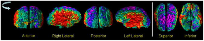
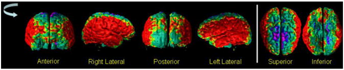
Fig.7. Cortical Thickness In Images Reconstructed from Maps of Relaxation Times for a Healthy Adult.

Using T1-weighted image and maps of T1 and T2 relaxation times for a healthy adult, we generated maps of relaxation times at various ages by varying the T1 relaxation times and water content with age. We then applied either the histogram-based or the MRF-based methods for tissue segmentation and generated the voxelwise (Rows One and Two) and surface maps (Rows Three and Four) of difference in the cortical thickness at increasing age compared to the cortical thickness at age 20 years. The bottom row shows the various views of the surface plot as the brain in rotated anticlockwise and the views from the superior and inferior directions. The difference in the cortical thickness was color encoded using the coding in Fig.2. These maps showed that the decrease in cortical thickness was regionally specific, with bilateral decrease in the prefrontal cortex, posterior and inferior parietal cortex, and the cerebellum, and with bilateral increases in thickness at the vertex of the brain. Cortical thickness increased at the vertex due to spatial variations in relaxation times across the brain.

Fig.8. Tissue Contrast and GM Voxels in the Cortex in Images Reconstructed Using Maps of Relaxation Times in a Healthy Adult.

The plots show differential change in relaxation times decreased percent tissue contrast, which in turn decreased the number of voxels labeled as GM. In addition, the rate of decrease in tissue contrast matched the rate of decrease in contrast measured empirically in our real-world sample of healthy participants (Fig.1). Thus, changes in relaxation times alone can account for the previously reported, age-related decline in cortical thickness.

3.2 Differences in Tissue Contrast Between Healthy Individuals and Individuals with Psychiatric Illnesses

3.2.1 Tissue Contrast and Cortical Thickness in SZ Adults

Tissue contrast decreased 0.0485 each year in our sample of 74 adults with SZ (Fig.9). Modeling tissue contrast as the dependent variable in a multiple linear regression and with age, gender, and diagnosis as independent variables, contrast for the SZ group was significantly higher than for healthy adults (41.18±2.04 vs 40.17±1.47, respectively, P-value < 0.05, df = 116, for Student's t-test). Our prior findings suggest that the greater tissue contrast, in turn, should yield a thicker cortex in the SZ compared with HC group, especially in the lateral and inferior surfaces of the brain, and thinner surfaces along the dorsal aspect of the parietal lobe. Consistent with this prediction, cortical thickness measured in the SZ group was greater along the lateral and inferior surfaces of the brain and thinner in the superior parietal lobe (Fig.10).

Fig.9. Tissue Contrast in Healthy Participants and Persons with Schizophrenia (SZ).

In our sample of 46 healthy adults (HA) and 74 adults with SZ, a plot of percent tissue contrast with age showed that the T1-weighted images for SZ adults had higher tissue contrast compared to the images for the healthy adults. After controlling for age and sex using multiple linear regression, the contrast in SZ brains was higher by 1.03 (p < 0.05) than the healthy brains. In addition, the percent contrast decreased at a rate of −0.035 per year, which was statistically significant (P-value = 0.031). We computed contrast by using the average GM and WM tissue intensities and therefore the tissue contrast is largely invariant to the random scanner noise. Because the MR images were acquired on the same MRI scanner with identical pulse sequences, the variations in tissue contrast across participants are primarily due to physiological variations in the brain across participants. The variations in scanner characteristics and noise will have only a small influence on measurement variations in tissue contrast. Furthermore, the linear fit best explains the change in contrast with age both visually and our derivations that predicted a linear relation between change in tissue contrast and relaxation times. The rate of change in contrast was less than that in our other cohort of healthy participants (Fig.1) because they were older than the healthy adults of our cohort.

HA=Healthy Adult; SZ=Schizophrenia

Fig.10. The Surface Maps of Differences in Cortical Thickness Between SZ Adults and Healthy Adults.

We compared cortical thickness in our cohort of 46 healthy adults to those of 74 adults with Schizophrenia (SZ), while controlling for the effects of gender and whole brain volume. The P-values of the differences in the cortical thickness were color encoded and displayed on the surface of the brain. Red and yellow color indicated significant (P-value < 0.05) increases and purple and blue indicate significant decreases (P-value < 0.05) in cortical thickness of SZ adults. These maps indicated that SZ adults had thicker cortex in the lateral aspects and thinner cortex in the superior parietal regions of the brain. The thicker cortex in SZ adults were expected because the SZ adults had higher tissue contrast (Fig.9) than healthy adults and because our previous results had shown that the automated methods defined thicker cortex in images with higher tissue contrast (Figs. 2, 5, & 7). In addition, the spatial pattern of the between-group differences in thickness matches the spatial pattern of change in thickness with decreasing tissue contrast (Fig.7), thereby suggesting that the differences in between-group tissue contrast at least confounded the between-group differences in cortical thickness.

HA=Healthy Adult; SZ=Schizophrenia

3.2.2 Tissue Contrast and Cortical Thickness in Persons with BD

Tissue contrast in images from BD participants did not vary with age (Fig.11), but they were significantly higher than that in images for healthy adults (40.27±1.04 versus 38.9±1.17, P-value<0.000001, df = 84). Because tissue contrast in the BD group was higher than in age-matched HCs, we expected that automated segmentation would yield thicker cortices in the BD group, as suggested by findings in our synthetic datasets. Consistent with this prediction, cortical thickness in the BD group was significantly greater across most of the brain, with some thinning noted in superior parietal regions (Fig.12), suggesting that greater tissue contrast contributed to the thicker cortices measured in the BD group.

Fig.11. The Change in Tissue Contrast With Age.

in our cohort of 52 healthy participants (HA; 25 males, age 27.71±14.1 years) and 36 participants with Bipolar Disorder (BD; 17 males, age 31.38±14.67 years). Using multiple linear regression to control for age, gender, and diagnosis, the percent contrast was higher by 1.24 in BD participants as compared to the healthy participants (P-value = 1.07 * 10⁻⁶). And similar to the SZ participants, the contrast did not differ (P-value = 0.3155) between males and females in this cohort of participants. Furthermore, although the percent contrast decreased at a rate of -0.012 per year for BD participants, the decrease in contrast was not statistically significant (P-value = 0.34). However, within healthy participant, the decrease in contrast with age was statistically significant (P-value = 0.0032). Purple Squares: Healthy Participants; Blue Diamonds: Participants with BD.

HA=Healthy Adult; BD=Bipolar Disorder

Fig.12. The Maps of Difference in Cortical Thickness Between Healthy Participants and Participants with Bipolar Disorder (BD).

In our cohort of 52 healthy adults (HA) and 36 participants with Bipolar Disorder (BD) we computed cortical thickness. At each point on the template surface, we used multiple linear regression to correlate cortical thickness with diagnosis while controlling for the age and gender effects. The P-values were color encoded and displayed on the surface, with red and yellow showing thicker cortex and purple and blue showing thinner cortex in BD participants. These maps showed that bilaterally the BD participants had thicker cortex in the lateral aspect and thinner cortex in the vertex of the brain. The spatial pattern of the differences in cortical thickness matched the spatial pattern of the change in cortical thickness with tissue contrast (Fig.7) and was similar to the spatial pattern of differences in thickness between adults with Schizophrenia (SZ) and healthy adults (Fig.10). The BD participants had higher tissue contrast as compared to the age- and sex-matched healthy participants (Fig.13), thereby suggesting the observed differences in the thickness in BD participants compared to the healthy participants.

HA=Healthy Adult; BD=Bipolar Disorder

3.2.3 Correlating Cortical Thickness with Tissue Contrast

Cortical thickness averaged across the entire cerebral surface correlated significantly with average tissue contrast for the BD participants (Pearson's r = 0.277, p< 0.05) and for the healthy participants (Pearson's r = 0.24, p = 0.04) (Fig.13). The maps of correlation of tissue contrast with cortical thickness at each point across the surface of the brain showed large expanses of positive correlations between cortical thickness and contrast for BD and healthy participants (Fig.14). For SZ participants, however, average cortical thickness did not correlate significantly with the tissue contrast (Pearson's r = 0.0077, p=0.474), and correlation maps showed regions with both positive and negative correlations between tissue contrast and cortical thickness (Fig.14). These regional positive and negative correlations cancel one another in the average and explain why average cortical thickness across the entire brain did not correlate significantly with tissue contrast in the SZ group (Fig.13).

Fig.13.

The Change in Average Cortical Thickness with Tissue Contrast in our cohort of 52 healthy adults (HA) and 36 participants with Bipolar Disorder (BD). We computed the average cortical thickness in the participant brains that were not scaled for the whole brain volumes and segmented the brain tissue as gray matter (GM) and white matter (WM) using the automated method based on histogram of tissue intensity. These plots showed that the average cortical thickness was significantly correlated (BD: Pearson r = 0.277, P-value = 0.046; HA: Pearson r = 0.24, P-value = 0.043) with tissue contrast. In addition, BD participants had thicker cortex (P-value = 0.015) and higher tissue contrast (P-value = 1.07 * 10⁻⁶) compared to the healthy participants.

HA=Healthy Adult; BD=Bipolar Disorder

Fig.14. The Maps of Change in Cortical Thickness with Tissue Contrast.

while controlling for the effects of sex. We applied multiple linear regression at each point on the surface of the brain with the cortical thickness as the independent variable and the tissue contrast and sex as the independent variables. Age was not used as an independent variable because it correlated significantly with contrast (Fig. 1). We generated these color maps independently for the 38 participants with Bipolar Disorder (BD, Top Row), 58 healthy participants (Middle Row), and 74 adults with Schizophrenia (SZ, Bottom Row). The P-value maps were controlled for false positive due to multiple comparisons by applying a method for False Discovery Rate (FDR) with the false discovery rate set at 0.05. These maps showed that although there were few localized brain regions with negative associations, especially in the adults with SZ, in general changes in cortical thickness were positively associated with tissue contrast. Thus, automated tools for tissue segmentation defined thicker cortex in brain images with higher tissue contrast in each of our three independent sets of brains from healthy participants, participants with BD, and adults with SZ.

SZ = Schizophrenia; BD = Bipolar Disorder

4. Discussion

We have shown that T1-weighted MR images with lower tissue contrast yield thinner measures of the cerebral cortex. We have also shown that age-related changes in relaxation times of GM and WM produce a progressive decline in tissue contrast with age and that this change in contrast in turn yields measures of cortical thickness that decline with age. This age-related decline in cortical thickness does not represent what would be measured for thickness of the cortical mantle ex vivo, but rather is a product solely of changing relaxation times in GM and WM with advancing age. We have furthermore shown that subtle declines in water content of GM and WM with age likely account in large part for the age-related changes in relaxation times and declines in both tissue contrast and measures of cortical thickness with age. Finally, we have shown that differences in tissue contrast across groups patients and healthy controls contributes significantly to differences in cortical thickness measured across groups. We conclude that the changes in cortical thickness across ages and the differences in cortical thickness across diagnostic groups reported extensively in the literature are attributable at least in part to differences in tissue contrast across ages and diagnostic groups. Those group differences in tissue contrast by definition derive, in turn, from group differences in the cellular and molecular properties of GM and WM tissue, including their water content, not from true underlying differences in thickness of the cortical mantle.

A decline in water content with age produces changes in relaxation times for GM and WM that reduce tissue contrast progressively with age, and this age-related decline in tissue contrast in turn produces a progressive, age-related thinning of the cortex. We derived analytic relations associating changes in T1 and T2 relaxation times in GM and WM with changes in tissue intensities and contrast in T1-weighted images of the brain. Using previously reported, age-specific values for relaxation times, these analytic relations predicted decreases in tissue contrast with age that we confirmed in our real-world cohort of healthy participants. In addition, we showed analytically that more GM voxels are misclassified as WM voxels for declining values of tissue contrast. GM voxels along the interface of GM and WM should be the most misclassified as WM, because those are the GM voxels with the highest tissue intensities because of the presence of partial volume effects. Misclassification of GM as WM at locations of GM/WM interface will produce a progressive thinning of the cortex with progressively declining tissue contrast.

We experimentally assessed the effects of tissue contrast on the segmentation of the cortex using three sets of computer-generated images and two sets of real-world data from healthy and patient participants. The computer-generated images in the three simulated datasets modeled the real-world change in tissue contrast with increasing accuracy and complexity: In the first set, images increased GM intensities solely to reduce tissue contrast at a rate that we observed in our real images of healthy adults. In the second set, we reconstructed T1-weighted images from synthetic maps of T1 and T2 relaxation times in GM and WM reported previously at specific ages. In the third set, we reconstructed T1-weighted images from maps of relaxation times measured in a healthy adult and varying those measures by the values for T1 and T2 reported previously for specific ages. Tissue contrast in the T1-weighted images reconstructed from the maps of relaxation times in both the second and the third datasets declined with age, as expected from both our empirical data and as predicted by the analytic relations we derived between relaxation times and tissue contrast. We segmented brain tissues in each of the three datasets and in the real-world cohorts using both histogram- and MRF-based methods for segmentation and showed that although tissue contrast decreased by only 3-4%, cortical thickness and the number of voxels labeled as GM declined by more than 15% over the human lifespan. Furthermore, MRF-based segmentation generated thinner cortical measures than did histogram-based segmentation (Fig.5).

Images reconstructed from maps of relaxation times in a single individual that were then varied synthetically using previously reported relaxation times at specific ages showed regions of age-related thinning and thickening of the cortex bilaterally, which we also observed in our real-world cohort of healthy participants. In these healthy participants, those with lower tissue contrast had proportionally thinner cortices. These same associations between tissue contrast and cortical thickness were observed in our group comparisons of patients with age-matched healthy controls. For example, tissue contrast was greater and cortical thickness proportionally greater in SZ compared with healthy participants (Fig.10) in BD compared with healthy control participants (Fig.12) in regionally specific patterns consistent with those observed for the effects of age on contrast and cortical thickness. These regionally specific differences in thickness across diagnostic groups were likely caused by regionally specific differences across groups in relaxation times,¹⁴ which in turn likely depended on regional variation across groups in water content and other cellular properties of the tissue, rather by group differences in underlying thickness of the cortical mantle.

4.1 Corroboration and Internal Consistency of Our Findings

Several independent observations support our thesis that tissue contrast in T1-weighted images of the brain decreases with increasing age and that its effect on tissue segmentation is responsible for age-related cortical thinning.

1. We analytically derived the equations that linearly relate the change in tissue intensities and the change in tissue contrast with the changes in T1 relaxation times and water content of GM and WM. With increasing age, T1-relaxation times decline in GM and increase in WM, thereby reducing tissue contrast. Although the change in tissue contrast relates linearly to the change in relaxation times, relaxation times may possibly change nonlinearly with age and therefore may produce nonlinear, age-related decreases in tissue contrast.

2. We derived the analytic relation showing that changing tissue contrast yields misclassification of GM and WM voxels that affects each tissue type in equal proportions. Nevertheless, the greater number of GM voxels in the brain leads to misclassification of a greater number of GM than WM voxels, so that declining tissue contrast produces an apparent overall decline in GM tissue.

3. The rate of age-related decline in tissue contrast observed empirically in a sample of healthy adults (Fig.1) matched closely the rate of age-related decline in tissue contrast that were detected in computer-generated images constructed from maps of relaxation times measured in a healthy adult participant and modified using age-specific relaxation times and proton densities reported in prior studies (Fig.8). We showed that age-related changes in water content is largely responsible for age-related changes in proton density and relaxation times, and that therefore age-related changes in water content is also likely responsible for real-world, age-related changes in tissue contrast.

4. The regional pattern of age-related change in cortical thickness in T1-weighted images reconstructed from the age-specific maps of relaxation times matched well the previously reported, regional pattern of age-related changes in cortical thickness. Cortical thickness in both instances declined linearly with age in frontal, superior temporal, and lateral parietal cortices^49-52 and changed little with age in ventral portions of the brain.^{49, 53, 54}

5. In two independent samples of patient and healthy participants, group differences in tissue contrast accounted for group differences in measured cortical thickness (Figs.10 & 12). Moreover, the regional pattern of these group differences in cortical thickness (Figs.10 & 12) matched well the regional pattern of cortical thinning associated with age-related changes in tissue contrast that we observed in our synthetic datasets (Fig.7). These findings suggest that group differences in tissue contrast, and therefore group differences in water content and other cellular or molecular characteristics of the underlying tissue, rather than real differences in underlying thickness of the cortical mantle, likely was responsible for the observed differences across groups in imaging-based measures of cortical thickness.

6. The previously reported, age-related decline in cortical thickness matches well the age-related decline in thickness that we observed in our computer-generated images. One prior study reported a 15-20% reduction in cortical thickness uniformly across the brain of healthy participants between the ages of 10 and 90 years.^{55, 56} Another reported a decline in GM volume of either 9.2% (corrected for total intracranial volume) or 14.3% (uncorrected for total intracranial volume) over 40 years in healthy adults⁵⁷. The magnitude of these in vivo, age-related changes in GM agrees well with the magnitude of age-related changes in GM measured in our computer-generated images.

7. Previous studies^{36, 76} have also reported larger age-related changes in the gray-scale intensities of WM than GM. We established these same tissue-specific changes in gray-scale intensity analytically in the relation of changing tissue intensity, relaxation times, and water content of brain tissue, and we observed the same changes in our computer-generated images that modeled relaxation times using previously published values at differing ages.

8. Although we evaluated the effects of two automated methods for tissue segmentation on our measures of cortical thickness, prior studies that have used other segmentation methods, such as FreeSurfer,^58-60 have also reported thinner cortices in images with lower tissue contrast^{50, 51}, and in regions similar to those where we detected cortical thinning specifically associated with reduced contrast.

4.2 Changes in Tissue Contrast Associated with Changes in Water Content

We believe that age-related changes in tissue intensity and tissue contrast derive primarily from age-related changes in water content of the brain. Water content declines rapidly from 95% of brain weight at birth to about 81% at 1 year of age⁶¹. It continues to decrease slowly with age thereafter, especially in gray matter.¹⁵ The rapid changes in water content immediately after birth alters relaxations times and thereby causes rapid changes in tissue intensities and tissue contrast in MR images. In fact, the changes in water content cause the difference in T1 and T2 relaxation times for GM and WM, and therefore the tissue contrast that depends on those relaxation times, to invert at approximately 3 months of age. Thus the underlying morphological features of brain tissue have changed relatively little compared to the very dramatic change in the brain's appearance on MR images around 3 months of age.⁶² Although other cellular and molecular properties of brain tissue change with age,⁶³ these are thought to produce relatively small changes in relaxation times compared with the dramatic effects that changing water content has on relaxation times and tissue intensities. ^{63,64,65, 66}. Thus, we contend that the differential change in the water content of GM and WM with age in healthy individuals largely drives the changes in tissue intensities and contrast with increasing age and therefore likely also drives the effects that changing contrast has on age-related changes in measures of cortical thickness in MR images.

4.3 Variance in Tissue Contrast Across Individuals

The variance in brain tissue contrast (Figs. 9, 11, & 13) across participants in scans acquired using identical pulse sequence parameters is caused by individual differences in brain chemistry that alters their T1 and T2 relaxation times (Appendix A), as well as partial volume effects and noise in the acquisition and reconstruction of the MRI data. Variation in relaxation times and tissue contrast in a single participant across time derives from these same sources as well as from physiological changes in the brain, which include changes in the tissue water content. To demonstrate that the age-related variance in tissue contrast that we are studying is not likely caused by partial volume effects or noise in image acquisition and reconstruction, and therefore is likely caused primarily by age-related changes in physiology and water content, we measured tissue contrast in a cohort of 10 healthy young adults (9 females, ages 12.03 to 17.76 years) for whom we had acquired two brains scans 3 months apart on a 3T MR scanner. We expected minimal physiological change in the brain over a 3-month period in each participant and therefore we would attribute any variations observed in individual scans to errors in measurement of contrast that derived from variations in scanner performance, noise in image acquisition and reconstruction, and inaccuracies in measurement of tissue contrast in the images. Because within individual variance in repeated measures are expected to be small, the large variance across individuals would therefore be due to physiological differences across brains. As we expected, although tissue intensities in the brains across the two time points were not correlated (Pearson r=0.07, P-value=0.86), measures of tissue contrast correlated strongly and significantly within the same brains across time points (Pearson r=0.94, P-value = 1.42 × 10⁻⁵) (Fig. 15). Variation across time was minimal compared with the variance in contrast across individuals and across ages. We therefore conclude that the large variance in contrast across individuals and across ages in our study derived from physiological differences across brains and not from noise or measurement error.

Fig.15. Gray Matter Intensities and Percent Tissue Contrast Measured in the Same Individuals at Two Time Points.

We measured and plotted the average gray matter (GM) intensities and the percent tissue contrast in the brains of 10 participants (9 females, age range 12.03 to 17.76 years) for whom we acquired two scans at a 3-month interval. Although the tissue intensities were not correlated (Pearson r=0.07, P-value=0.86) at the two time points, the percent contrasts were nearly perfectly correlated (Pearson r=0.94, P-value=1.42 × 10⁻⁵) across time, differing by less than 5% within participants. For a single individual, possible sources of variance across time points included (1) changes in scanner characteristics, including amplifier gain, over time, (2) noise in the imaging data, and (3) changes in the brain physiology over the three-month interval between scans (which seems highly unlikely). The younger adolescents (ages 12.03 to 14.4 years) had a higher percent contrast (>81), whereas the older adolescents (ages (14.88 to 17.76 years) had a lower percent contrast (<75) at both time points, as we had expected. Furthermore, this plot demonstrated that tissue contrast can differ across individuals of similar ages by more than 30% based on physiological differences (the average Time1 contrast was 76.12±8.05). Because tissue contrast depends only on relaxation times, we surmise that relaxation times vary across individuals because of physiological differences in their brains.

4.4 The Potential Confounding Effects of Changing Water Content on Brain Imaging Measures

Several imaging studies have shown that tissue contrast differs in patient populations compared with healthy participants. We suspect that these group differences in tissue contrast may be caused by subtle differences in water content of the brains across these diagnostic groups. Changes in water content have been associated with specific neuropathological conditions, including cerebral haematoma, stroke, brain tumors, and hepatic encephalopathy.^{17, 67-69} In psychiatric illnesses, group differences in water content may be more subtle, but their possibility is supported by reports that tissue contrast is reduced in patients with schizophrenia⁵⁰ and Alzheimers disease⁵¹. We have shown that reductions in water content reduce tissue contrast, which in turn reduces measures of GM. We have shown, similar to other reports, that patient groups can differ in their tissue contrast, and we further showed that those group differences in tissue contrast account for group differences in measures of cortical thickness. Therefore, we suspect that the group differences in GM measures frequently reported in patient populations may derive in large part from differences in tissue contrast, and that those differences in tissue contrast derive in turn from group differences in water content of the tissues.

Thus, even though thinning of the cortex has been almost universally presumed to represent the effects of synaptic or dendritic pruning or increasing myelination of adjacent white matter⁷⁰, it may instead represent differential changes in water content of the GM and WM and its effects on tissue contrast, rather than true underlying differences in thickness of the cortical mantle. Many processes can potentially alter the local water content of brain tissue, including changes in glial cells or microvasculature⁷¹, intracortical myelination⁷², tissue perfusion, and fat deposition. Steroids⁷³ and other hormones⁷⁴, alcohol⁷⁵, and lithium treatment⁷⁶ all cause rapid changes in tissue permeability and water content of the brain, and they produce measurable and reversible⁷⁷ changes in MR images over only a few week's time. Because 80% of brain volume consists of water, MR signal intensity and tissue contrast are more sensitive to changes in water content than to most other changes in brain tissue, and thus subtle changes in water content with age and in illness could produce the previously reported prominent effects of age and diagnosis on brain imaging measures.

4.5 Age-Related Changes in Brain Volume and Water Content in Healthy Participants

Our empirical data in healthy adult participants showed that about 60% of the brain is gray matter and 40% white matter (Fig.15) and that from age of 25 years to 65 years, whole brain volume (WBV) decreases overall by 2.9%, with GM volume decreasing by 9.78%, and WM volume increasing by 8.21% (Fig.16). These age-related changes in the volumes of each tissue type in healthy adults can be explained by the change in water content of GM and WM, without the concurrent loss of any neuropil or neurons with age. Here we provide some additional, simple calculations that support the plausibility of this assertion.

Fig.16. The Change in the Whole Brain Volume and Tissue Volumes with Age.

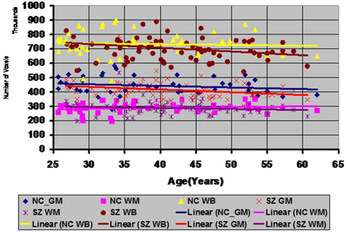
in healthy adults and adults with SZ. We applied the histogram-based method to segment the brain as gray matter (GM) and white matter (WM) in our cohort of 46 healthy adults (HA) and 74 adults with Schizophrenia (SZ). These plots showed that from age 25 years to age 65 years in healthy adults the WBV decreased by 2.9% (yellow triangles, Pearson r = −0.06 P-value = 0.35), the GM volume decreased by 9.78% (blue diamonds, , Pearson r = −0.173, P-value = 0.125), and the WM volume increased by 8.21% (purple squares, , Pearson r = 0.156, P-value = 0.148). In SZ adults, the WBV decreased by 14.05% (brown circles, Pearson r = −0.215, P-value = 0.033), the GM volume decreased by 16.9% (red cross, Pearson r = −0.247, P-value=0.017), and the WM volume decreased by 9.69% (violet cross, Pearson r = −0.13, P-value = 0.13). Although in healthy adults the volumes did not change significantly with age, similar to other reported studies⁵⁷, volume changes may not be significant because of small age range (40 years from age 25 years to age 65 years) and because brain maturation due to developmental changes are typically completed by the second decade of life. Yet, the data showed that at age 25 years the WBV of adults with SZ matched the WBV of healthy adults and that for healthy adults the WBV decreased by 2.9% over the period of 40 years, which was close the 4.5% decrease in WBV in another study⁷⁸ for the same age range in healthy adults.

HA=Healthy Adult; SZ=Schizophrenia

In healthy adults, water content between 25 and 60 years of age declines from 81% to 79% in GM and increases from 70% to about 72% in WM.¹⁵ Assume, for the sake of illustration, that the entire brain consists of 100 voxels, with 60 voxels belonging to GM and 40 voxels to WM. Then, assuming only water content in each tissue compartment changes from age 25 to 65 years, we calculate GM and WM volumes at each of those ages:

• GM at age 25 years: with 81% water content in GM at age 25, water occupies roughly 48.6 GM voxels and non-water tissue occupies 11.4 GM voxels.

• WM at age 25 years: with a 70% water content in WM, water occupies 28 WM voxels and non-water tissue occupies 12 WM voxels.

If only water content were to change with age, then the volumes of each tissue component at age 65 are as follows:

• GM at age 65 years: with 79% water content in GM at age 65, water occupies 42.88 GM voxels, and non-water tissue occupies 11.4 GM voxels, for a total of 54.28 GM voxels.

• WM at age 65 years: with 72% water content, water occupies 30.85 WM voxels and non-water tissue occupies 12 WM voxels, for a total of 42.85 WM voxels.

• (Note that we can reverse these calculations of volumes of non-water tissue from known water content to estimate water content from known brain volumes, and below we do so in estimating water content in the brains of our SZ and BP samples.)

At age 65 years, therefore, WBV comprises 97.13 (=54.28 GM+42.85 WM) voxels. Assuming that only water content had changed since the age of 25 years, WBV would have decreased by 2.9% (from 100 to 97.1 voxels), GM volume would have decreased by 9.53% (from 60 to 54.28 voxels), and WM volume would have increased by 7.125% (from 40 to 42.85 voxels).

Note that these volume changes in WBV and in the volumes of GM and WM tissue compartments, which were calculated solely on the basis of the known, previously reported changes in water content of the brain, account almost entirely for all of the change in WBV, GM, and WM that we observed empirically in our sample of healthy adult participants. Thus, these simple calculations suggest convincingly that changing water content -- and not the commonly assumed loss of neurons, synaptic density, neuropil, or glial cells -- is the primary determinant of empirically observed changes in volumes of GM and WM with age.

4.6 Altered Tissue Contrast and Possible Differences in Water Content in Individuals with Schizophrenia

The higher tissue contrast that we observed in persons with SZ suggests the possibility of higher water content in their brains. Although we did not directly measure water content in these participants, we can estimate water content from tissue volumes by reversing the steps that we used above to estimate tissue volumes from known water content in healthy adults. From age 25 to 65 years in our SZ participants, WBV decreased by 14.05%, GM volume decreased by 16.9%, and WM volume decreased by 9.69% (Fig.16). We assume that water content at age 25 years is similar in SZ and healthy adults (i.e., 81% in GM and 70% in WM), given that WBV across groups is similar for participants at that age (Fig.16). We also assume that the loss in tissue volume in the SZ group was caused only by reduction in water content, then by age 65 years the water content would decline in GM to 77.14% and in WM to 66.78%. Therefore, by age 65 years, the SZ group would have 2% less water content in GM and 5% less water content in WM compared with healthy control participants. Therefore, reduced water content in the brains of SZ adults would have reduced WBV but it would also have produced a differential change in the water content of GM and WM, which would have increased tissue contrast in the SZ group. Both the scaling of the SZ brains to match a template brain and the greater tissue contrast in the SZ group contributed to measures of cortical thickness that were greater in the SZ sample.

4.7 Altered Tissue Contrast and Possible Differences in Water Content in Individuals with Bipolar Disorder

Similar to the SZ participants, those with BD had higher tissue contrast than their age-matched healthy peers (Fig.11), and therefore we expected BD participants to have thicker cortices along the lateral surface of their brains and thinner cortices in superior parietal regions. This pattern of regional differences was confirmed statistically in the BD group (Figs. 7 & 12). We used procedures identical to those for the SZ group to estimate differences in water content of the brains of the BD participants that would be required to account for the change in tissue volumes if those volume differences were attributable to the effects of altered water content alone. Between the ages 10 and 60 years in the BD participants, WBV declined by 9.95%, GM volume decreased by 18.99%, and WM volume increased by 4.36% (Fig.17). We assume that at age 10 years water content in the brains of the BD participants was similar to the healthy participants, as their WBVs were similar to those in healthy participants. Assuming also that group differences in tissue volumes were caused solely by group differences in water content, then water content would change from 81% in GM and 70% in WM at age 10 years to 76.5% in GM and 71% in WM at age 60 years. Therefore, although GM water content was lower in the BD compared with healthy group at age 60 years, the WM water content at age 60 was similar across groups. Thus, a differential age-related change in water content of GM and WM could have accounted for the greater tissue contrast in the T1-weighted images of the BD group, which in turn could account for the thicker cortices measured in that group.

Fig.17. The Change in Tissue Volumes with Age of Participants with Bipolar Disorder (BD).

We isolated the brain in T1-weighted images and labeled the brain tissue as gray matter (GM) or white matter (WM) by applying the histogram-based method for segmentation. From age 10 years to age 60 years, the whole brain volume (WBV) decreased by 9.95% (red crosses, Pearson r = -0.242, P-value = 0.07), the GM volume decreased by 18.99% (yellow triangles, Pearson r = -0.4338, P-value = 0.0032), and the WM volume increased by 4.36% (brown circles, Pearson r = 0.0724, P-value = 0.3328). Although the Pearson correlation for the increase in WM volume was small and therefore not statistically significant, the volumes of GM and WM decreased significantly with age.

4.8 The Effects of Tissue Contrast on Subcortical Brain Regions

Although we investigated the effects of tissue contrast on the definition of the cerebral cortex only, changes in tissue contrast will also affect the definition of subcortical regions. Longitudinal and transverse relaxation times differ from one brain region to another¹⁴ and may change nonlinearly with age³¹. We expect that tools for automated tissue segmentation, similar to their effects in cortex, will generate reduced volumes of subcortical gray matter regions in images with lower tissue contrast. In fact, our synthetic images reconstructed from the maps of relaxation times for the healthy participant showed loss of subcortical gray matter with age, especially when the brain tissue was segmented using the MRF-based method (Fig.5). Therefore, In addition to scaling by WBV, incorporating tissue contrast as an independent variable in multivariate statistical techniques would help to ensure that between-group findings are associated with true underlying morphological and cellular processes rather than to the effects of differing tissue contrast. On the other hand, if the underlying pathological processes alter water content and therefore also change tissue contrast, then covarying for tissue contrast in these statistical procedures would covary out the effects of the pathological processes. Thus, disentangling the effects of altered water content, relaxation times, and tissue contrast from true underlying cellular and pathological processes is challenging and must be undertaken with caution and care.

4.9 Conclusion

We demonstrated that changes in certain tissue properties can profoundly influence in vivo measures of brain morphology computed using anatomical MR images, properties that may not have any effects on the ex vivo measures derived from histological analyses of the tissue. The water and the iron content of brain tissue are some of the tissue properties that may have the largest influence on the in vivo measures and their variance with age and across brain regions. In particular, because water content of brain tissue largely determines MR signal, variations in water content across individuals, and within individuals across time, is a powerful determinant of the variability in relaxation times across the brain. Differential change in relaxation times with age in gray matter and white matter will change tissue contrast, and change it in regionally specific way across the brain. These changes in tissue contrast, which has little or nothing to do with the molecular and cellular properties of the tissue, may have profound influences on the morphological measures derived from MR images of the brain. By deriving mathematical relations and computer-generated and real-world imaging data of participants with various neuropsychiatric illnesses, we demonstrated that differential variations of water content in GM and WM account for important differences in morphological measures across age and across diagnostic groups. These morphological variations caused solely by tissue properties unrelated to underlying cellular and morphological features of the tissue will cause misinterpretation of imaging findings, thereby generating invalid inferences for normative development of the brain in healthy individuals and for the localized disturbances in the brains of individuals with neuropsychiatric illnesses. Thus, because tissue contrast may differ systematically between groups of participants, and because tissue contrast changes with age, imaging studies that aim to define normal brain development or identify the anatomical disturbances associated with psychiatric illness must develop and incorporate methods to control for the effects that systematic variations in tissue contrast have on imaging measures.

References

- 1.Hallgren B, Sourander P. The Effect of Age on the Non-Haemin Iron in the Human Brain. Journal of Neurochemistry. 1958;3(1):41–51. doi: 10.1111/j.1471-4159.1958.tb12607.x. [DOI] [PubMed] [Google Scholar]
- 2.Bottomley PA, Foster TH, Argersinger RE, Pfeifer LM. A Review of Normal Tissue Hydrogen NMR Relaxation-Times and Relaxation Mechanisms from 1-100 Mhz - Dependence on Tissue-Type, NMR Frequency, Temperature, Species, Excision, and Age. Medical Physics. 1984;11(4):425–448. doi: 10.1118/1.595535. [DOI] [PubMed] [Google Scholar]
- 3.Rooney WD, Johnson G, Li X, et al. Magnetic field and tissue dependencies of human brain longitudinal 1H20 relaxation in vivo. Magnetic Resonance in Medicine. 2007 Feb;57(2):308–318. doi: 10.1002/mrm.21122. [DOI] [PubMed] [Google Scholar]
- 4.Powchik P, Davidson M, Haroutunian V, et al. Postmortem studies in schizophrenia. Schizophrenia Bulletin. 1998;24(3):325–341. doi: 10.1093/oxfordjournals.schbul.a033330. [DOI] [PubMed] [Google Scholar]
- 5.Chance SA, Esiri MM, Crow TJ. Amygdala volume in schizophrenia: post-mortem study and review of magnetic resonance imaging findings. British Journal of Psychiatry. 2002 Apr;180:331–338. doi: 10.1192/bjp.180.4.331. [DOI] [PubMed] [Google Scholar]
- 6.Gigante AD, Young LT, Yatham LN, et al. Morphometric post-mortem studies in bipolar disorder: possible association with oxidative stress and apoptosis. International Journal of Neuropsychopharmacology. 2011 Sep;14(8):1075–1089. doi: 10.1017/S146114571000146X. [DOI] [PubMed] [Google Scholar]
- 7.Vawter MP, Freed WJ, Kleinman JE. Neuropathology of bipolar disorder. Biological Psychiatry. 2000 Sep 15;48(6):486–504. doi: 10.1016/s0006-3223(00)00978-1. [DOI] [PubMed] [Google Scholar]
- 8.Kapur T, Grimson WE, Wells WM, 3rd, Kikinis R. Segmentation of brain tissue from magnetic resonance images. Med Image Anal. 1996 Jun;1(2):109–127. doi: 10.1016/S1361-8415(96)80008-9. [DOI] [PubMed] [Google Scholar]
- 9.Zhang Y, Brady M, Smith S. Segmentation of brain MR images through a hidden Markov random field model and the expectation-maximization algorithm. IEEE Trans Med Imaging. 2001 Jan;20(1):45–57. doi: 10.1109/42.906424. [DOI] [PubMed] [Google Scholar]
- 10.Alfano B, Brunetti A, Covelli EM, et al. Unsupervised, automated segmentation of the normal brain using a multispectral relaxometric magnetic resonance approach. Magn Reson Med. 1997 Jan;37(1):84–93. doi: 10.1002/mrm.1910370113. [DOI] [PubMed] [Google Scholar]
- 11.Collins DL, Zijdenbos AP, Baare WFC, Evans AC. ANIMAL+INSECT: Improved cortical structure segmentation. Information Processing in Medical Imaging, Proceedings. 1999;1613:210–223. [Google Scholar]
- 12.Ashburner J, Friston KJ. Unified segmentation. NeuroImage. 2005 Jul 1;26(3):839–851. doi: 10.1016/j.neuroimage.2005.02.018. [DOI] [PubMed] [Google Scholar]
- 13.Rivest-Henault D, Cheriet M. Unsupervised MRI segmentation of brain tissues using a local linear model and level set. Magn Reson Imaging. 2011 Feb;29(2):243–259. doi: 10.1016/j.mri.2010.08.007. [DOI] [PubMed] [Google Scholar]
- 14.Oros-Peusquens AM, Laurila M, Shah NJ. Magnetic field dependence of the distribution of NMR relaxation times in the living human brain. Magnetic Resonance Materials in Physics Biology and Medicine. 2008 Mar;21(1-2):131–147. doi: 10.1007/s10334-008-0107-5. [DOI] [PubMed] [Google Scholar]
- 15.Neeb H, Zilles K, Shah NJ. Fully-automated detection of cerebral water content changes: Study of age-and gender-related H2O patterns with quantitative MRI. NeuroImage. 2006 Feb 1;29(3):910–922. doi: 10.1016/j.neuroimage.2005.08.062. [DOI] [PubMed] [Google Scholar]
- 16.Kugel H, Roth B, Benz-Bohm G, Heindel W, Lacker K. The Water Content of Brain Tissue in Infants Determined Using MR Imaging: The Internal Reference of Quantitative MR spectroscopy. ISMRM. 1999 [Google Scholar]
- 17.Andersen C. In vivo estimation of water content in cerebral white matter of brain tumour patients and normal individuals: Towards a quantitative brain oedema definition. Acta Neurochirurgica. 1997;139(3):249–255. doi: 10.1007/BF01844760. [DOI] [PubMed] [Google Scholar]
- 18.Hwang D, Kim DH, Du YPP. In vivo multi-slice mapping of myelin water content using T2* decay. NeuroImage. 2010 Aug 1;52(1):198–204. doi: 10.1016/j.neuroimage.2010.04.023. [DOI] [PubMed] [Google Scholar]
- 19.Ding XQ, Kucinski T, Wittkugel O, et al. Normal brain maturation characterized with age-related T2 relaxation times: An attempt to develop a quantitative imaging measure for clinical use. Investigative Radiology. 2004 Dec;39(12):740–746. doi: 10.1097/00004424-200412000-00005. [DOI] [PubMed] [Google Scholar]
- 20.Mansfield P, Morris PG. NMR Imaging in Biomedicine. Advances in Magnetic Resonance. 1982:1–343. [Google Scholar]
- 21.Papademetris X, Jackowski M, Rajeevan N, Okuda H, Constable RT, Staib LH. BioImage Suite: An integrated medical image analysis suite. Section of Bioimaging Sciences, Dept. of Diagnostic Radiology, Yale School of Medicine; Vol http://www.bioimagesuite.org. [Google Scholar]
- 22.Dale AM, Fischl B, Sereno MI. Cortical surface-based analysis. I. Segmentation and surface reconstruction. NeuroImage. 1999 Feb;9(2):179–194. doi: 10.1006/nimg.1998.0395. [DOI] [PubMed] [Google Scholar]
- 23.Ashburner J, Friston KJ. Unified segmentation. NeuroImage. 2005 Jul 1;26(3):839–851. doi: 10.1016/j.neuroimage.2005.02.018. [DOI] [PubMed] [Google Scholar]
- 24.Duda RO, Hart PE, Stork DG. Pattern classification. 2nd. New York: Wiley; 2001. [Google Scholar]
- 25.Kanungo T, Mount DM, Netanyahu NS, Piatko CD, Silverman R, Wu AY. An efficient k-means clustering algorithm: Analysis and implementation. IEEE Transactions on Pattern Analysis and Machine Intelligence. 2002 Jul;24(7):881–892. [Google Scholar]
- 26.Zhang YY, Brady M, Smith S. Segmentation of brain MR images through a hidden Markov random field model and the expectation-maximization algorithm. IEEE Transactions on Medical Imaging. 2001 Jan;20(1):45–57. doi: 10.1109/42.906424. [DOI] [PubMed] [Google Scholar]
- 27.Dempster AP, Laird NM, Rubin DB. Maximum Likelihood from incomplete data via EM algorithm. J Royal Statistical Soc, Ser B. 1977;39:1–38. [Google Scholar]
- 28.Moretti B, Fadili LM, Ruan S, Bloyet N, Mazoyer B. Phantom-based performance evaluation: application to brain segmentation from magnetic resonance images. Med Image Anal. 2000 Dec;4(4):303–316. doi: 10.1016/s1361-8415(00)00021-9. [DOI] [PubMed] [Google Scholar]
- 29.Sled GJ, Zijdenbos AP, Evans AC. A Nonparametric Method for Automatic Correction of Intensity Nonuniformity in MRI Data. IEEE Trans of Medical Imaging. 1998 Feb;17(1):87–97. doi: 10.1109/42.668698. [DOI] [PubMed] [Google Scholar]
- 30.Shattuck DW, Leahy RM. BrainSuite: An Automated Cortical Surface Identification Tool. Medical Image Analysis. 2002;8(2):129–142. doi: 10.1016/s1361-8415(02)00054-3. [DOI] [PubMed] [Google Scholar]
- 31.Suzuki S, Sakai O, Jara H. Combined volumetric T1, T2 and secular-T2 quantitative MRI of the brain: age-related global changes (preliminary results) Magnetic Resonance Imaging. 2006 Sep;24(7):877–887. doi: 10.1016/j.mri.2006.04.011. [DOI] [PubMed] [Google Scholar]
- 32.Rosenfel A, Pfaltz JL. Distance Functions on Digital Pictures. Pattern Recognition. 1968;1(1):33. [Google Scholar]
- 33.Rydberg JN, Riederer SJ, Rydberg CH, Jack CR. Contrast Optimization of Fluid-Attenuated Inversion-Recovery (Flair) Imaging. Magnetic Resonance in Medicine. 1995 Dec;34(6):868–877. doi: 10.1002/mrm.1910340612. [DOI] [PubMed] [Google Scholar]
- 34.Carneiro AAO, Vilela GR, de Araujo DB, Baffa O. MRI relaxometry: Methods and applications. Brazilian Journal of Physics. 2006 Mar;36(1A):9–15. [Google Scholar]
- 35.Liu F, Peterson B, Duan Y, Kangarlu A. Fast Spin Echo for T2 Quantification at 3T; Paper presented at: Proceedings of the 14th Annual Meeting of ISMRM; 2006; Seattle, WA. [Google Scholar]
- 36.Duncan JS, Bartlett P, Barker GJ. Technique for measuring hippocampal T2 relaxation time. American Journal of Neuroradiology. 1996 Nov-Dec;17(10):1805–1810. [PMC free article] [PubMed] [Google Scholar]
- 37.Fanea L, Sfrangeu SA. Relaxation Times Mapping Using Magnetic Resonance Imaging. Romanian Reports in Physics. 2011;63(2):456–464. [Google Scholar]
- 38.Okujava M, Schulz R, Ebner A, Woermann FG. Measurement of temporal lobe T2 relaxation times using a routine diagnostic MR imaging protocol in epilepsy. Epilepsy Research. 2002 Jan;48(1-2):131–142. doi: 10.1016/s0920-1211(01)00325-4. [DOI] [PubMed] [Google Scholar]
- 39.Viola P, Wells WM. Alignment by Maximization of Mutual Information; Paper presented at: IEEE Proc. of the 5th Int. Conf. on Computer Vision; June 20-23, 1995; Boston, MA. [Google Scholar]
- 40.Wexler BE, Zhu H, Bell MD, et al. Neuropsychological Near Normality and Brain Structure Abnormality in Schizophrenia. Am J Psychiatry. 2009;166:189–195. doi: 10.1176/appi.ajp.2008.08020258. [DOI] [PMC free article] [PubMed] [Google Scholar]
- 41.Kay SR, Fiszbein A, Opler L. The Positive and Negative Symptom Scale for Schizophrenia. Schizophr Bull. 1987;13:261–276. doi: 10.1093/schbul/13.2.261. [DOI] [PubMed] [Google Scholar]
- 42.First MB, Spitzer RL, Gibbon M, Williams JBW. Structured Clinical Interview for DSM-IV Axis I & II Disorders (Version 2.0) New York: New York State Psychiatric Institute; 1995. [Google Scholar]
- 43.Kaufman J, Birmaher B, Brent D, et al. The Schedule for Affective Disorders and Schizophrenia for School-Age Children:Present and Lifetime Version (K-SADS-PL): initial reliability and validity data. J Am Acad Child Adolesc Psychiatry. 1997;36:980–988. doi: 10.1097/00004583-199707000-00021. [DOI] [PubMed] [Google Scholar]
- 44.Blumberg HP, Leung HC, Wexler B, et al. An fMRI study of bipolar disorder. State- and trait-related dysfunction in ventral prefrontal cortices. Arch Gen Psychiatry. 2003;60:601–609. doi: 10.1001/archpsyc.60.6.601. [DOI] [PubMed] [Google Scholar]
- 45.Blumberg HP, Kaufman J, Martin A, et al. Amygdala and hippocampus volumes in adolescents and adults with Bipolar Disorder. Arch Gen Psychiatry. 2003;60:1201–1208. doi: 10.1001/archpsyc.60.12.1201. [DOI] [PubMed] [Google Scholar]
- 46.Christensen GE, Rabbitt RD, Miller MI. 3D brain mapping using a deformable neuroanatomy. Physics in medicine and biology. 1994;39(3):609–618. doi: 10.1088/0031-9155/39/3/022. [DOI] [PubMed] [Google Scholar]
- 47.Haralick R, L S. Computer and Robot Vision. Vol. 1. Addison-Wesley Publishing Company; 1992. [Google Scholar]
- 48.Rosenfeld A, Kak AC. Digital Picture Processing. Vol. 1. Academic Press Inc.; 1982. [Google Scholar]
- 49.Giedd JN, Blumenthal J, Jeffries NO, et al. Brain development during childhood and adolescence: a longitudinal MRI study. Nature Neuroscience. 1999 Oct;2(10):861–863. doi: 10.1038/13158. [DOI] [PubMed] [Google Scholar]
- 50.Kong L, Herold C, Stieltjes B, et al. Reduced gray to white matter tissue intensity contrast in schizophrenia. PLoS One. 2012;7(5):e37016. doi: 10.1371/journal.pone.0037016. [DOI] [PMC free article] [PubMed] [Google Scholar]
- 51.Salat DH, Lee SY, van der Kouwe AJ, Greve DN, Fischl B, Rosas HD. Age-associated alterations in cortical gray and white matter signal intensity and gray to white matter contrast. NeuroImage. 2009 Oct 15;48(1):21–28. doi: 10.1016/j.neuroimage.2009.06.074. [DOI] [PMC free article] [PubMed] [Google Scholar]
- 52.Salat DH, Chen JJ, van der Kouwe AJ, Greve DN, Fischl B, Rosas HD. Hippocampal degeneration is associated with temporal and limbic gray matter/white matter tissue contrast in Alzheimer's disease. NeuroImage. 2011 Feb 1;54(3):1795–1802. doi: 10.1016/j.neuroimage.2010.10.034. [DOI] [PMC free article] [PubMed] [Google Scholar]
- 53.Jernigan TL, Trauner DA, Hesselink JR, Tallal PA. Maturation of Human Cerebrum Observed In vivo during Adolescence. Brain. 1991 Oct;114:2037–2049. doi: 10.1093/brain/114.5.2037. [DOI] [PubMed] [Google Scholar]
- 54.Dinov ID, Mega MS, Thompson PM, et al. Quantitative comparison and analysis of brain image registration using frequency-adaptive wavelet shrinkage. IEEE Transactions on Information Technology in Biomedicine. 2002 Mar;6(1):73–85. doi: 10.1109/4233.992165. [DOI] [PubMed] [Google Scholar]
- 55.Ge YL, Grossman RI, Babb JS, Rabin ML, Mannon LJ, Kolson DL. Age-related total gray matter and white matter changes in normal adult brain. Part I: Volumetric MR imaging analysis. American Journal of Neuroradiology. 2002 Sep;23(8):1327–1333. [PMC free article] [PubMed] [Google Scholar]
- 56.Sowell ER, Peterson BS, Thompson PM, Welcome SE, Henkenius AL, Toga AW. Mapping Cortical Change Across the Human Life Span. Nature Neuroscience. 2003:309–315. doi: 10.1038/nn1008. [DOI] [PubMed] [Google Scholar]
- 57.Blatter DD, Bigler ED, Gale SD, et al. Quantitative Volumetric-Analysis of Brain Mr - Normative Database Spanning 5 Decades of Life. American Journal of Neuroradiology. 1995 Feb;16(2):241–251. [PMC free article] [PubMed] [Google Scholar]
- 58.Dale AM, Fischl B, Sereno MI. Cortical surface-based analysis - I. Segmentation and surface reconstruction. NeuroImage. 1999 Feb;9(2):179–194. doi: 10.1006/nimg.1998.0395. [DOI] [PubMed] [Google Scholar]
- 59.Fischl B, Sereno MI, Dale AM. Cortical surface-based analysis - II: Inflation, flattening, and a surface-based coordinate system. NeuroImage. 1999 Feb;9(2):195–207. doi: 10.1006/nimg.1998.0396. [DOI] [PubMed] [Google Scholar]
- 60.Fischl B, Dale AM. Measuring the thickness of the human cerebral cortex from magnetic resonance images. Proceedings of the National Academy of Sciences of the United States of America. 2000 Sep 26;97(20):11050–11055. doi: 10.1073/pnas.200033797. [DOI] [PMC free article] [PubMed] [Google Scholar]
- 61.Dobbing J, Sands J. Quantitative growth and development of human brain. Arch Dis Child. 1973 Oct;48(10):757–767. doi: 10.1136/adc.48.10.757. [DOI] [PMC free article] [PubMed] [Google Scholar]
- 62.Hayakawa K, Konishi Y, Kuriyama M, Konishi K, Matsuda T. Normal Brain Maturation in MRI. European Journal of Radiology. 1991 May-Jun;12(3):208–215. doi: 10.1016/0720-048x(91)90074-6. [DOI] [PubMed] [Google Scholar]
- 63.Paus T, Collins DL, Evans AC, Leonard G, Pike B, Zijdenbos A. Maturation of white matter in the human brain: a review of magnetic resonance studies. Brain Res Bull. 2001 Feb;54(3):255–266. doi: 10.1016/s0361-9230(00)00434-2. [DOI] [PubMed] [Google Scholar]
- 64.Fields RD. Myelination: An overlooked mechanism of synaptic plasticity? Neuroscientist. 2005 Dec;11(6):528–531. doi: 10.1177/1073858405282304. [DOI] [PMC free article] [PubMed] [Google Scholar]
- 65.Ikari K, Hayashi M, Ogata R. Age-related changes in the neuropil in the rat inferior olive nucleus: quantitative electron microscopic study. Brain Res Bull. 1982 Apr;8(4):381–388. doi: 10.1016/0361-9230(82)90076-4. [DOI] [PubMed] [Google Scholar]
- 66.Tamai K, Ikari K, Hayashi M. An Ultrastructural Change in Developing Rat Cerebral-Cortex - a Morphometrical Study. Folia Psychiatrica Et Neurologica Japonica. 1983;37(4):475–485. doi: 10.1111/j.1440-1819.1983.tb00347.x. [DOI] [PubMed] [Google Scholar]
- 67.Gebel JM, Jauch EC, Brott TG, et al. Natural history of perihematomal edema in patients with hyperacute spontaneous intracerebral hemorrhage. Stroke. 2002 Nov;33(11):2631–2635. doi: 10.1161/01.str.0000035284.12699.84. [DOI] [PubMed] [Google Scholar]
- 68.Gerriets T, Stolz E, Walberer M, et al. Noninvasive quantification of brain edema and the space-occupying effect in rat stroke models using magnetic resonance imaging. Stroke. 2004 Feb;35(2):566–571. doi: 10.1161/01.STR.0000113692.38574.57. [DOI] [PubMed] [Google Scholar]
- 69.Haussinger D, Laubenberger J, Dahl SV, et al. Proton Magnetic-Resonance Spectroscopy Studies on Human Brain Myo-Inositol in Hypo-Osmolarity and Hepatic-Encephalopathy. Gastroenterology. 1994 Nov;107(5):1475–1480. doi: 10.1016/0016-5085(94)90552-5. [DOI] [PubMed] [Google Scholar]
- 70.Toga AW, Thompson PM, Sowell ER. Mapping brain maturation. Trends in Neurosciences. 2006 Mar;29(3):148–159. doi: 10.1016/j.tins.2006.01.007. [DOI] [PMC free article] [PubMed] [Google Scholar]
- 71.Weinberger DR, McClure RK. Neurotoxicity, neuroplasticity, and magnetic resonance imaging morphometry - What is happening in the schizophrenic brain? Archives of General Psychiatry. 2002 Jun;59(6):553–558. doi: 10.1001/archpsyc.59.6.553. [DOI] [PubMed] [Google Scholar]
- 72.Bartzokis G, Cummings JL, Sultzer D, Henderson VW, Nuechterlein KH, Mintz J. White matter structural integrity in healthy aging adults and patients with Alzheimer disease - A magnetic resonance imaging study. Archives of Neurology. 2003 Mar;60(3):393–398. doi: 10.1001/archneur.60.3.393. [DOI] [PubMed] [Google Scholar]
- 73.Gordon N. Apparent Cerebral Atrophy in Patients on Treatment with Steroids. Developmental Medicine and Child Neurology. 1980;22(4):502–514. doi: 10.1111/j.1469-8749.1980.tb04355.x. [DOI] [PubMed] [Google Scholar]
- 74.Denton ERE, Holden M, Christ E, et al. The identification of cerebral volume changes in treated growth hormone-deficient adults using serial 3D MR image processing. Journal of Computer Assisted Tomography. 2000 Jan-Feb;24(1):139–145. doi: 10.1097/00004728-200001000-00025. [DOI] [PubMed] [Google Scholar]
- 75.Harper CG, Kril JJ, Daly JM. Brain Shrinkage in Alcoholics Is Not Caused by Changes in Hydration - a Pathological-Study. Journal of Neurology Neurosurgery and Psychiatry. 1988 Jan;51(1):124–127. doi: 10.1136/jnnp.51.1.124. [DOI] [PMC free article] [PubMed] [Google Scholar]
- 76.Gilbert AR, Moore GJ, Keshavan MS, et al. Decrease in thalamic volumes of pediatric patients with obsessive-compulsive disorder who are taking paroxetine. Arch Gen Psychiatry. 2000;57(7):449–456. doi: 10.1001/archpsyc.57.5.449. [DOI] [PubMed] [Google Scholar]
- 77.Pfefferbaum A, Sullivan EV, Mathalon DH, Shear PK, Rosenbloom MJ, Lim KO. Longitudinal Changes in Magnetic-Resonance-Imaging Brain Volumes in Abstinent and Relapsed Alcoholics. Alcoholism-Clinical and Experimental Research. 1995 Oct;19(5):1177–1191. doi: 10.1111/j.1530-0277.1995.tb01598.x. [DOI] [PubMed] [Google Scholar]
- 78.Dekaban AS, Sadowsky D. Changes in Brain Weights during Span of Human Life - Relation of Brain Weights to Body Heights and Body Weights. Annals of Neurology. 1978;4(4):345–356. doi: 10.1002/ana.410040410. [DOI] [PubMed] [Google Scholar]