Bi-Phasic Growth Patterns in Rice

Abstract

• Background and Aims When examining the growth patterns of rice crops for a 5-year period, it was found that the time course of accumulation of above-ground dry matter did not follow a simple sigmoid curve as expected for a monocarpic plant. Instead, there was a decrease in growth around flowering, followed by an increase and then a final decrease of growth at crop maturity. There are two nearly equal phases of growth in rice, with about half of the first phase of vegetative growth preceding reproductive growth.

• Methods Logistic curves were fitted separately to the vegetative parts of the crop and to the reproductive parts (the panicle). When the curves were summed, the combined curve gave a good description of the time course of above-ground dry matter, capturing the pause in growth and its resumption. The overall pattern of growth can be seen to be the result of this bi-phasic nature of the crop.

• Key Results Variations in the panicle phase of growth were shown to be largely a consequence of year-to-year variations in the weather, whereas the vegetative phase seemed largely independent of those variations.

• Conclusions Analysing rice growth as two components, each with a logistic curve, provides insight into the growth processes of the plant and the pattern of yield formation.

INTRODUCTION

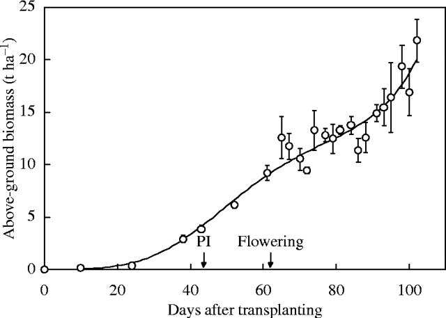
Annual crops often exhibit S-shaped growth patterns (Williams, 1964; Hunt, 1982) and the logistic equation has long been used to describe those patterns (Verhulst, 1838). However, as reported in this paper, in 1997, a curious growth pattern was observed for irrigated rice (Fig. 1). There was a slowing down in growth as the reproductive organs developed and a marked upswing in growth after flowering. Initially, simply for summarizing the data, a cubic polynomial was fitted to the natural logarithm of above-ground dry weight, to make variances more homogeneous (Hunt, 1982). The curve shown is back-transformed from the cubic polynomial. Although the curve describes the data adequately it is entirely empirical and the parameters have no biological meaning. In subsequent years somewhat similar patterns of growth were observed and this consistency prompted us to look for a more mechanistic description. It appears that the crop has two phases of logistic growth: the vegetative growth followed by the reproductive growth. At maturity, in high yielding rice, about half of the above-ground biomass is in the vegetative portion and half in the reproductive structures (Hay, 1995; Sheehy et al., 2000). Whether it would be useful to describe the growth pattern of rice as the consequence of two logistic curves, the first describing the vegetative and the second reproductive structures, is explored here.

Fig. 1.

Above-ground biomass (open circles) during growth of a rice crop, cultivar IR72, grown at IRRI in the dry season 1997. The curve (continuous line) shown is back-transformed from a cubic polynomial fitted to the natural logarithm of the data (r² = 0·98). The date of panicle initiation (PI) and the start of flowering are indicated.

METHODS

Experiments

The data on crop biomass and its components were obtained in various experiments on high yields and nitrogen uptake in transplanted, irrigated rice. Crops were grown at the International Rice Research Institute, Philippines, Los Baños (14°11′N, 121°15′E) in the dry season (January–May) using standard practices (Cassman et al., 1993; Maclean et al., 2002). The elite indica-type rice cultivar IR72 and breeding lines of the new plant type (NPT; Peng et al. 1994) were used. Full details are given in Sheehy et al. (2000, 2001, 2004a, b). A summary of the cultivars, transplanting dates, crop duration and yields is given in Table 1. Samples for above-ground biomass were taken at frequent intervals throughout crop duration. The biomass samples were separated into leaves, sheaths plus culm, dead matter, and panicles (the rice inflorescence) and oven dried before weighing. Panicle initiation was recorded in each experiment by dissecting sample plants to identify the day on which a reproductive meristem could first be distinguished on the stem apex.

Table 1.

Details of the irrigated rice crops

Cultivar	Year	Actual yield (t ha−1)	Predicted potential yield (t ha−1)	Transplanting date	Panicle initiation (DAT)	Crop Duration (days)	Remarks
IR72	1997	11·6 ± 0·7	11·4	27 Jan.	43	102	El Niño year (Sheehy et al., 2000)
	1998	11·6 ± 0·3	10·6	28 Dec.	39	101	Dry year (Sheehy et al., 2000)
	1999	8·1 ± 0·2	8·9	4 Jan.	38	105	Average year (Sheehy et al., 2001)
	2000	7·6 ± 0·1	9·1	10 Jan.	42	107	Unusually wet year (unpubl. data)
	2001	7·8 ± 0·1	8·8	5 Jan.	40	101	Average year (Sheehy et al., 2004b)
NPT
(IR65598-112-2)	1997	11·6 ± 0·5	11·4	27 Jan.	56	116	El Niño year (Sheehy et al., 2000)
(IR65564-44-5-1)	1998	12·0 ± 0·3	10·6	28 Dec.	46	108	Dry year (Sheehy et al., 2000)
(IR68011-15-1-1)	1999	7·0 ± 0·2	8·9	4 Jan.	53	114	Average year (Sheehy et al., 2001)

Yields are given at 14 % moisture content (86 % dry matter).

El Niño years in the Philippines are exceptionally sunny and dry.

Potential predicted yield is from the model given in Sheehy et al. (2004c).

Theory

The logistic growth model can be written as an equation for exponential growth with a feedback term that slows the rate of growth as the carrying capacity or upper limit is reached (Murray, 1993)

where W is the weight of the crop, t is time, g is a growth rate parameter and U is the upper limit of W as t → ∞. The logistic equation is the solution to eqn (1)

where W₀ is the initial weight of the crop.

Next the crop is divided into vegetative and reproductive structures and each of them is described using logistic equations. For vegetative growth W_v > 0 when t_m ≥ t ≥ 0, where the crop is transplanted when t = 0, and t_m is the age of the crop at maturity in days after transplanting. For the reproductive structures (panicles) W_p > 0 when t_m ≥ t ≥ t_pi, where t_pi is the age of the crop at panicle initiation. The growth rate of the crop at any time can be written as the sum of the growth rates of the two components

where the subscripts v and p refer to vegetative and panicle growth, respectively. The weight of the crop, W(t), is now described as the sum of two logistic curves

Data analysis

The logistic equations were fitted to the mean values of dry weights of the vegetative component (leaves, sheaths plus culm, dead matter) and the panicle (Table Curve 2D 4.0 for Windows, 1997 by SPSS Inc.; equation 8074 was used). The particular form of the logistic equation available was written as

where the parameter b is the point of inflection, i.e. when t = b, W = a/2 and dW/dt is a maximum (a/4c). The other two parameters are related to those in eqn (2) in the following way U ≡ a, g ≡ 1/c and W₀ = a/[1 + exp(b/c)]. The vegetative curves were fitted with t = DAT (days after transplanting) and the panicle curves were fitted with t = DAPI (days after panicle initiation). The two curves were then added together and plotted with the above-ground biomass. In rice, timing the final harvest at maturity is a matter of fine judgement to maximize yield, when most grains have finished filling and fewest have been shed. In 1997, the crops may have been harvested early, but predictions using a growth model suggest yield had reached a maximum (Table 1).

RESULTS

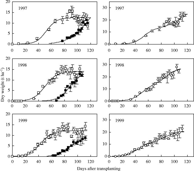
The data and fitted curves for the two cultivars are shown in Figs 2 and 3 (left panels). The curves were added together and are shown in the right panels; the data points are the total above-ground biomass. Values of the parameters together with the coefficients of determination (r²) are given in Table 2. It is clear that the logistic curves fitted the data well and the sum of the two curves described the data adequately. The combined logistics pass through the data, but a graph of the data alone would hardly have suggested an underlying bi-phasic structure. Furthermore, the overall pattern appeared to vary from year to year, whereas the two components were much more consistent in their shape (Figs 2 and 3). For IR72, panicle initiation was observed at about 40 DAT and the maximum growth rate of the vegetative component was predicted to be at about 43 DAT. Equivalent figures for the NPT were panicle initiation at 52 DAT and maximum vegetative growth at 47 DAT. The maximum growth rates of the vegetative component of IR72 and the NPT were about 0·35 t ha⁻¹ and 0·37 t ha⁻¹. The maximum growth rates of the panicle were on average 0·32 t ha⁻¹ at 42 DAPI for IR72, and 0·33 t ha⁻¹ at 45 DAPI for the NPT.

Fig. 2.

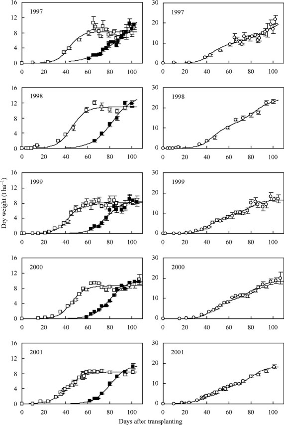
Above-ground biomass (open circles), and its components [vegetative parts (open squares) and panicle (solid squares)] for crops of IR72 grown in the dry season at IRRI between 1997 and 2001. The error bars are standard errors based on six replicates. Separate logistic curves fitted to the vegetative parts and to the panicles are shown in the graphs on the left. On the right, the line is the sum of the two logistic curves, shown with above-ground biomass; note that this line is not fitted to the data points shown.

Fig. 3.

As for Fig. 2, but crops of the new plant type (NPT) grown between 1997 and 1999.

Table 2.

The parameter values for the logistic curves (eqn 4: W = a/{1 + exp[−(t − b)/c]}) describing vegetative and reproductive growth together with the coefficient of determination (r²)

		Vegetative							Panicle
Cultivar	Year	a	b	c	r2	a	b	c	r2
R72	1997	8·3 (0·26)	43·0 (2·02)	5·7 (2·12)	0·90	15·7 (4·39)	50·4 (8·50)	14·5 (2·85)	0·96
	1998	10·9 (0·31)	45·3 (1·29)	6·5 (1·21)	0·98	13·9 (2·07)	43·4 (3·69)	9·2 (2·33)	0·98
	1999	8·2 (0·17)	42·5 (0·92)	6·1 (0·83)	0·97	8·5 (0·59)	38·9 (1·77)	7·1 (1·54)	0·93
	2000	8·6 (0·22)	45·4 (1·11)	5·9 (1·07)	0·96	10·2 (0·43)	38·3 (1·09)	7·8 (0·82)	0·98
	2001	8·4 (0·18)	41·3 (0·65)	7·4 (0·65)	0·98	10·2 (0·47)	40·5 (1·12)	7·3 (0·71)	0·99
NPT
(IR65598-112-2)	1997	12·5 (0·50)	52·3 (4·02)	7·9 (3·30)	0·88	21·1 (12·34)	58·5 (16·51)	14·6 (4·35)	0·97
(IR65564-44-5-1)	1998	14·1 (0·44)	50·3 (1·76)	9·1 (1·46)	0·97	13·8 (1·71)	42·6 (3·01)	9·0 (1·81)	0·96
(IR68011-15-1-1)	1999	12·2 (0·38)	43·3 (1·80)	9·0 (1·51)	0·94	9·1 (0·53)	35·2 (1·63)	9·5 (1·06)	0·98

The numbers in parentheses are standard errors, the units of a are t ha⁻¹, the units of b and c are days.

There was a highly significant correlation (P < 0·001) between the observed grain yields and the predicted yield potentials using the model of Sheehy et al. (2004c) with a radiation use efficiency of 2·6 g above-ground dry weight per MJ intercepted photosynthetically active radiation. The asymptotic value for the panicle was significantly correlated (P < 0·001) with the predicted yield potential. There was no correlation for the asymptotic value for vegetative growth with observed or predicted yields.

There are some interesting features that emerge from the bi-phasic approach to partitioning growth and to illustrate them we have used the mean values of the parameters for IR72 to construct the growth rate curves (Fig. 4A) for the vegetative and reproductive components. It can be seen in Fig. 4A that the panicle, whose growth is largely heterotrophic, has a maximum growth rate about the same as that achieved by the autotrophic vegetative component. The panicle commences growing rapidly a few days after the maximum growth rate of the vegetative components was realized and marks the beginning of a decline in the rate of vegetative growth. The maximum growth rate of the panicle occurs when growth in the vegetative components has ceased. Furthermore, it took about the same time for the panicle to attain its maximum growth rate as it took the vegetative component. The two curves (Fig. 4A) demonstrate a high degree of coordination between the two phases of growth. The vegetative and reproductive components of growth have been added together to produce a cumulative growth curve for IR72 (Fig. 4B). The distinctive pattern of growth of the crop can be seen clearly.

Fig. 4.

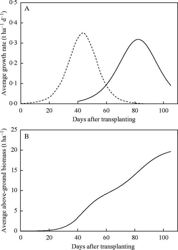
(A) Rates of growth for the vegetative parts (broken line) and the panicle (continuous line) during growth of a rice crop. The parameter values in Table 2 were averaged for IR72 across all years to produce composite logistic curves for vegetative parts and panicle; these were differentiated to produce the curves of growth rate. (B) The cumulative pattern of above-ground growth (solid line) of the cultivar IR72 generated by adding the composite logistic descriptions of vegetative and reproductive growth.

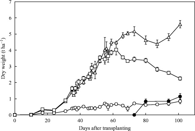
It was noteworthy that in every case (Figs 2 and 3) there was a dip in the weights of the vegetative components towards maturity, which the logistic curve cannot follow. To explain this it is shown how the individual vegetative parts (leaves, sheaths plus culm, dead matter and roots) varied during growth in a typical year, 2001 (Fig. 5). It is evident that there was a decline in the weight of leaves from about 60 DAT onwards and the weight of the sheaths plus culm also declined, but then recovered weight during the final 10 d. Rice is a weak perennial and a new generation of tillers starts to grow just before maturity; this ability is exploited in ratoon crops (IRRI, 1988). As expected, dead matter increased towards maturity but there appeared to be no loss of root weight during this period.

Fig. 5.

Vegetative biomass during growth of a rice crop, IR72 in 2001, plotted separately for leaves (open squares), sheaths plus culm (open triangles), roots (open circles) and dead matter (filled circles).

DISCUSSION

In these experiments, harvests were often taken at short intervals (2–3 d) to follow changes in components of biomass, tillering and grain development in detail, particularly as the crop moved from vegetative to reproductive growth. The more standard procedure is to take harvests at intervals of 7–10 d, in which case the bi-phasic growth pattern may not be observed. The determinate growth of monocarpic plants has often been adequately described by simple curves such as polynomials or the logistic curve (Hunt, 1982; Yin et al., 2003). Nevertheless, once the logistic growth pattern of the two components is in mind, it can be seen in other sets of data for rice (e.g. ‘Kindinga’, Enyi, 1962; IR72, N2 treatment, Dingkuhn et al., 1992). As far as is known, this bi-phasic growth pattern has not been reported in other cereals. It could occur wherever reproductive growth lags behind the growth of vegetative parts, and should be evident in experimental data when the harvests are sufficiently frequent.

Not surprisingly, there was a strong correlation between predicted yield potentials and the asymptotic values for the panicles, indicating that the change in weather from year to year influences final panicle weight. However, the lack of a correlation for the vegetative growth component suggests that its maximum weight is influenced to a lesser extent. Clearly, it is the weather during panicle growth that has the strongest influence on grain yield.

Meyer (1994) proposed a bi-logistic curve for modelling growth when there are two distinct phases, each with a logistic pattern. The model, with six parameters, is simply two logistic curves added together and can be fitted to data by a non-linear least-squares procedure. A variety of curves can be produced with the bi-logistic model, depending on the relative timing of the two logistic components, and on the relative size of the exponential growth terms. The curves were often sigmoid, but not necessarily symmetrical, so that the underlying logistic structure was not always evident on inspection. Indeed, when one looks at the data reported here for above-ground biomass, there is no obvious simple pattern that would describe each year. The combined logistics curve described here passes through the data, but the data do not obviously suggest that there is an underlying bi-phasic structure. Meyer (1994) pointed out that the bi-logistic is especially useful because the parameters are capable of interpretation in terms relevant to the system being modelled.

A possible application of the bi-logistic approach would be to retrieve the logistic curve of the panicle from the overall curve for above-ground biomass. Measurements of biomass as a whole can be made with less effort than separating the component parts, and if made by remote sensing they could also be obtained at frequent intervals (Inoue et al., 2002; Hansen and Schjoerring, 2003). Fitting a bi-logistic curve and deconvolving to obtain a logistic curve for panicle growth, the second component, would allow direct estimation of the weight of the harvested part of the crop. The alternative would be to multiply biomass by the harvest index. But harvest index can vary from year to year, and with cultivar, so a procedure that did not rely on providing an estimated figure for harvest index would be of great value.

Understanding how rice grows is important. In Asia, where rice is the principal cereal, the population will rise by an estimated 1·6 billion (UNFPA, 1999) during the next 50 years. Increases in rice productivity (per unit area, per unit of water, per unit of labour) are essential to lower the price of rice for the benefit of poor rice consumers (Dawe, 2000). Recognizing the significance of the two fundamental components of crop biomass in shaping the overall pattern of rice growth should be of great benefit to crop physiologists and modellers.

LITERATURE CITED

- Cassman KG, Kropff MJ, Gaunt J, Peng S. 1993. Nitrogen use efficiency of rice reconsidered: what are the key constraints? Plant and Soil 155/156: 359–362. [Google Scholar]
- Dawe D. 2000. The contribution of rice research to poverty alleviation. In: Sheehy JE, Mitchell PL, Hardy B, eds. Redesigning rice photosynthesis to increase yield. Amsterdam, The Netherlands: Elsevier. [Google Scholar]
- Dingkuhn M, De Datta SK, Javellana C, Pamplona R, Schnier HF. 1992. Effect of late-season N fertilization on photosynthesis and yield of transplanted and direct-seeded tropical flooded rice. I. Growth dynamics. Field Crops Research 28: 223–234. [Google Scholar]
- Enyi BAC. 1962. Comparative growth rates of upland and swamp rice varieties. Annals of Botany 26: 467–487. [Google Scholar]
- Hansen PM, Schjoerring JK. 2003. Reflectance measurement of canopy biomass and nitrogen status in wheat crops using normalized difference vegetation indices and partial least squares regression. Remote Sensing of Environment 86: 542–553. [Google Scholar]
- Hay RKM. 1995. Harvest index: a review of its use in plant breeding and crop physiology. Annals of Applied Biology 126: 197–216. [Google Scholar]
- Hunt R. 1982.Plant growth curves. London: Edward Arnold Publishers. [Google Scholar]
- Inoue Y, Kurosu T, Maeno H, Uratsuka S, Kozu T, Dabrowska-Zielinska K, Qi J. 2002. Season-long daily measurements of multifrequency (Ka, Ku, X, C, and L) and full-polarization backscatter signatures over paddy rice field and their relationship with biological variables. Remote Sensing of Environment 81: 194–204. [Google Scholar]
- IRRI. 1988.Rice ratooning. Los Baños, Philippines: International Rice Research Institute. [Google Scholar]
- Maclean JL, Dawe DC, Hardy B, Hettel GP. 2002.Rice almanac, 3rd edn. Manila, Philippines: International Rice Research Institute. [Google Scholar]
- Meyer P. 1994. Bi-logistic growth. Technological Forecasting and Social Change 47: 89–102. [Google Scholar]
- Murray JD. 1993.Mathematical biology. Berlin: Springer-Verlag Publishers. [Google Scholar]
- Peng S, Khush GS, Cassman KG. 1994. Evolution of the new plant idiotype for increased yield potential. In: Cassman KG, ed. Breaking the yield barrier. Proceedings of a Workshop on Rice Yield Potential in Favorable Environments. International Rice Research Institute, Manila, Philippines, December 1993, 5–20. [Google Scholar]
- Sheehy JE, Dionora MJA, Mitchell PL. 2001. Spikelet numbers, sink size and potential yield in rice. Field Crops Research 71: 77–78. [Google Scholar]
- Sheehy JE, Mitchell PL, Dionora MJA, Tadashi T, Peng SB, Khush GS. 2000. Unlocking the yield barrier in rice through a nitrogen-led improvement in the radiation conversion factor. Plant Production Science 3: 372–374. [Google Scholar]
- Sheehy JE, Mnzava M, Cassman KG, Mitchell PL, Pablico P, Robles RP, Ferrer AB. 2004. Uptake of nitrogen by rice studied with a 15N point-placement technique. Plant and Soil 259: 259–265. [Google Scholar]
- Sheehy JE, Mnzava M, Cassman KG, Mitchell PL, Pablico P, Robles RP, Samonte HP, Lales JS, Ferrer AB. 2004. Temporal origin of nitrogen in the grain of irrigated rice in the dry season: the outcome of uptake, cycling, senescence and competition studied using a 15N-point placement technique. Field Crops Research 89: 337–348. [Google Scholar]
- Sheehy JE, Peng S, Dobermann A, Mitchell PL, Ferrer A, Yang J, Zoue Y, Zhong X, Huange J. 2004. Fantastic yields in the system of rice intensification: fact or fallacy? Field Crops Research 88: 1–8. [Google Scholar]
- SPSS Inc. 1997. Table curve 2D 4.0 for Windows, User's Manual, Now at Systat Software, Inc., Richmond, California, USA. http://www.systat.com [Google Scholar]
- UNFPA. 1999. The State of World Population 1999. United Nations Population Fund, New York, USA. http://www.unfpa.org/upload/lib_pub_file/49_filename-swp99.pdf [Google Scholar]
- Verhulst PF. 1838. A note on population growth. Correspondence Mathematiques et Physiques 10: 113–121 [in French] [cited by Murray, 1993]. [Google Scholar]
- Williams RF. 1964. The quantitative description of growth. In: Barnard C, ed. Grasses and grasslands. London: MacMillan, 89–101. [Google Scholar]
- Yin X, Goudriaan J, Lantinga EA, Vos J, Spiertz HJ. 2003. A flexible sigmoid function of determinate growth. Annals of Botany 91: 361–371. [DOI] [PMC free article] [PubMed] [Google Scholar]