Abstract
• Background and Aims Physiological and architectural plant models have originally been developed for different purposes and therefore have little in common, thus making combined applications difficult. There is, however, an increasing demand for crop models that simulate the genetic and resource‐dependent variability of plant geometry and architecture, because man is increasingly able to transform plant production systems through combined genetic and environmental engineering.
• Model GREENLAB is presented, a mathematical plant model that simulates interactions between plant structure and function. Dual‐scale automaton is used to simulate plant organogenesis from germination to maturity on the basis of organogenetic growth cycles that have constant thermal time. Plant fresh biomass production is computed from transpiration, assuming transpiration efficiency to be constant and atmospheric demand to be the driving force, under non‐limiting water supply. The fresh biomass is then distributed among expanding organs according to their relative demand. Demand for organ growth is estimated from allometric relationships (e.g. leaf surface to weight ratios) and kinetics of potential growth rate for each organ type. These are obtained through parameter optimization against empirical, morphological data sets by running the model in inverted mode. Potential growth rates are then used as estimates of relative sink strength in the model. These and other ‘hidden’ plant parameters are calibrated using the non‐linear, least‐square method.
• Key Results and Conclusions The model reproduced accurately the dynamics of plant growth, architecture and geometry of various annual and woody plants, enabling 3D visualization. It was also able to simulate the variability of leaf size on the plant and compensatory growth following pruning, as a result of internal competition for resources. The potential of the model’s underlying concepts to predict the plant’s phenotypic plasticity is discussed.
Key words: Plant architecture, phenotypic plasticity, demand functions, competition among sinks, source–sink relationships, structural‐functional models
INTRODUCTION
Physiological crop models are commonly used to answer agronomic questions (e.g. Jones et al., 1998; Brisson et al., 2002). They typically describe the flux of external resources through the apparatus ‘plant’ into a pool called yield. The plant is thereby seen as a set of invariable (genetic) rules and parameters that govern resource acquisition and conversion on a field area basis, organized by a phenological timetable. This approach is particularly robust for field crops forming homogenous canopies, whose behaviour is quite insensitive to aggregation of morphological entities into larger compartments (e.g. big‐leaf concept as in Allen et al., 1998 or Jones and Kiniry, 1986). The same cannot be said for heterogenous or widely spaced populations, or culture systems in which plant architecture and geometry are of specific interest to the producer. In fact, modern plant production systems are increasingly shaped by genetic, agronomic and environmental engineering, which seek specific structural features of the crop (Prakash, 2001; McFerson and Pierce, 2003). The development and management of such systems require models that provide plant architectural detail, in addition to resource flow and yield. Moreover, and most challenging, these models should be able to simulate, depending on the application, some of the plant’s phenotypic plasticity that results from genetically controlled feedbacks among growth (biomass acquisition), differentiation (phenology, morphogenesis) and the physiological condition of the organism (e.g. stresses).
The first plant architectural models were built from mathematical algorithms because of the needs of computer graphics and were entirely descriptive. In contrast to crop models that describe resource budgets and flows, architectural models describe structure based on topological principles (descendance of organs, e.g. sympodial or monopodial structure) and plant geometry (organ shape and size, phyllotaxy). Modelling concepts and software for constructing 3D plants date back to the invention of L‐systems (Lindenmayer, 1968) and fractals or graftals (Smith, 1984), which allow the assembling of complex structures (Prusinkiewicz et al., 1988). Evolved software such AMAP (de Reffye et al., 1988), ONYX‐TREE (www.OnyxTREE.com, 2003) and X‐FROG (www.greenworks.de, 2001; www.xfrog.com, 2003) are commonly used in townscaping, landscaping, advertising and computer graphic games, but so far have found few uses in agro‐ecological research.
The first 3D plant models used in biological research were static and either descriptive (derived from plant digitalization) or synthetic. They served, for example, to compute light interception and distribution (Dauzat, 1994; Dauzat and Eroy, 1997; Chelle and Andrieu, 1998) but did not consider biological processes. Recently, structural‐functional plant models have been developed that perform dynamic simulations of plant morphogenesis, such as LIGNUM (Perttunen et al., 1996; Sievanen et al., 2000), Cotons (Jallas et al., 2000) derived from the physiological model Gossym (Baker et al., 1983), AmapHydro (de Reffye et al., 1999) and GroGra (Kurth and Sloboda, 1997). In these models, a phenological engine responsible for organogenesis provides for the compartments among which the incrementally acquired biomass is distributed. In AmapHydro and Cotons, a notion of resource‐dependent phenotypic plasticity is realised in different ways, either through a hydraulic architecture that is sensitive of differential transpiration among plant parts (AmapHydro) or through sink modulation as a function of internal competition for resources (Cotons/GOSSYM).
Generally, these structural‐functional models are discrete‐event simulators of high complexity, and not mathematical models in the strict sense. Some problems arise from this, namely (1) high computational time requirements, particularly for complex plants such as trees; (2) difficult calibration of a large number of parameters, frequently by optimization when they cannot be measured directly; and (3) opaqueness of the simulation process from a mathematical point of view. As a result, bug‐proofing is difficult, and it is quite possible to achieve perfect fit with a flawed model if powerful optimization techniques such as genetic algorithms are applied to a large number of parameters. This problem is bound to be aggravated in models that simulate plastic behaviour resulting from multiple internal feedbacks, as opposed to classic crop models where biomass partitioning among organs is forced by rigid phenological or allometric rules that can be calibrated directly. For example, Dusserre et al. (2002) demonstrated for cotton that many processes affecting sink strength at the plant scale, such as organ appearance rate, abortion probability and potential size, depend on competition relationships within the plant.
This study presents a new structural‐functional model that seeks to overcome some of these limitations by choosing a mathematical approach and a highly simplified physiological basis. GREENLAB is derived from the architectural models AMAPsim (http://amap.cirad.fr/ amapsim), an automaton‐based simulator of organogenesis, and AMAPhydro (de Reffye et al., 1999), which introduces a hydraulic architecture. Biomass acquisition is thereby derived from transpiration by assuming water use efficiency (WUE) to be constant (Howell and Musick, 1984; Stanhill, 1986), and emphasis is on topological structure that determines the dynamics of sinks. Both AMAP models are prone to the problems mentioned above, particularly computation time requirements. In GREENLAB we sought to avoid these problems by extracting the hidden equations situated inside a simulation process that approximates the genesis of an observed plant. The use of a small number of parameters and rules in a single mathematical construction enabled speedier execution and greater mathematical transparency, but on the other hand prohibited any arbitrary or discrete forcing as is commonly found necessary in biological models. This paper introduces GREENLAB’s principal features, demonstrates its potential to represent (or recreate) complex morphogenetic sequences, and evaluates its theoretical potential (or limitation) to simulate phenotypic plasticity by extrapolation.
THE MODEL
Underlying concepts
The GREENLAB model was designed to provide dynamic representations of the morphogenesis and architecture of a plant on the basis of a minimal number of mathematical equations and metamorphic rules. The model is parameterized by optimization procedures using a fairly extensive set of botanical and morphological descriptors measured on a sample plant in the course of its development, and subsequently is able to construct identical or divergent phenotypes by implementing the same rules and parameters for the same or different environments. It is thereby capable of simulating some of the phenotypic plasticity of a genotype, as far as these architectural and morphological deformations result from fluctuations in biomass acquisition. The model, however, does not claim to be fully mechanistic with regards to physiological processes and fluxes involved in plant growth. In fact, it is empirical and some of its underlying rules, such as a non‐linear relationship between leaf surface and assimilation rate, are rather intuitive. The model was developed to explore the potential to mimic with a small set of mathematical rules not only a complex plant architecture but also its morphogenesis and resource‐dependent variability.
The model functions parameterized by optimization are (1) a hypothetical, non‐linear relationship between leaf size and assimilation, and (2) functions describing the general shape of sink‐strength kinetics for each type of organ from its initiation to maturity. Model parameters pertaining to botanical structure and metamorphic and allometric rules, essentially non‐mathematical, are set manually before optimization. The types of parameters used in the model are listed in Table 1.
Table 1.
Key parameters used in GREENLAB
| Topological parameters |
| Physiological age (PA) of an organ and number PAs present in the structure |
| Number of microstates for a given macrostate (Phytomers/growth unit) |
| Number of macrostates (growth units) for a given bearing axis |
| Occupancy and transition law between the states (Markov Matrix) |
| Functioning parameters |
| Base temperature (set to 5° C for sunflower) |
| Number and thermal duration of growth cycles |
| Thermal duration of organ expansion tO |
| Empirical parameters r1, r2 relating leaf transpiration to leaf size |
| Water use efficiency (biomass per water transpired) |
| Sink parameters of the beta law function pO(i): a, b |
| State variables |
| Number of organs of PA: O at CA: T: NTO (computed using automaton algorithms) |
| Sizes of the organs of PA: O and CA i in the plant n GC aged: qOi,n |
| Geometric and allometric parameters |
| Insertion angles of organs |
| Specific leaf area (surface per fresh weight) |
| Organ water content |
| Allometric parameters (dimensional and weight relationships among organs, e.g. leaf petiole and blade) |
Biological assumptions
Modelling of plant growth and architecture relies on biological assumptions borrowed from botany and crop physiology. We distinguish between trophic (growth related) and phenological (development and differentiation related) processes. At the present stage of model development, at which we aim at evaluating the principal concepts, these assumptions are cast in a small number of basic rules.
Phenological processes.
We consider here two aspects of phenology, the temporal and topological organization. The temporal organization is based on thermal time by accumulating the daily mean air temperature above a genetic‐based temperature (Gao et al., 1992). No optimal or maximal temperatures (Dingkuhn and Miezan, 1995) are considered at this stage in order to keep the model simple. During each period, or growth cycle (GC), a cohort of organs is produced. For simplicity we assume the thermal time elapsing during a GC to be constant throughout plant development. Maximal organ life‐spans are also set in thermal time. A GC may measure between a few days (in the case of herbacious plants) and 1 year (temperate trees). The GC also serves as a generalized time increment for model execution, which therefore depends on the species and is quite different from that of common crop models (typically, 1‐d time increments). The set of phytomers produced during one GC is called the growth unit (GU). The same GC is used to control organ production, biomass fabrication and biomass partitioning, in order to link the phenomena by a set of equations that generate feedback. Organ expansion and useful life‐span may cover several GCs and may continue even after organogenesis has stopped due to floral initiation in annual plants.
The topological organization is based on discrete botanical entities (organs) of different types, such as internodes, leaves, flowers and their components, which generally represent metamorphic variations of the basic unit, i.e. the phytomer. Each phytomer is produced by terminal or axillary meristems, resulting in a tree structure. The organs themselves evolve on their individual, finite, thermal‐time axes and are therefore characterized by physiological age (PA), which is an important determinant of their growth and branching behaviour.
A phytomer consists of an internode and a terminal node bearing leaves (or their various metamorphoses, for example in the case of reproductive organs) and axillary buds containing a fresh meristem. The parameters characterizing a specific phytomer depend on the type of meristem it originated from. Meristem properties depend on the general type (shoot or root, apical or axillary) and position within the plant structure (e.g. ortho‐ or plagiotropic behaviour). In contrast to apical meristems, which extend existing axes (e.g. branches, tillers, stems), axillary buds create new axes (branching).
Development processes can be restricted to a given organ and will then be governed by its PA. Plant‐level development processes such as floral induction, however, are systemic and affect many or all shoot meristems, depending on dominance rules. These systemic phenomena require the notion of a chronological age (CA) for the entire plant, even in the case of indeterminate or perennial plants.
Biomass growth.
For the current, rather conceptual, studies with GREENLAB, we assume dry matter (DM) assimilation to be proportional to transpiration, i.e. water use efficiency (WUE) to be constant (Howell and Musick, 1984). For example, WUE of the C4 crop maize is about 4 mg DM g–1 H2O, and that of the C3 crop potato is about 2 mg DM g–1 H2O if measured over longer periods (Stanhill, 1986). WUE is not much affected by crop water deficit but depends on climate, particularly evaporative demand (Hsiao and Xu, 2000). For the purpose of obtaining a notion of volume and weight of the wet plant biomass, we assume an arbitrary moisture content of 0·8 (water divided by total weight).
In its conceptual, extremely simple version presented here the model applies an evaporative demand (Allen et al., 1998) homogeneously to all leaf surfaces, and translates it into a proportional transpiration rate. Two leaf‐size‐dependent, empirical attenuation parameters derived from the optimization during model parameterization calibrate the relationship between evaporative demand and leaf transpiration, and thus biomass assimilation. Into this summary equation are lumped a number of physiological processes such as differential exposure of leaves (shading) and regulation of stomatal resistance, which at this point are not considered in detail. (Two more detailed model versions are being developed, one that simulates in detail the 3D light distribution in the canopy as a means for weighted implementation of evaporative demand, and another that implements a full carbon and water balance at the plant scale. Only this latter version will simulate a root system and the effects of water deficit.)
The amount of fresh biomass produced during a GC, considered a transitory reserve pool, is entirely converted into new organs that have been initiated according to the automaton‐driven phenology model. It is assumed that organs of a given type do not vary in shape nor in the duration and kinetics of the relative sink strength they exert during their growth. However, they may attain variable final sizes, depending on how many sinks have to share the transitory reserve pool. Because organ growth periods may be considerably longer than a GC, growing organs of the same type but of different ages may coexist and exert different sink strength on a common pool of assimilates. No feedback of biomass acquisition on organogenesis is simulated in the current model, but this is being developed for a future model version.
Modelling
Modelling of organogenesis using dual‐scale automaton.
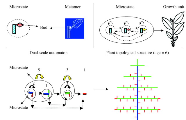
GREENLAB uses automaton theory (Yan et al., 2002), whereby the microstate, macrostate and the jump relationships among them are employed to represent phytomers, GUs and the metamorphic rules, respectively. In order to simulate evolving botanical structures, programmers use stochastic automatons which are the basic units of an informatic grammar. The advantages of Markovian automatons are that they operate in cycles and have versatile rules of state transition and of occupancy. These automatons are also easy to calibrate with experimental data because their mathematical behaviour is well studied. The analogy of Markovian automatons with buds in a botanical structure, however, is intuitive: the different states of the automaton correspond to physiological age classes, and the transitions of the automaton correspond to the bud’s differentiation, or to its generation of an axillary bud (automaton).
The GU produced in a given GC is a cohort of new phytomers and called a macrostate, and each phytomer is a microstate. The macrostate can be implemented repeatedly until the law of occupancy for the given physiological age is fulfilled, resulting in a bearing axis (BA). The completed BA can either terminate its development, or its terminal bud is transformed to assume a different physiological age according to the automaton transition law. Thus a non‐terminal macrostate produces microstates of different physiological age, called axillary branches. New phytomers can only bear leaves, and at least one further GC is required for them to produce fruits or branches. The series of macrostates and microstates correspond to semi‐Markov chains that can deterministically or stochastically generate plant structures.
Figure 1 shows an automaton and the resulting plant structure resulting from the step‐by‐step implementation of organogenesis. The dual‐scale reference automaton used here is thus able to construct complex plant architectures while being more flexible than the reference axis automaton used in previous models such as AMAPsim (http://amap.cirad.fr/amapsim).
Fig. 1. Simulation with automata of a plant with three physiological age levels (PA) and ten chronological ages (CA). The automaton plot is shown on the left and the botanical observation on the right in each case.
The organogenetic process provides the type, status and number of different organs that are present in the plant structure during a given GC, and thus allows simulation of biomass allocation among these organs according to their current, relative demands. The root system is at present not considered, but efforts are under way to do so.
Modelling of biomass acquisition.
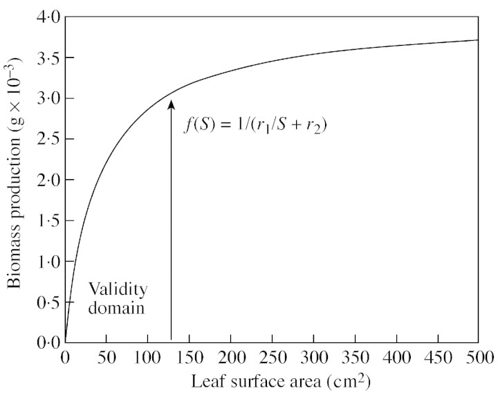
We suppose that the biomass produced by each leaf depends only on its surface area, S, according to an empirical, non‐linear function f(S, r1, r2), where r1 and r2 are parameters to be computed by optimization methods (Zhan et al., 2002). The following equation is used to approximate observations:

This function is a hyperbola in the valid domain for plant growth (Fig. 2). Note that the biomass production of each leaf becomes proportional to leaf surface if parameter r2 is zero. The biomass Qn generated by all green leaves present at CAn can be expressed as follows:
Fig. 2. The empirical function of leaf biomass production in relation to individual leaf surface area, with the ‘hidden’ parameters r1 and r2 that are optimized during model calibration.

where NLk is the number of green leaves produced in the plant structure at CAk, each leaf having the corresponding surface area Sk.
The leaf‐size‐dependent function of assimilation is not based on physiological theory but permits, through parameter optimisation, to empirically lump much of the unknown effects of leaf age, mutual shading, nitrogen distribution within the canopy, and more, in one simple expression. It can be expected that in future model versions that will step‐wise include more physiological and environmental detail, this function will become increasingly linear and might at some point become obsolete. Empirical parameters so far obtained for the hyperbola generally lead to the shape presented in Fig. 2, indicating that smaller leaves have higher assimilation rates per unit area than larger ones.
Modelling of biomass distribution.
Biomass is allocated to organs according to their relative demand, and their volumes are calculated from their fresh weights. Empirical, allometric rules are used to determine the dimensions and shapes of organs from their volumes. We suppose that plant biomass available for distribution, Qn, during a period, GCn, is equal to the sum of all leaf contributions plus the reserves mobilized from the seed during the first cycle. (Redistribution of biomass within the plant is at this stage not considered in the model.)
We consider green (non‐senescent) organs, O (O = B, P, I, C, F; corresponding to leaf blade, peduncle, internode, secondary growth rings on the stem, and fruits or flowers), in the plant structure; pO (i) is the reference sink value. Qn – 1 is the biomass supply provided by the leaves for distribution among sinks present in the plant architecture that constitute the overall demand, Dn. For a plant structure at CAn, the biomass increment of organ O appearing at CAi on this structure is described as:

Consequently, biomass allocated to an organ is proportional to its demand and to the incremental pool of biomass for distribution, divided by the total plant demand (Marcelis et al., 1998).
The sink pO(i) depends on the organ PA, O, on growing organ period, tO, and on its expansion, GC i. To normalize the sink function p we set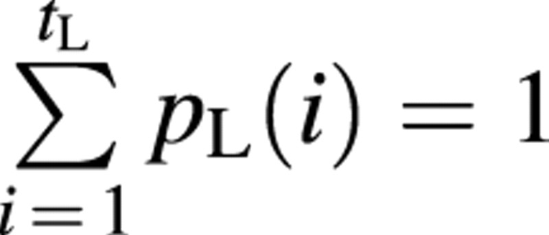 for the leaves. All other sink functions are normalized accordingly, resulting in
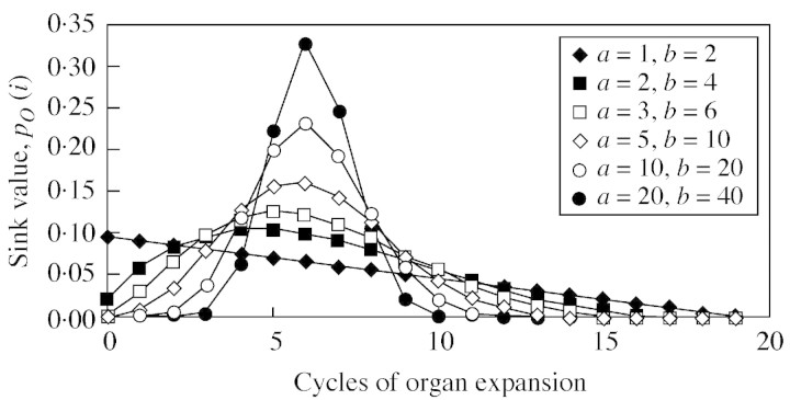
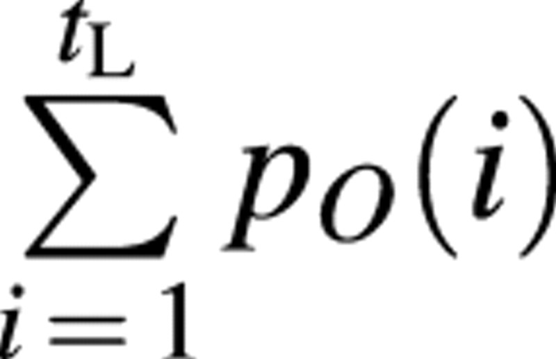 . The function type for pO(i) can be chosen by the user and should be able to fit typical biological kinetics such as bell or sigmoid shapes. The model uses a beta‐function by default:

Here, i assumes only integer values, while a and b are real numbers that can be computed by heuristic methods when fitting the plant architecture by using the generalized least‐square method (Zhan, 2002). Figure 3 shows different shapes of pO(i) depending on the values of parameters a and b, which indeed differ among organ types and plant species. The duration of growth tO of organ O can be forced from measurements.
Fig. 3. Different kinetics of organ demand for biomass pO(i) depending on the values of parameters a and b for a beta law (refer to eqn 5 in text).
Dn is the bulk demand of all growing organs during period tO (a fraction period of growth cycle GCn), described by eqn (5):

The total biomass qOi,n preserved in this organ is the sum of ΔqOi,n from GCi to GCn, i.e.:
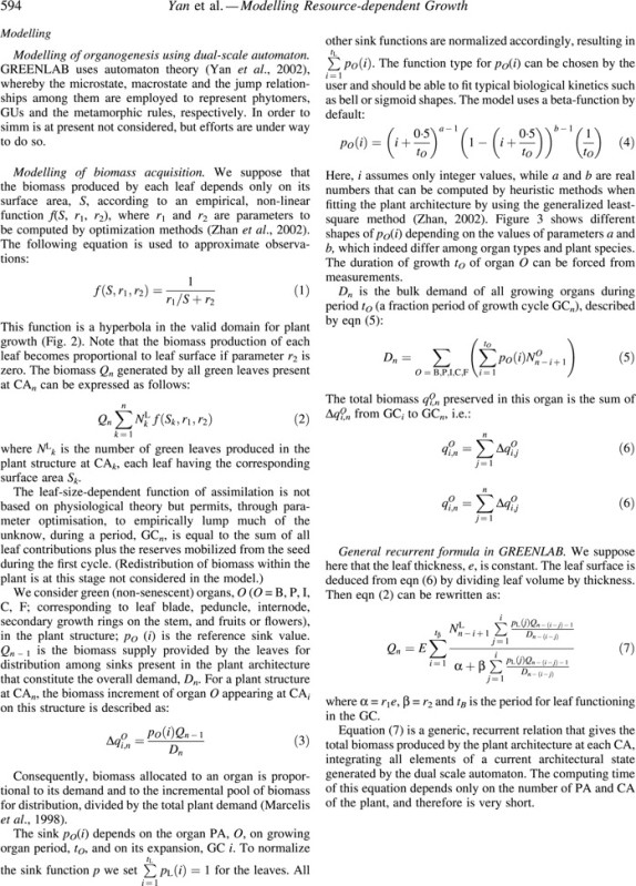
General recurrent formula in GREENLAB.
We suppose here that the leaf thickness, e, is constant. The leaf surface is deduced from eqn (6) by dividing leaf volume by thickness. Then eqn (2) can be rewritten as:
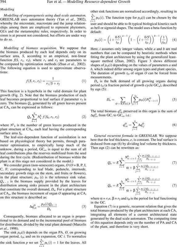
where α = r1e, β = r2 and tB is the period for leaf functioning in the GC.
Equation (7) is a generic, recurrent relation that gives the total biomass produced by the plant architecture at each CA, integrating all elements of a current architectural state generated by the dual scale automaton. The computing time of this equation depends only on the number of PA and CA of the plant, and therefore is very short.
SOME FEATURES OF GREENLAB
Construction of complex, virtual plant architectures using substructures
The model can simulate complex tree architecture with a high efficiency because it uses special algorithms using the decomposition of the tree in a stack of substructures identified by CA and PA (Yan et al., 2002). Each substructure having a given PA and CA is computed only once but can be represented repeatedly in a given tree architecture. In common software for tree simulation, computing time is proportional to the number of metamers, whereas that of the substructure method is proportional to the number of CA multiplied by the number of PA, enabling a 1000‐fold faster computation of a complex tree architecture than with classical bud‐by‐bud parallel simulation. This also permits visualisation of substructures of a given CA and PA.
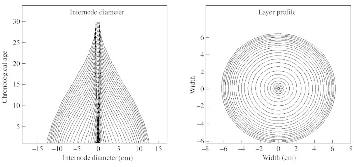
Simple rules are used to compute organ dimensions from their volume, which is in turn derived from their fresh weight. For example, leaf surface is computed from specific leaf area (SLA, surface per biomass), and leaf peduncles are assumed to be shaped as cylinders. Internodes consist of a central pith, (its size being set by the first internode expansion from the bud) and a stack of layers (rings) that correspond to secondary growth (Fig. 4). Lastly, the properties of fruits are approximated using appropriate geometric forms such as spheres.
Fig. 4. Vertical section (A) and cross‐section (B) of a simulated stem; pith (in the middle) and radial growth. The chronological age corresponds to the number of the Growth Unit.
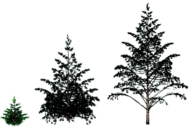
The monopodial Rauh (orthotropic branches) and Massart (plagiotropic) architectures found in pine, spruce, poplar and cherry were used to demonstrate the construction of trees using substructures (Figs 5 and 6). Buds have rhythmic activity and undergo programmed termination according to the PA automaton rules. The bearing axis of such a model is a replication of the same macrostate for a given PA. Its apical bud can generate a terminal branch by metamorphosis, involving a change in PA, after several repetitions of the same macrostate. The microstates in a macrostate can also be replicated several times and can bear lateral branches, whose PA is greater than that of their bearing axis. (Note that physiological age is not necessarily related to absolute age!) The PA of the lateral branches increases from top to bottom. In Fig. 5, an additional rule was introduced to simulate acrotony, the production of longer axes towards the distal end of a branch. Complex tree architectures can usually be simulated with very few levels of PA, such as six or less. Figure 5 shows a complex Rauh model with five levels of PA and a large number of substructures, resulting from step‐by‐step simulation of organogenesis, biomass acquisition and allocation, and organ shape and geometry. Figure 6 shows a tree simulated at 10, 20 and 30 years. The years in this case correspond to GCs. Features such as bending (resulting from branch weight, branching angle and branch thickness) are integrated in the simulation. The growth in length is exponential at the beginning and then becomes linear due to competition among sinks.
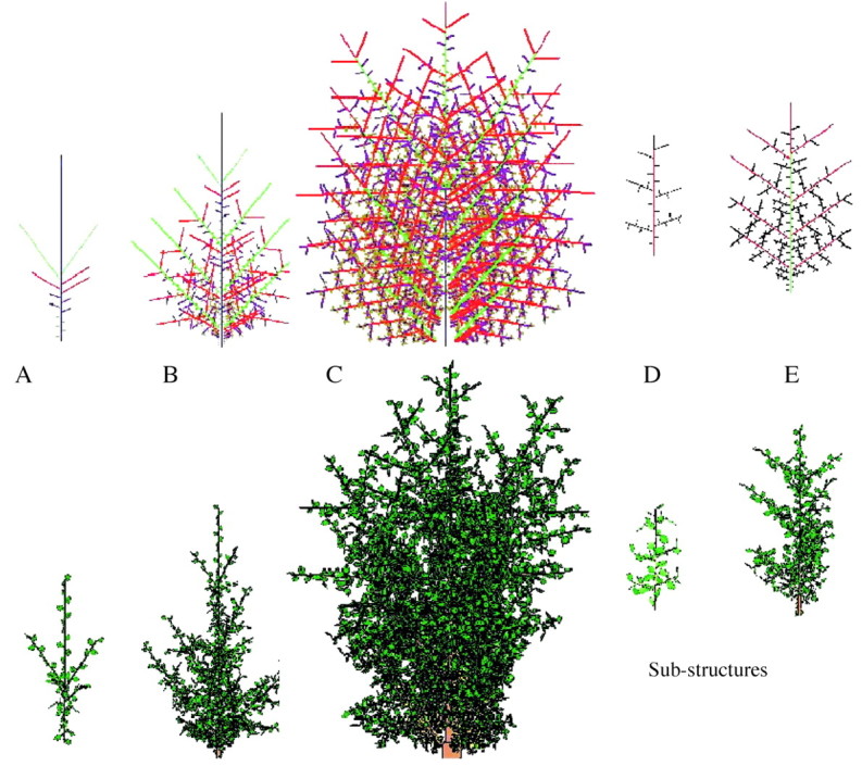
Fig. 5. A complex tree with Rauh architecture, simulated with five physiological age levels (PA) after completeion of (A) two, (B) five, and (C) ten growth cycles (GC), with sub‐structures of (D) PA = 2 at GC = 6, and (E) PA = 3 at GC = 4 (scales vary). Representation of the topological structure with differently coloured PA levels (top) and the corresponding 3D geometric structure carrying leaves (bottom).
Fig. 6. Simulated growth of a Massart model at three stages (10, 20 and 30 years), with branches bending according to their weight and geometry.
Fitting the model to real plants: an example
A field experiment on sunflower was conducted at the China Agricultural University in 2000, in order to establish a reference data file for calibration of the model (Guo et al., 2003). A large distance between plants (0·6 m) was chosen to minimize competition. Irrigation and nutrients were applied at non‐limiting rates. Weather data were collected at a nearby station and potential evapotranspiration was computed according to FAO guidelines.
Destructive measurements were conducted on two plants every 2 weeks. The fresh weight of each internode, petiole and blade, the diameter and length of each internode and petiole, and the leaf area of each blade were measured. The fresh weight of the inflorescence was also measured when it appeared. From these observations, allometric relationships were determined that describe, for example, specific weights of organs, specific leaf area (SLA), organ shape, or petiole versus leaf allometries.
Some model parameters, such as those describing relative sink capacities and their kinetics during organ growth, are not accessible to observation because absolute values vary with competition for resources and are difficult to measure. The basic assumption is that such parameters for a given organ type have constant values across GCs, despite the observed variation in organ size. By running the model in reverse mode and fitting it to a target file containing observed data, the inaccessible parameters were estimated using the non‐linear least‐squares method (CornerFit; Zhan et al., 2002).
The sunflower to which the model was fitted had 37 phytomers, corresponding to 37 GCs, with each GC having a duration of 31 °Cd. At GC = 37 the inflorescence appears and organogenesis ends, but photosynthesis and organ expansion continue until GC = 63. Table 2 presents the fitted p (reference sink strengths) and r1 and r2 (parameters of function relating relative assimilation rate to leaf size) for four arbitrarily selected developmental stages of sunflower. Values did not change much, indicating a reasonable stability of the parameters that would potentially allow the use of constant values, except for the sink strength of the inflorescence (pF), which was zero during vegetative stages and increased rapidly from 38 GCs onwards. At the same time, r1 and r2 changed, possibly indicating effects of terminal (monocarpic) senescence that were not explicitly taken into account in the model.
Table 2.
Hidden parameters of GREENLAB for sunflower parameterized at different growth stages (number of growth cycles) using optimization procedures. Parameters, p, indicate relative sink capacity for leaf blades (B), peduncle (P), internode (I), secondary growth rings for stems (C) and flowers or fruits (F); r1 and r2 are parameters for leaf biomass assimilation according to Fig. 2.
| Number of growth cycles | ||||
| Parameter | 23 | 39 | 47 | 60 |
| p B | 0·58 | 0·54 | 0·56 | 0·64 |
| p P | 0·37 | 0·40 | 0·37 | 0·33 |
| p I | 0·025 | 0·031 | 0·041 | 0·035 |
| p C | 0·025 | 0·032 | 0·031 | 0·028 |
| p F | 0 | 5·4 | 352 | 517 |
| r 1 | 16816 | 17776 | 28329 | 44246 |
| r 2 | 544 | 320 | 95 | 60 |
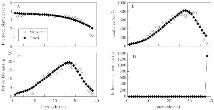
Figure 7 presents a comparison between the observed and fitted data for a sunflower plant that had completed 60 GCs. A satisfactory fit was obtained for the internode diameter (Fig. 7A), leaf blade surface area (Fig. 7B), petiole fresh weight (Fig. 7C) and fresh weight of the inflorescence (Fig. 7D). The degree of stability of these parameters across different environments, however, remains to be tested.
Fig. 7. Measured and fitted results for sunflower plants having completed 60 GCs.
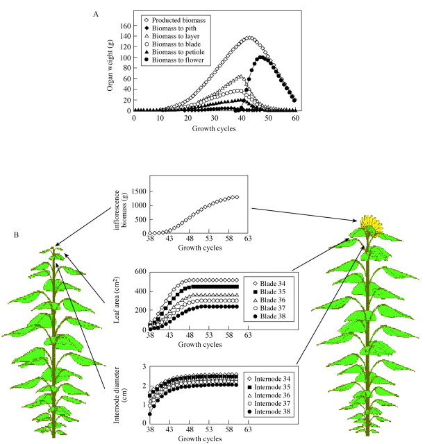
Figure 8 shows simulated biomass assimilation and partitioning patterns of sunflower, as well as the visualized plant. The biomass partitioned to leaf and internodes increases until flowering because biomass production increases, but decreases thereafter because of competition from the inflorescence. This results in classical features such as exponential growth followed by linear growth and, as leaf production ceases, decreasing growth rates. During the final cycles, no more biomass is partitioned to leaf blades and relatively little to the internode pith, due to a dominant inflorescence sink. Consequently, leaf blades stop growing but the diameter of internodes still increase because of the addition of new layers. Note that the model thereby simulated correctly the variation in leaf size despite the use of constant parameters.
Fig. 8. (A) Biomass production and partitioning kinetics simulated after fitting GREENLAB to a sunflower target data file. (B) Simulated organ expansion kinetics and 3D visualization of sunflower at 38 and 60 GCs.
Simulating morphological plasticity caused by sink or source manipulations
Although calibration of GREENLAB is based on fitting parameters to a specific target plant, it is possible subsequently to simulate different morphologies (but, at this point, not different architectures) using the same parameters but different resource situations. The resulting morphological plasticity has the same physiological basis as the variability of leaf size described above for a sunflower shoot. Similarly, the model is able to simulate compensatory growth after pruning, as illustrated in Fig. 9 for cotton (de Reffye et al., 1999). Both the real and the virtual plants responded to removal of branches by producing a taller plant bearing larger leaves, but less total biomass. Similarly, different levels of pruning of flower buds on virtual plants leads to strong variations in total biomass production and harvest index, enabling the optimization of source–sink relations (data not presented).
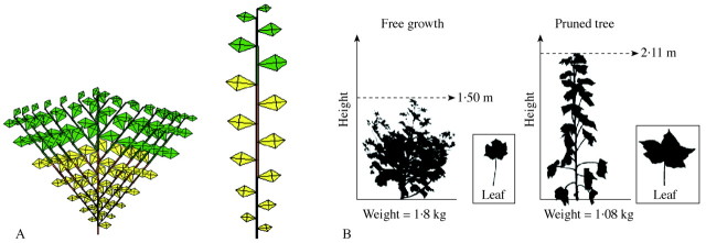
Fig. 9. Effect of branch pruning on cotton, (A) simulation, (B) observation. Suppressing axillary buds increases the size of phytomers but reduces overall plant size.
PERSPECTIVES
The simulations demonstrate the potential of mathematical, architectural models to incorporate some physiological aspects of plant functioning, and thereby go significantly beyond a mere reconstruction of a complex object. In particular, this approach allows the representation of variable organ size despite constant, ‘genetic’ parameters, on the basis of a very simple notion of competition among sinks. The model in its present form, however, over‐simplifies a number of processes, such as photosynthesis and assimilate conversion to biomass, and is not able to take into account important resources such as water. The root system is not yet represented, and light harvesting is at this stage insensitive to shading within and among plants. A new version of the model having such features is near completion and will be presented shortly.
Conceptually more important than these issues are two interrelated questions: to what extent can mathematical models, in contrast to classical, discrete‐event based crop models, handle plant responses to variable environments? And can such models, which are demonstrably good at ‘recreating’ an observed organism, be used to extrapolate plant behaviour beyond the observed situation? Mathematical models are potentially able to simulate the range of morphological and architectural variation, or plasticity, that results from a single set of ‘genetic’ parameters and parameter relationships that are in force throughout the plant’s life cycle, but not the intermittent switching on and off of rules, or the modification of rules or parameters. From a genetic perspective, the mathematical model would be able to simulate the constitutive features of the plant but not, or poorly, its inducible features. This may restrict to some extent the model’s capacity to simulate phenotypic plasticity (Nelson, 2000). In other words, any adaptive behaviour of the phenotype simulated by the model will function as an inherent feature of the system, and not as a discontinuity in the application of rules.
A next step towards the simulation of true phenotypic plasticity in terms of a variable body plan (Dewitt and Scheiner, 2003) will be the inclusion of feedbacks of resources on architecture, in addition to the feedbacks on geometry as simulated with the current model. Dusserre et al. (2002) recently demonstrated that cotton plants do not only adjust final organ size to the level of competition among assimilate sinks, but also adjust organogenesis (appearance rate of phytomers) and the period of organ expansion (filling duration). A version of GREENLAB is in progress that simulates resource‐dependent phenology and architecture on this basis.
In terms of applications, the model targets users who need to represent or predict 3D plant structure as a function of environment and management factors. This includes, among other things, the simulation of hypothetical ideotypes of crops or ornamentals (Dingkuhn et al., 1991; Yina et al., 2000), the optimization of phenotypes through pruning and crop/resource management, or the study of interactions between members of a plant community in space and time.
CONCLUSIONS
In this paper, we introduced a new, mathematical plant growth model that integrates complex architectural and morphological features with biomass production and allocation. The model is extremely simple in its physiological components, and therefore at present mainly suited to perform conceptual studies, but has the potential of becoming a fully quantitative tool. Although calibrated by optimization to reconstruct observed, prototypic plants, the model is able to simulate some of the plant’s phenotypic plasticity resulting from competition among sinks for resources. This, as well as the dynamic simulation of complex morphogenetic processes using the principle of sub‐structures, constitutes important innovations in plant architectural modelling.
The future challenges confronting this approach will be (1) the need to substitute some of the lumped functions (black boxes) with mechanistic processes, such as energy interception and conversion, and water status dynamics and their physiological feedbacks on plant growth; (2) the formulation of feedbacks of physiological status on architecture, in addition to plant geometry; and (3) the demonstration that the resulting system is useful not only for the recreation of observed structures (representation, explanation) but also for the accurate prediction of phenotypes in hypothetical environments (extrapolation).
Acknowledgements
The authors wish to thank Dr Hu Bao Gang, director of the LIAMA laboratory at Beijing, for having hosted and supported much of this work, Drs Guo Yan and Zhang Bao Gui, scientists of the China Agricultural University, for having contributed to this research, the National Scientific Foundation of China (NSFC) and the Ministry of Research for financial support.
Received: 12 September 2003; Returned for revision: 24 October 2003; Accepted: 7 January 2004 Published electronically: 31 March 2004
References
- AllenRG,PereiraLS,Raes D,SmithM.1998.Crop evapotranspiration. Guidelines for computing crop water requirements. FAO Irrigation and Drainage Paper No. 56, Rome: FAO, 299 pp. [Google Scholar]
- BaoGH, de Reffye P, Zhao X, Hong PY, Meng ZK.2003. Greenlab: a new methodology towards plant structural‐functional model – structural aspect. In: Bao GH, Jaeger M, eds. Proceedings of ‘plant growth modeling and applications’ (PMA’03), Beijing, China, 13–16 October 2003, Beijing: Tsinghua University Press and Springer, 21–35. [Google Scholar]
- BrissonN,Ruget F, Gate P, Lorgeau J, Nicoullaud B, Tayot X, Plénet D, Jeuffroy MH, Bouthier A, Ripoche D, Mary B, Justes E.2002. STICS: a generic model for simulating crops and their water and nitrogen balances. 2. Model validation for wheat and maize. Agronomie 22: 69–92. [Google Scholar]
- BakerDN, Lambert JR, McKinion JM.1983. Gossym: a simulator of cotton crop growth and yield. South Carolina Agricural Experimental Station Technical Bulletin 1089: 1–134. [Google Scholar]
- ChelleM. Andrieu B.1998. The nested radiosity model for the distribution of light within plant canopies. Ecological Modelling 111: 75–91. [Google Scholar]
- DauzatJ.1994. Radiative transfer simulation on computer models of Elaeis guineensis Oléagineux 49: 8–90. [Google Scholar]
- DauzatJ, Eroy MN.1997. Simulation light regime and intercrop yields in coconut based farming systems. European Journal of Agronomy 7: 63–74. [Google Scholar]
- DewittTJ, Scheiner SM (eds.)2003.Phenotypic plasticity. Functional and conceptual approaches. New York: Oxford Life Sciences, 272 pp. [Google Scholar]
- DingkuhnM, Miezan KM.1995. Climatic determinants of irrigated rice performance in the Sahel. II. Validation of photothermal constants and characterization of genotypes. Agricultural Systems 48: 411–434. [Google Scholar]
- DingkuhnM, Penning de Vries FWT, De Datta SK, van Laar HH.1991. Concepts for a new plant type for direct seeded flooded tropical rice. In: Direct seeded flooded rice in the tropics Manila, Philippines: International Rice Research Institute, 17–38. [Google Scholar]
- DusserreJ, Crozat Y, Warembourg FR, Dingkuhn M.2002. Effects of shading on sink capacity and yield components of cotton in controlled environments. Agronomie 22: 307–320. [Google Scholar]
- GaoL, Jin Z, Huang Y, Zhang L.1992. Rice clock model – a computer model to simulate rice development. Agriculture and Forest Meteorology 60: 1–16. [Google Scholar]
- GuoY, de Reffye P, Song YH, Zhan ZG, Li BG, Dingkuhn M.2003. Modeling of biomass acquisition and biomass partitioning in the architecture of sunflower. In: Proceedings of the 2003 International Symposium on Plant Modelling, Simulation, Visualisation and their Applications (PMA′03), October 2003, Beijing, China (in press). [Google Scholar]
- HowellTA, Musick JT.1984. Relationship of dry matter production of field crops to water consumption. Les besoins en eau des cultures Conférence internationale, Paris, 11–14 Sept. Paris: INRA, 247–269. [Google Scholar]
- HsiaoTC, Xu LK.2000. Pedicting water use efficiency of crops. Acta Horticulturae 537: 199–206. [Google Scholar]
- JallasE, Martin P, Sequeira R, Turner S, Cretenet M, Gérardeaux E.2000. Virtual COTONS®, the firstborn of the next generation of simulation models. Virtual Worlds 2000: 235–244 [Google Scholar]
- JonesCA, Kiniry JR.1986.CERES‐Maize: A simulation model of maize growth and development. Texas: Texas A&M University Press. [Google Scholar]
- JonesJW, Tsuji GY, Hoogenboom G, Hunt LA, Thornton PK, Wilkens PW, Imamura DT, Bowen WT, Sing U.1998. Decision support system for agrotechnology transfer; DSSAT v3. In: G.Y. Tsuji, G. Hoogenboom and P.K. Thornton. Understanding options for agricultural production Dordrecht: Kluwer Academic, 157–177. [Google Scholar]
- KurthW, Sloboda B.1997. Growth grammars simulating trees‐an extension of L‐systems incorporating local variables and sensitivity. Silva Fennica 31: 285–295. [Google Scholar]
- LindenmayerA.1968. Mathematical models for cellular interaction in development, parts I and II. Journal of Theoretical Biology 18: 280–315. [DOI] [PubMed] [Google Scholar]
- MarcelisLFM, Heuvelink E, Goudriaan J.1998. Modelling biomass production and yield of horticultural crops: a review. Scientia Horticulturae 74: 83–111. [Google Scholar]
- McFersonJ, Pierce F.2003.Technology roadmap. Research priorities to enhance tree fruit production through technological innovation Wenatchee WA, USA: Washington Tree Fruit Commission, www.treefruitresearch.org [Google Scholar]
- NelsonCJ.2000. Shoot morphological plasticity of grasses: leaf growth vs. tillering. In: Lemaire G, Hodgson J, Moraes A, de Cavalho PC, Nabinger C, eds. Grassland ecophysiology and grazing ecology Wallingford, UK: CABI Publishing, pp. 101–126. [Google Scholar]
- PerttunenJ, Sievänen R, Nikinmaa E, Salminen H, Saarenmaa H, Väkevä J.1996. LIGNUM: a tree model based on simple structural units. Annals of Botany 77: 87–98. [Google Scholar]
- PrakashCS.2001. The genetically modified crop debate in the context of agricultural evolution. Plant Physiology 126: 8–15. [DOI] [PMC free article] [PubMed] [Google Scholar]
- PrusinkiewiczP, Lindenmayer A, Hanan J.1988. Developmental models of herbaceous plants for computer imagery purposes. Computer Graphics 22: 141–150. [Google Scholar]
- de ReffyeP, Edelin C, Francon J, Jaeger M, Puech C.1988. Plant models faithful to botanical structure and development. Computer Graphics 22: 151–158. [Google Scholar]
- de ReffyeP, Blaise F, Chemouny S, Jaffuel S, Fourcaud T, Houllier F.1999. Calibration of hydraulic growth model on the architecture of cotton plants. Agronomie 19: 265–280. [Google Scholar]
- SievanenR, Nikinmaa E, Nygren P, Ozier‐Lafontaine H, Perttunen L, Hakula H.2000. Components of functional‐structural tree models. Annals of Forestry Science 57: 399–412. [Google Scholar]
- SmithAR.1984. Plants, fractals and formal languages. Computer Graphics 18: 1–10. [Google Scholar]
- StanhillG 1986. Water use efficiency. Advances in Agronomy 39: 53–85. [Google Scholar]
- XingZ, de Reffye P, Barthélémy D, Bao GH.2003. Interactive simulation of plant architecture based on a dual‐scale automaton model. In: Bao GH, Jaeger M, eds. Proceedings of ‘plant growth modeling and applications’ (PMA’03), Beijing, China, 13–16 October 2003, Beijing: Tsinghua University Press and Springer, 144–153. [Google Scholar]
- YanHP, Barczi J‐F, de Reffye Ph, Hu BG.2002. Fast algorithms of plant computation based on substructure instances. International Conferences in Central Europe on Computer Graphics, Visualization and Computer Vision 10: 145–153. [Google Scholar]
- YinaX, Kropff MJ, Goudriaan J, Stam P.2000. A model analysis of yield differences among recombinant inbred lines in barley. Agronomy Journal 92: 114–120. [Google Scholar]
- ZhanZhG. Wang YM, de Reffye Ph, Wang BB, Xiong YW.2002.Architectural modeling of wheat growth and validation study. 2000 ASAE Annual International Meeting, July 2000. [Google Scholar]


