Some Quantitative Relationships between Leaf Area Index and Canopy Nitrogen Content and Distribution

Abstract

In a previous study (Yin et al. 2000. Annals of Botany 85: 579–585), a generic logarithmic equation for leaf area index (L) in relation to canopy nitrogen content (N) was developed: L=(1/k_tn)1n(1+k_tnN/n_b). The equation has two parameters: the minimum leaf nitrogen required to support photosynthesis (n_b), and the leaf nitrogen extinction coefficient (k_tn). Relative to n_b, there is less information in the literature regarding the variation of k_tn. We therefore derived an equation to theoretically estimate the value of k_tn. The predicted profile of leaf nitrogen in a canopy using this theoretically estimated value of k_tn is slightly more uniform than the profile predicted by the optimum nitrogen distribution that maximizes canopy photosynthesis. Relative to the optimum profile, the predicted profile is somewhat closer to the observed one. Based on the L–N logarithmic equation and the theoretical k_tn value, we further quantified early leaf area development of a canopy in relation to nitrogen using simulation analysis. In general, there are two types of relations between L and N, which hold for canopies at different developmental phases. For a fully developed canopy where the lowest leaves are senescing due to nitrogen shortage, the relationship between L and N is described well by the logarithmic model above. For a young, unclosed canopy (i.e. L < 1·0), the relation between L and N is nearly linear. This linearity is virtually the special case of the logarithmic model when applied to a young canopy where its total nitrogen content approaches zero and the amount of nitrogen in its lowest leaves is well above n_b. The expected patterns of the L–N relationship are discussed for the phase of transition from young to fully developed canopies.

INTRODUCTION

Leaf area index (L, see Table 1 for abbreviations) of a canopy is an important variable in models for predicting crop growth and yields, quantifying crop–weed competition, or modelling heat, energy and water exchanges in the plant–soil–atmosphere continuum. Empirical data have shown that nitrogen is an important factor affecting crop L, either for early stages (Zhong, 1999) or for the whole growth season (Booij et al., 1996). Theoretical optimization analysis (Anten et al., 1995b; Goudriaan, 1995; Hirose et al., 1997) has also shown that canopy nitrogen content (N), the amount of nitrogen in all the leaves of a canopy, is a major determinant of optimum crop L (L_opt) for the maximized canopy photosynthesis. However, little attention has been paid to the effect of nitrogen on L in crop modelling research. Early models (e.g. Penning de Vries et al., 1989) predict L from leaf biomass using the parameter specific leaf area (s_la), assuming that leaf area is limited only by assimilate or carbon supply. More recently, leaf area was described to switch from temperature to carbon limitation: the daily increase in L (ΔL) is calculated first as a function of temperature up to a specific L, and then in proportion to the increment of leaf biomass (Goudriaan and van Laar, 1994). Van Delden et al. (2001) evaluated this two‐phase approach and found that it described field‐observed L better than when based solely on carbon supply or temperature. However, this approach assumes that temperature is the overwhelming determinant of L when the canopy is open, ignoring any effect of factors such as nitrogen, radiation and CO₂.

Table 1.

List of abbreviations

Symbol	Definition	Unit
k en	Extinction coefficient for effective leaf nitrogen	m2 ground m–2 leaf
k tn	Extinction coefficient for total leaf nitrogen	m2 ground m–2 leaf
k r	Extinction coefficient for PAR	m2 ground m–2 leaf
L	Leaf area index	m2 leaf m–2 ground
L i	L counted from the top to the i‐th layer of canopy	m2 leaf m–2 ground
L opt	Optimum L for maximal canopy photosynthesis	m2 leaf m–2 ground
n	The amount of nitrogen per unit leaf area	g N m–2 leaf
n n̄	The average value of n in canopy	g N m–2 leaf
n b	The base value of n for photosynthesis	g N m–2 leaf
n bot	n for the bottom leaves of canopy	g N m–2 leaf
n i	n for the i‐th layer leaves from the top of canopy	g N m–2 leaf
n o	n for the top leaves of canopy	g N m–2 leaf
N	Canopy nitrogen content	g N m–2 ground
P max	Leaf photosynthesis under saturated light conditions	e.g. g CO2 m–2 leaf s–1
s la	Specific leaf area	m2 leaf g–1 leaf mass
Δnbot	Rate of change in nbot	g N m–2 leaf d–1
ΔL	Rate of change in L	m2 leaf m–2ground d–1
ΔN	Rate of change in N	g N m–2 ground d–1
Δt	Time step in dynamic simulation	d

In fact, the effect of nitrogen on leaf area of a canopy in the later stages of growth of agricultural crops is well understood. The withdrawal of leaf nitrogen seems to be inevitable so as to support seed filling, because actual nitrogen uptake in later growth stages may not be sufficient to meet the high nitrogen demand required to build seed proteins (Sinclair and de Wit, 1975, 1976). This withdrawal causes leaf senescence, and crop L declines accordingly, a phenomenon described by Sinclair and de Wit (1975) as ‘self destruction’.

It has been observed in various species that total leaf nitrogen per unit leaf area (leaf nitrogen, hereafter) is not uniform at different heights of a canopy, but declines gradually over its depth (Field, 1983; Hirose and Werger, 1987; Evans, 1993). This non‐uniform vertical distribution of leaf nitrogen (n) is commonly described by:

where n_i is the leaf nitrogen of the i‐th layer of the canopy, where L counted from the top is L_i, n_o is the leaf nitrogen at the top of the canopy (i.e. at L_i = 0), and k_tn is the extinction coefficient of n. Starting with eqn (1), Yin et al. (2000) derived a generic equation for nitrogen‐limited leaf area index (Appendix):

where n_b is the base value of n, at or below which photosynthesis under saturated light conditions (P_max) is zero, reflecting photosynthetically inactive nitrogen components. This base value, as shown by experimental measurements that relate P_max directly to n (e.g. Evans, 1983; Sinclair and Horie, 1989; Anten et al., 1995a; Connor et al., 1995), varies from 0·1 to 1·0 g m^–2, depending on species and measurement conditions. Equation (2) can only be used to estimate L after the onset of leaf senescence. Before that moment, the leaf nitrogen of the bottom leaf (n_bot) is higher than n_b. Equation (2) will therefore overestimate the real L if applied to stages prior to that moment. This forms the basis for a biologically coherent approach to modelling both the timing and quantity of leaf senescence (Yin et al., 2000). However, whether or not eqn (2) represents the L–N relationship in an actual canopy has not yet been evaluated.

The application of eqn (2) requires an accurate estimate of its critical parameter k_tn, which may involve laborious measurements of n for leaves sampled at various heights of a canopy. Optimization for maximum canopy photosynthesis, achieved when no gain in canopy photosynthesis can be obtained by redistribution of nitrogen from one layer to another, may provide an alternative way to quantify the canopy nitrogen profile. If the relationship between P_max and n is linear, such an optimized canopy requires a vertical distribution of nitrogen such that the value of P_max in a layer is proportional to the mean absorbed photosynthetically active radiation (PAR) in that layer (Anten et al., 1995a; Goudriaan, 1995; Sand, 1995). The optimization theory has formed the basis of simple ‘big‐leaf’ analytical solutions for canopy photosynthesis (De Pury and Farquhar, 1997). Anten et al. (1995a) examined four contrasting species experimentally, and found that the pattern of n in the canopy was indeed mainly determined by the extinction coefficient for PAR (k_r). The observed decline of n over the depth of a canopy may reflect an acclimation of leaf nitrogen distribution at the canopy level (Schapendonk et al., 1999). Based on the optimization theory, one would assume that it is the effective leaf‐nitrogen, n – n_b, rather than n itself, which follows an exponential profile in the canopy (Sands, 1995):

where k_en is the extinction coefficient for the effective leaf nitrogen. If a canopy is entirely acclimated (i.e. the actual nitrogen profile follows exactly the optimum one), then k_en equals k_r. The advantage of using eqn (3) to describe the nitrogen profile then becomes immediately obvious, because k_r is more commonly measured as an input parameter in crop growth models. However, eqn (3) cannot be used as a basis to derive an equation similar to eqn (2) that links L with N, because eqn (3) predicts that the amount of nitrogen in the bottom leaves of a canopy can never be as low as n_b.

Given the importance of nitrogen in canopy development and maintenance, there is a need to establish quantitative relations between L and N during crop growth in order to model crop yields in relation to nitrogen. Optimization analysis (e.g. Goudriaan, 1995) does provide relationships for the dependence of L_opt on N. However, the calculated L_opt is of little use in numerical models for crop growth, because L_opt is a function not only of N but also of other variables such as PAR. A crop cannot adjust its L that fast in response to rapid fluctuation of PAR under field conditions. The objective of this paper is to provide a quantitative framework for calculating L in relation to N, for use in crop growth models. It is the follow‐up analysis of a previous report (Yin et al., 2000) in which a method was introduced for modelling leaf senescence in late growth stages, based on the profile of exponential decay of nitrogen in the canopy. Since eqn (2) is central to the whole analysis, we will first assess its ability to describe the relationship between L and N for established canopies. Given the need to measure the value of k_tn when using eqn (2) in crop modelling, we will then derive an equation to theoretically estimate its value from those variables that are either easier to measure or are commonly calculated in the models. Thirdly, we will use these relationships to quantify the effect of nitrogen on early leaf area development in young canopies. Finally, we will present the expected whole picture of the L–N relationship, covering canopies in the early, fully developed and in‐between transitional phases of development.

THEORY

Theoretical estimation of k_tn

If eqn (1) is applied to leaves in the bottom layer of a canopy, it can be rewritten as:

Based on eqn (3), the value of N can be solved analytically as:

Solving eqn (5) for n_o gives:

When equation (3) is applied to leaves in the bottom layer of a canopy it becomes:

Substituting n_o from eqn (6) into eqn (7) gives:

If canopy nitrogen is fully acclimated to follow the optimum profile, k_en in eqns (5)–(8) can be replaced with k_r (Kull and Javis, 1995), a commonly measured parameter in crop models. Substituting n_o and n_bot from eqns (6) and (8) into eqn (4) gives:

Obviously, whilst eqn (9) is derived using information on the optimum nitrogen distribution, it predicts a profile that differs from the optimum one (see the Results).

Quantifying early leaf area development

If applied to a developing canopy where the bottom leaves are still photosynthetically active, eqn (2) has to be written as:

where n_b in eqn (2) has been replaced by n_bot. In a young developing canopy, n_bot gradually decreases over time to approach n_b. Because n_bot is not constant, eqn (10) cannot be directly applied to a young canopy. We apply a dynamic simulation approach, where both L and N are described as state variables. The rate of change in L from one time step to another is calculated from a differential form of eqn (10):

where ΔN and Δn_bot are the rate of change in N and n_bot, respectively. ΔN is simply the current nitrogen uptake allocated to leaves. However, Δn_bot is unknown. To overcome this problem, n_bot is also described as a state variable. Its initial value is calculated from initial L and N using eqn (A3a). Δn_bot can then be calculated by:

where Δt is the time step of dynamic simulation. The first part of the numerator in eqn (12) is the expected value of n_bot based on eqn (A3a).

Equation (11) is a simplified differential form of eqn (10), assuming that k_tn does not change with time. This is in contrast to the prediction of eqn (9) that k_tn does change with time because both L and N change with time. However, simulations show that its change during the early growth stage is small (see Results). Thus, the more complex differential form assuming that k_tn changes with time is not applied here.

Equations (11) and (12) have been incorporated in the daily time‐step crop model of Yin et al. (2001), where the dynamics of ΔL are described in two phases. The first phase stops at the moment when L = 1·0 (Kropff et al., 1994). For this phase, our approach as given above [eqns (11) and (12)] has been implemented. The second phase then follows, predicting ΔL from s_la and the increment of leaf biomass. Because the use of eqn (11) involves nitrogen uptake, the relations for predicting crop nitrogen uptake in the model of Yin et al. (2001) are outlined in the Appendix.

RESULTS AND DISCUSSION

Ability of eqn (2) to describe the relationship between L and N in a full canopy

A fully developed crop canopy is defined here as a canopy in which leaf nitrogen of the bottom leaf has reached n_b. For such a canopy, eqn (2) is valid. Two data sets were used to test the ability of eqn (2) to represent the relationships between L and N in such a canopy. The first data set involved canopies at four seed‐filling stages of sunflower (Helianthus annuus L.) grown at two densities and with different nitrogen supplies (Connor et al., 1995). The second one was taken from field experiments with wheat crops conducted over two seasons at three locations (Groot and Verberne, 1991). Only measurements made after the onset of leaf senescence are used here.

For both data sets, the relationship between L and N did not differ among treatments (Fig. 1A) or among locations (Fig. 1B). Therefore, data points were pooled. Observations from different sampling times in each data set seemed to follow the same pattern. Equation (2) described the curvilinear relationships well. The logarithmic relationship implies that n declines gradually towards maturity, as shown by the shape of the curve close to the origin of coordinates. The estimates for k_tn and n_b were 0·917 m² m^–2 and 0·537 g m^–2 for sunflower (Fig. 1A), and 0·464 m² m^–2 and 0·597 g m^–2 for wheat (Fig. 1B). Comparing the data sets, slightly more scatter was observed with wheat data, especially as canopy nitrogen content increased (Fig. 1B). The two obvious outliers are due to the high uptake of fertilizer nitrogen applied during the seed‐filling stage.

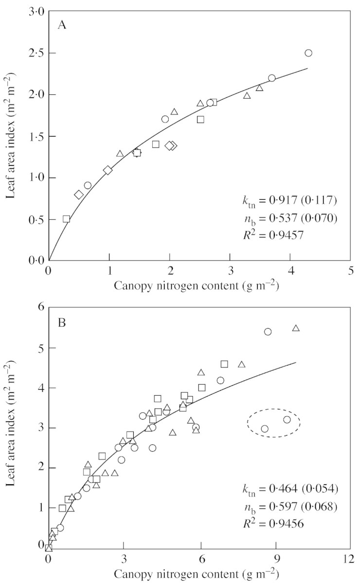
Fig. 1. Relationship between leaf area index and canopy nitrogen content for fully developed canopies, based on data of Connor et al. (1995) for sunflower ‘Prosol 35’ (A), and of Groot and Verberne (1991) for winter wheat ‘Arminda’ (B). Different symbols represent four different treatments (A) or three experimental locations (B). The two encircled points in B are outliers, resulting from a late application of nitrogen fertilizer. The curves represent eqn (2), with parameters (standard error in parentheses) fitted to all data points.

Equation (2) provides a simpler platform for estimating k_tn than does eqn (1), for which both L and n at different vertical layers of a canopy have to be measured. It can also be used to determine n_b, which is commonly estimated from extrapolating the fitted relationship between P_max and n. By using eqn (2), n_b can be obtained without the use of gas exchange equipment for measuring P_max. It should be noted that the accuracy of estimating n_b by using eqn (2) relies on judgement of whether yellowing leaves at the bottom of a canopy are still photosynthetically active. Our estimates of n_b are higher than reported values of n_b based on measuring leaf photosynthesis, i.e. 0·30 g m^–2 for sunflower (Connor et al., 1995) and 0·35 g m^–2 for wheat (Dreccer et al., 2000). This higher estimate is presumably due to the exclusion of those yellowing but still photosynthetically active leaves when measuring canopy L and N in the two experiments. No matter how n_b is estimated, the accuracy of its value is important since it affects the estimate of canopy nitrogen available for photosynthesis.

Estimation of k_tn using eqn (9)

Three data sets were used to evaluate the ability of eqn (9) to describe the canopy nitrogen profile. The first one came from Dreccer et al. (2000) for wheat grown with two levels of nitrogen and at two densities. Plants were grown in a hydroponics system that consisted of containers (25 l and 0·145 m² each) connected with pipelines. Plants were grown in three rows per container, shielded with an aluminium screen to avoid any bordering effect. Canopy nitrogen profile was measured 42, 64, 78 and 92 d after germination (DAG). The second data set refers to faba bean (Vicia faba L.) crops grown in the field in 1991 at two densities (Del Pozo and Dennett, 1999). Canopy nitrogen profile was measured on two dates: 12 and 29 July. The third data set was published for canopies of four contrasting species: rice, soybean [Glycine max (L.) Merr], sorghum (Sorghum bicolor L.) and amaranthus (Amaranthus cruentus L.) (Anten et al., 1995a). These data sets were chosen for our analysis because all the input variables (L, N) and input parameters (k_r, n_b) of eqn (9) are given in these reports or can be derived easily from the presented data (Table 2).

Table 2.

Estimation of leaf nitrogen extinction coefficient k_tn by eqn (9), and fitted values for k_tn and k_en

	L (m2 m–2)	N (g m–2)	kr (m2 m–2)	nb (g m–2)	ktn‐calculated (m2 m–2)*	ktn‐fitted (m2 m–2)†	ken‐fitted(m2 m–2)†
Dreccer et al. (2000)
LNLD42§	0·294	0·194	0·590	0·35	0·277	0·663	1·287
LNLD64	0·421	0·266	0·590	0·35	0·263	0·315	0·708
LNLD78	0·502	0·458	0·640	0·35	0·394	0·611	1·059
LNLD92	0·591	0·560	0·890	0·35	0·558	0·776	1·240
LNHD42	0·372	0·236	0·660	0·35	0·296	1·072	2·547
LNHD64	0·704	0·405	0·420	0·35	0·164	0·364	0·964
LNHD78	0·772	0·501	0·420	0·35	0·193	1·087	2·450
LNHD92	1·010	0·950	0·620	0·35	0·386	0·318	0·537
HNLD42	0·656	0·523	0·490	0·35	0·274	–0·142‡	–0·217‡
HNLD64	1·404	1·173	0·370	0·35	0·214	0·441	0·802
HNLD78	1·644	1·460	0·390	0·35	0·234	0·360	0·638
HNLD92	2·522	2·790	0·420	0·35	0·281	0·285	0·425
HNHD42	0·908	0·779	0·410	0·35	0·242	0·425	0·727
HNHD64	1·387	1·120	0·530	0·35	0·297	0·528	0·980
HNHD78	2·332	2·022	0·330	0·35	0·194	0·410	0·791
HNHD92	3·139	3·220	0·430	0·35	0·274	0·365	0·639
Del Pozo and Dennett (1999)
HD July12	6·800	9·861	0·655	0·66	0·264	0·193	0·472
HD July29	3·900	7·263	0·835	0·66	0·450	0·214	0·378
LD July12	3·250	5·722	0·927	0·66	0·494	0·305	0·591
LD July29	2·800	5·586	0·935	0·66	0·556	0·242	0·368
Anten et al. (1995a)
Oryza	5·480	6·320	0·469	0·36	0·288	0·115	0·175
Glycine	4·760	7·563	0·749	0·41	0·459	0·262	0·389
Sorghum	5·920	5·522	0·631	0·18	0·424	0·115	0·148
Amaranthus	4·990	5·905	0·779	0·35	0·435	0·297	0·462

* Calculated using eqn (9).

^† Fitted to the profile data using eqn (1) for k_tn and using eqn (3) for k_en.

^‡ Negative value due to small cloud of data points.

^§ HN, High nitrogen supply; LN, low nitrogen supply; HD, high density; LD, low density; the number following these codes refers to sampling time (days after germination).

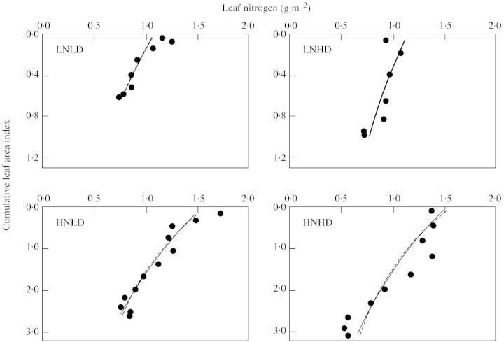
The canopy size of the crops reported by Dreccer et al. (2000) was generally small. For this data set, the combination of two nitrogen levels, two densities and four sampling times resulted in 16 sets of nitrogen profile (Table 2). Because the trend was similar, only profiles from the last sampling date (92 DAG) are visualized (Fig. 2). The profile predicted by eqn (1), using k_tn calculated from eqn (9), is close to that predicted from the optimum distribution, i.e. eqn (3) where k_en is set to k_r. Both predictions are slightly more uniform than, but similar to, the actually measured profile.

Fig. 2. Leaf nitrogen distribution in spring wheat crops (‘Minaret’) grown at low nitrogen supply (LN) and low density (LD), or LN and high density (HD), or high nitrogen (HN) and LD, or HN and HD, based on data of Dreccer et al. (2000). The full and broken curves represent the nitrogen profile predicted by eqn (1) with k_tn calculated from eqn (9), and the profile predicted by the optimum distribution [eqn (3) with k_en = k_r], respectively. Values of k_r and calculated k_tn are given in Table 2.

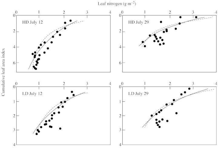
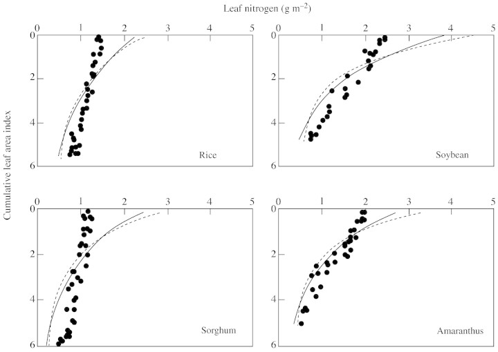
For the data sets of Del Pozo and Dennett (1999) and Anten et al. (1995a), larger canopies were obtained (Table 2; Figs 3 and 4). The observed profiles, especially those reported by Anten et al. (1995a), were more uniform than those predicted by using either k_tn [eqn (9)] or the optimum distribution (Table 2; Figs 3 and 4). Comparing the two predictions, profiles based on eqn (9) were somewhat more uniform and, therefore, slightly closer to the observed profiles (Figs 3 and 4).

Fig. 3. Leaf nitrogen distribution in faba bean crops (‘Tina’) grown at two densities [low (LD) and high (HD)], sampled at two dates (12 and 29 July), based on data of Del Pozo and Bennett (1999). Further details are as for Fig. 2.

Fig. 4. Leaf nitrogen distribution in four species, based on data of Anten et al. (1995a). Further details are as for Fig. 2.

Whilst eqn (9) uses four inputs (L, N, k_r and n_b) to calculate k_tn, it shows that k_r is the most important in determining k_tn (Fig. 5), in line with the conclusion that the pattern of canopy nitrogen allocation depends mainly on the extinction coefficient for PAR (Anten et al., 1995a). Values of k_tn calculated by eqn (9) are always lower than the observed k_r (Table 2), a finding that seems to be supported by some experimental reports (e.g. Sadras et al., 1993; Del Pozo and Dennett, 1999). Compared with the values of k_tn fitted to the actual data, the calculated k_tn is generally smaller for the data set of Dreccer et al. (2000) and is consistently greater for the other two data sets (Table 2). Because the optimum nitrogen distribution requires k_en, not k_tn, to equal k_r, values of k_en were also examined. In contrast to the consistent relationship k_en = 0·4k_r proposed by Anten (1997), fitted values of k_en in our analysis varied considerably among data sets and were greater than k_r in the data set of Dreccer et al. (2000) and smaller than k_r for the other two data sets (Table 2). Relative to fitted values of k_tn, those of k_en are consistently higher. This difference between k_en and k_tn arises from non‐photosynthetic nitrogen that is reflected by the positive value of n_b.

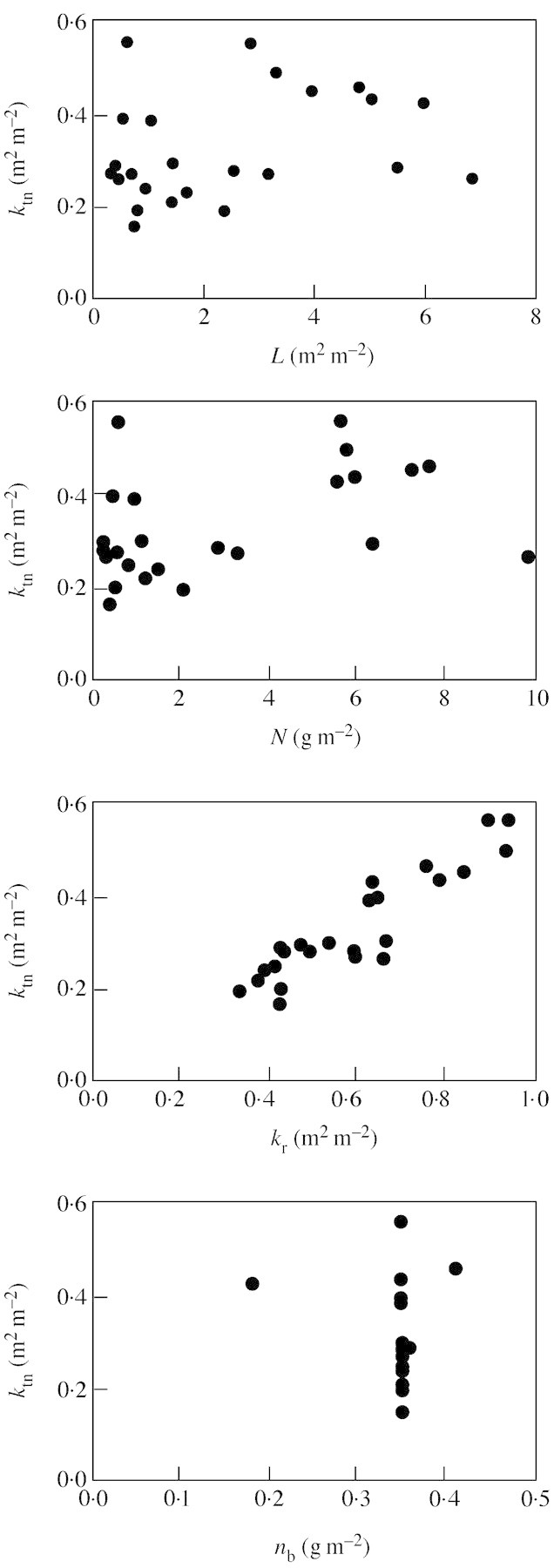
Fig. 5. Illustration of the effect of four independent variables (L, N, k_r and n_b) on the dependent variable k_tn in eqn (9) (data from Table 2).

The above results indicate that the nitrogen profile in an actual canopy, though acclimated to its light profile, may not reach a theoretical optimum. In particular, the observed nitrogen profiles are apparently more uniform than those predicted for large canopies (Figs 3 and 4). One or more of the following reasons could explain this. First, the optimum distribution theory is based on the assumption that the relationship between P_max and n is linear (Anten et al., 1995a; Goudriaan, 1995; Sand, 1995). However, the observed relationship is often non‐linear (e.g. Evans, 1983; Sinclair and Horie, 1989; Connor et al., 1995; Del Pozo and Dennett, 1999; Vos and van der Putten, 2001). Yin et al. (2000) inferred that compared with the linearity, the non‐linearity between P_max and n would require a more uniform nitrogen profile for the optimum acclimation. Secondly, the exponential profile of PAR penetration through a canopy holds best for diffuse light. In an actual canopy under natural growing conditions, some sunlight flecks penetrate even to the lowest leaves (De Pury and Farquhar, 1997). The light‐induced nitrogen acclimation, if the direct PAR received by lower leaves is considered, can result in a more uniform nitrogen profile than that predicted by the exponential light profile. This may explain the apparent disparity between theoretical and actual profiles in Fig. 4, as the PAR profile in this case was measured on overcast days (Anten et al., 1995a). Other non‐acclimation factors may affect nitrogen profile. For example, Sadras et al. (1993) and Bindraban (1999) observed a decline in leaf nitrogen in upper leaves, relative to lower leaves, during seed filling, possibly because of withdrawal of more nitrogen in upper than lower leaves to support seed filling because upper leaves are closer to the seeds.

Simulation analysis of early leaf area development

Equation (9) was incorporated into the crop growth model of Yin et al. (2001). Because k_r is the most important parameter determining k_tn (Fig. 5), a simulation was conducted by varying k_r within a common range, i.e. between 0·3 and 0·9 m² m^–2 (Table 2). Initial values for L and N in the simulation were taken from data of Groot and Verberne (1991) for winter wheat.

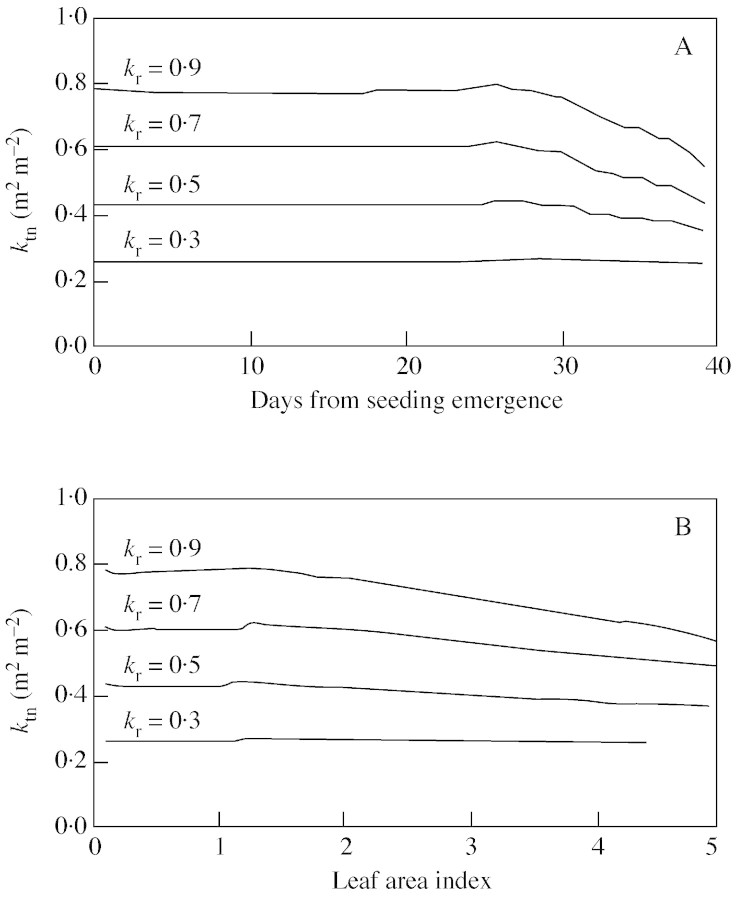
The simulation shows that the predicted k_tn at a certain k_r did not vary much in the early development stage (Fig. 6A). A reasonable threshold for the end of this early stage is when L equals 1·0 m² m^–2 (Fig. 6B). As k_r itself can be assumed to have a stable value during the early growth period (Kropff et al., 1994), it follows that k_tn varies little during the early phase. Therefore, eqn (11), the simplified differential form of eqn (10) assuming that k_tn is constant, can be used effectively for simulating crop leaf area development when L is less than 1·0.

Fig. 6. Simulated k_tn plotted against days from seedling emergence (A), or leaf area index (B), at four different values of k_r.

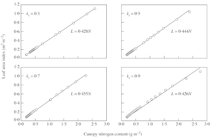
The predicted relationship between early L and N is nearly linear, and the slope of this linearity varies little with changing k_r (Fig. 7). The inverse of the slope of the linearity is the estimated average leaf nitrogen of canopy (n̄) during this early period. The prediction of L–N proportionality for early stages is not surprising because, for the very early period, the term k_tnN/n_bot in eqn (10) is very small, and eqn (10) becomes: , as it can be mathematically proven that e^x ≈ 1+x if x→ 0. Two main factors are responsible for the value of k_tnN/n_bot being small for the early stages: first, N itself is small during the early period, and secondly, n_bot is relatively large, nearly equivalent to nn̄.

Fig. 7. The simulated relationship between early leaf area index (L) and canopy nitrogen content (N) for winter wheat, using four different values of k_r. The line is the fitted relationship to the simulated values (points).

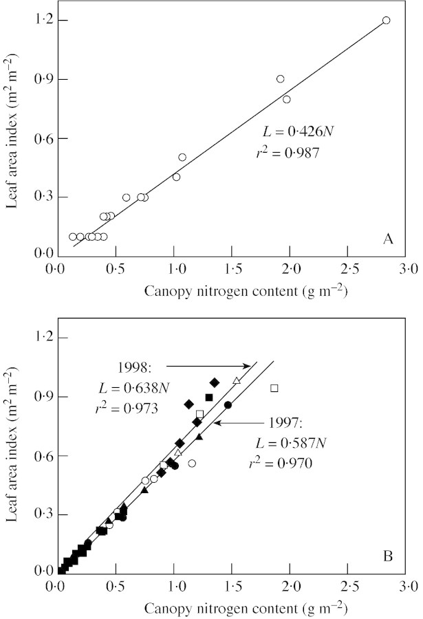
The linear relationship between L and N has been observed experimentally, across a range of nitrogen environments (Grindlay, 1997). Using the data of Groot and Verberne (1991) for winter wheat, we found a linear L–N relationship for the early growth period (Fig. 8A), with a similar slope value as predicted by our approach. Based on the data of Zhong (1999) for transplanted rice, a similar linearity was found (Fig. 8B). The difference between the two crops is a higher slope, i.e. a lower early nn̄ in rice, presumably due to the effect of transplanting in rice and/or differences in the growing environment between the two crops. In rice, the difference in the slope between 2 years or among treatments within a year is only slight (Fig. 8B).

Fig. 8. The observed relationship between early leaf area index, L, and canopy nitrogen content, N, for winter wheat ‘Arminda’ (data of Groot and Verberne, 1991) (A), and for rice ‘IR72’ (data of Zhong, 1999) (B). The line is the fitted relationship to the observed values (points). Data points for rice come from experiments in 2 years (open symbols for 1997, closed symbols for 1998), and the different symbols refer to four levels of treatment (1997, row spacing; 1998, amount of nitrogen applied).

The good agreement between simulated and measured L–N linearity for the early growth phase indicates that our analysis may provide a new avenue for robust dynamic modelling of early canopy development. Although our analysis is only approximate because of a delay of one time‐step in obtaining n_bot and Δn_bot, it overcomes the weakness of the solely temperature‐based approach that ignores any effect of other factors, such as nitrogen, radiation and CO₂. The present analysis assumes that nitrogen drives early leaf area development. Thus, the effect of nitrogen on L in the first phase can be seen directly from eqn (11). The effect of temperature, radiation and CO₂ in our analysis is implicit, i.e. through their effect on photosynthesis that affects shoot activity and consequently nitrogen uptake (Appendix).

Expected pattern of the L–N relationship for the mid‐phase

The proportionality of the L–N relationship during early crop development implies that the temporal change of nn̄ is negligible during this early phase. Whilst the formula L=N/nn̄ per se holds for any stage of a canopy, extension of the L–N linearity to a later stage (e.g. Booij et al., 1996) should be done with great caution. In fact, many experimental observations (e.g. Kropff et al., 1994) have shown that nn̄ declines with increasing L at later stages.

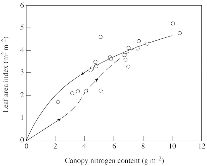
Beyond the early phase, the L–N relationship may be inferred by comparing the early linearity with the logarithmic pattern in the senescence phase. In Fig. 9, the early linear and the late logarithmic patterns are re‐plotted for the winter wheat data set of Groot and Verberne (1991), for which both relationships have been analysed in this paper. Clearly, there is a shortfall or gap between the linear and the logarithmic patterns. This gap could be filled by a third formula. However, it is difficult to derive a concrete form of such a formula using nitrogen‐based quantitative relationships presented in this paper. Our reasoning is that if the temporal trend of L during the early and the late phases is considered as nitrogen‐driven and nitrogen‐limited, respectively, the mid‐phase leaf area development could be carbon‐driven, letting nn̄ deviate from the initial constant until the lowermost leaves start to senesce. Such a consideration results in a mid‐phase L–N pattern that connects the linear and logarithmic curves (Fig. 9), and agrees with the assumption in models such as SUCROS (Goudriaan and van Laar, 1994), where ΔL after the initial development phase is estimated from s_la and the increment of leaf biomass. How fast it deviates from the initial linearity and where it meets the senescence‐phase curve may depend on a number of factors, such as genotype and interim nitrogen fertilization. The scatter in the experimental observations for the mid‐phase in Fig. 9 was probably due to the effect of both timing and quantity of nitrogen fertilization on the L–N relationship in this phase.

Fig. 9. Relationship between leaf area index (L) and canopy nitrogen content (N) for the early phase (the full line re‐plotted from Fig. 8A) and for the late senescence phase (the logarithmic curve re‐plotted from Fig. 1B), and the expected L–N relationship for the mid‐development phase (dashed curve). Points are from the mid‐phase samplings in the fertilizer experiments of Groot and Verberne (1991). Arrows indicate the temporal direction of L or N in the three phases.

CONCLUSIONS

In this paper, some quantitative relationships between L and N are presented, based on existing understanding of the exponential nitrogen distribution within the canopy. Three canopy development phases were distinguished. For a fully developed canopy, where the lowest leaves are senescing due to nitrogen shortage, the relationship between L and N is well described by a logarithmic model. For a young, unclosed canopy (i.e. L < 1·0), the relationship between L and N is virtually linear, a finding based on simulation analysis using simple modules for canopy photosynthesis and nitrogen uptake. For the intermediate phase, the relationship depends on factors such as fertilization regime, but a transition from the linear to the logarithmic pattern is expected. These phasic modes of canopy development could be the consequence of nitrogen‐driving, carbon‐driving and nitrogen‐limitation, respectively. The present analysis, combined with a previous report (Yin et al., 2000), may then result in a phasic canopy development model for predicting the temporal course of crop L, based on the concept of carbon–nitrogen interaction. This phasic canopy development model allows a robust prediction of leaf area index in a general crop growth model.

ACKNOWLEDGEMENTS

This work was supported partly by ‘De Technologiestichting STW’ part of the Netherlands Organisation for Scientific Research through the PROFETAS (PROtein Foods, Environment, Technology, And Society) programme of Wageningen University, and partly by the European Commission Environment & Change Programme via the MAGEC (Modelling Agroecosystems under Global Environmental Change) project (ENV4‐CT97‐0693) of Plant Research International. We thank Drs J. Vos and P. S. Bindraban for commenting on the manuscript.

APPENDIX

Derivation of eqn (2) as given by Yin et al. (2000)

The total amount of canopy nitrogen can be solved from eqn (1) as:

Solving eqn (A1) for n_o and substituting it into eqn (1) gives:

The amount of nitrogen in bottom leaves of a canopy, n_bot, can be formulated from eqn (A2) as:

For a fully developed canopy whose bottom leaves are senescing, n_bot is equal to n_b. Equation (A3a), if applied to this full canopy, becomes:

Solving eqn (A3b) for L gives eqn (2).

Relationships for nitrogen uptake in the crop model of Yin et al. (2001)

In the model of Yin et al. (2001), crop nitrogen uptake is determined as the minimum of nitrogen demand (N_dem) and nitrogen availability. N_dem was simulated based on the assumption that a crop takes up nitrogen in order to achieve the optimum nitrogen concentration that maximizes its relative growth rate (Hilbert, 1990):

where W_R is root biomass (g DM m^–2), σ_N is specific root activity (g N g^–1DM d^–1), σ_C is specific shoot activity (g C g^–1DM d^–1), which is crop net carbon fixation divided by shoot biomass, f_C is carbon fraction in biomass (g C g^–1DM), and F_N is whole plant nitrogen concentration (g N g^–1DM). Crop net carbon fixation is calculated according to Rodriguez et al. (1999). The term dσ_C/dF_N in eqn (A4) is given by:

where ΔF_N is a small increment of F_N, and σ_C(FN + Δ_FN) and σ_C(FN) are specific shoot activity when plant nitrogen fraction is F_N + ΔF_N and F_N, respectively.

Received: 20 November 2002; Returned for revision: 5 January 2003; Accepted: 28 February 2003    Published electronically: 15 April 2003

References

- AntenNPR.1997. Modelling canopy photosynthesis using parameters determined from simple non‐destructive measurements. Ecological Research 12: 77–88. [Google Scholar]
- AntenNPR, Schieving F, Werger MJA.1995a. Patterns of light and nitrogen distribution in relation to whole canopy carbon gain in C3 and C4 mono‐ and dicotyledonous species. Oecologia 101: 504–513. [DOI] [PubMed] [Google Scholar]
- AntenNPR, Schieving F, Medina E, Werger MJA, Schuffelen P.1995b. Optimal leaf area indices in C3 and C4 mono‐ and dicotyledonous species at low and high nitrogen availability. Physiologia Plantarum 95: 541–550. [Google Scholar]
- BindrabanPS.1999. Impact of canopy nitrogen profile in wheat on growth. Field Crops Research 63: 63–77. [Google Scholar]
- BooijR, Kreuzer ADH, Smit AL, van der Werf A.1996. Effect of nitrogen availability on dry matter production, nitrogen uptake and nitrogen interception of Brussels sprouts and leeks. Netherlands Journal of Agricultural Science 44: 3–9. [Google Scholar]
- ConnorDJ, Sadras VO, Hall AJ.1995. Canopy nitrogen distribution and the photosynthetic performance of sunflower crops during grain filling – a quantitative analysis. Oecologia 101: 274–281. [DOI] [PubMed] [Google Scholar]
- Del PozoA, Dennett MD.1999. Analysis of the distribution of light, leaf nitrogen, and photosynthesis within the canopy of Vicia faba L. at two contrasting plant densities. Australian Journal of Agricultural Research 50: 183–189. [Google Scholar]
- De PuryDGG, Farquhar GD.1997. Simple scaling of photosynthesis from leaves to canopies without the errors of big‐leaf models. Plant, Cell and Environment 20: 537–557. [Google Scholar]
- DreccerMF, van Oijen M, Schapendonk AHCM, Pot CS, Rabbinge R.2000. Dynamics of vertical leaf nitrogen distribution in a vegetative wheat canopy: impact on canopy photosynthesis. Annals of Botany 86: 821–831. [Google Scholar]
- EvansJR.1983. Nitrogen and photosynthesis in the flag leaf of wheat (Triticum aestivum L.). Plant Physiology 72: 297–302. [DOI] [PMC free article] [PubMed] [Google Scholar]
- EvansJR.1993. Photosynthetic acclimation and nitrogen partitioning within a lucerne canopy. II. Stability through time and comparison with a theoretical optimum. Australian Journal of Plant Physiology 20: 69–82. [Google Scholar]
- FieldC.1983. Allocating leaf nitrogen for the maximization of carbon gain: leaf age as a control on the allocation program. Oecologia 56: 341–347. [DOI] [PubMed] [Google Scholar]
- GoudriaanJ.1995. Optimization of nitrogen distribution and of leaf area index for maximum canopy assimilation rate. In: Thiyagarajan TM, ten Berge HFM, Wopereis MCS, eds. Nitrogen management studies in irrigated rice Los Baños, Philippines: International Rice Research Institute, 85–97. [Google Scholar]
- GoudriaanJ, van Laar HH.1994.Modelling potential crop growth processes. Dordrecht, The Netherlands: Kluwer Academic Publishers. [Google Scholar]
- GrindlayDJC.1997. Towards an explanation of crop nitrogen demand based on the optimization of leaf nitrogen per unit leaf area. Journal of Agricultural Science, Cambridge 128: 377–396. [Google Scholar]
- GrootJJR, Verberne ELJ.1991. Response of wheat to nitrogen fertilization, a data set to validate simulation models for nitrogen dynamics in crop and soil. Fertilizer Research 27: 349–383. [Google Scholar]
- HilbertDW.1990. Optimization of plant root:shoot ratios and internal nitrogen concentration. Annals of Botany 66: 91–99. [Google Scholar]
- HiroseT, Werger MJA.1987. Maximizing daily canopy photosynthesis with respect to the leaf nitrogen allocation pattern in the canopy. Oecologia 72: 520–526. [DOI] [PubMed] [Google Scholar]
- HiroseT, Ackerly DD, Traw MB, Ramseier D, Bazzaz FA.1997. CO2 elevation, canopy photosynthesis, and optimal leaf area index. Ecology 78: 2339–2350. [Google Scholar]
- KropffMJ, van Laar HH, Matthews RB.1994.ORYZA1: an ecophysiological model for irrigated rice production. Los Baños, Philippines: International Rice Research Institute. [Google Scholar]
- KullO, Jarvis PG.1995. The role of nitrogen in a simple scheme to scale up photosynthesis from leaf to canopy. Plant, Cell and Environment 18: 1174–1182. [Google Scholar]
- PenningdeVriesFWT, Jansen DM, ten Berge HFM, Bakema A.1989.Simulation of ecophysiological processes of growth in several annual crops. Wageningen, The Netherlands: Pudoc and Los Baños, Philippines: International Rice Research Institute. [Google Scholar]
- RodriguezD, van Oijen M, Schapendonk AHCM.1999. LINGRA‐CC: a sink‐source model to simulate the impact of climate change and management on grassland productivity. New Phytologist 144: 359–368. [Google Scholar]
- SadrasVO, Hall AJ, Connor DJ.1993. Light‐associated nitrogen distribution profile in flowering canopies of sunflower (Helianthus annuus L.) altered during grain growth. Oecologia 95: 488–494. [DOI] [PubMed] [Google Scholar]
- SandsPJ.1995. Modelling canopy production. I. Optimal distribution of photosynthetic resources. Australian Journal of Plant Physiology 22: 593–601. [Google Scholar]
- SchapendonkAHCM, van Oijen M, Pot SC, van den Boogaard R, Harbinson J.1999. Nitrogen shortage in a tomato crop; scaling up from effects of electron‐transport rate to plant productivity. Zeitschrift für Naturforschung 54c: 840–848. [Google Scholar]
- SinclairTR, de Wit CT.1975. Photosynthate and nitrogen requirements for seed production by various crops. Science 189: 565–567. [DOI] [PubMed] [Google Scholar]
- SinclairTR, de Wit CT.1976. Analysis of the carbon and nitrogen limitations to soybean yield. Agronomy Journal 68: 319–324. [Google Scholar]
- SinclairTR, Horie T.1989. Leaf nitrogen, photosynthesis, and crop radiation use efficiency: a review. Crop Science 29: 90–98. [Google Scholar]
- Van DeldenA, Kropff MJ, Haverkort AJ.2001. Modeling temperature‐ and radiation‐driven leaf area expansion in the contrasting crops potato and wheat. Field Crops Research 72: 119–142. [Google Scholar]
- VosJ, van der Putten PEL.2001. Effects of partial shading of the potato plant on photosynthesis of treated leaves, leaf area expansion and allocation of nitrogen and dry matter in component plant parts. European Journal of Agronomy 14: 209–220. [Google Scholar]
- YinX, Verhagen J, Jongschaap R, Schapendonk AHCM.2001.A model to simulate responses of the crop‐soil system in relation to environmental change. Wageningen: Plant Research International B. V., Nota 129. [Google Scholar]
- YinX, Schapendonk AHCM, Kropff MJ, van Oijen M, Bindraban PS.2000. A generic equation for nitrogen‐limited leaf area index and its application in crop growth models for predicting leaf senescence. Annals of Botany 85: 579–585. [Google Scholar]
- ZhongX.1999.Physiological basis of tillering dynamics in rice (Oryza sativa L.) and its quantification. PhD Thesis, South China Institute of Botany, Chinese Academy of Sciences, Guangzhou, China (in Chinese with English abstract). [Google Scholar]
Associated Data
This section collects any data citations, data availability statements, or supplementary materials included in this article.