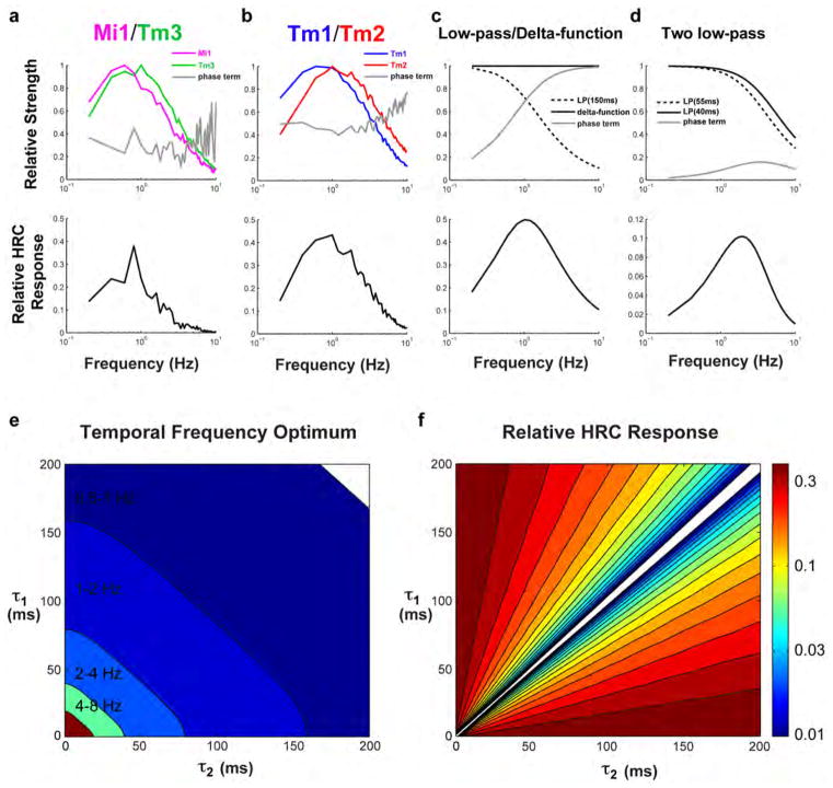
Extended Data Figure 7. Numerical and analytical HRC responses.

a, b, We plot three terms in equation (2) of the Methods, and the total HRC response, using the empirical measurements for Tm1/Tm2 and Mi1/Tm3 as the twoinput arms for the correlator (f₂(t) and f₁(t), respectively). The analytical results computed here match the numerical ones shown in Fig. 4. Here and in all subsequent plots, we normalize the filter values so that they have a maximum of 1, and compute the relative HRC response from those normalized filters and the phase term. c, The same three components of equation (2) are plotted in the special case where f₁(t) =δ(t) and ${\mathrm{f}}_2(\mathrm{t})=\frac{1}{\mathrm{\tau }}{\mathrm{e}}^{-\mathrm{t}/\mathrm{\tau }}$. We plot the result with τ =150 ms, so that the peak response occurs at ~1 Hz. d, The same components of equation (2) are plotted in the case where both f₁(t) and f₂(t) are first-order low-pass filters, with time constants of 40 ms and 55 ms, respectively. e, False-colour plot of the temporal frequency optimum for various combinations of τ₁ and τ₂. Many combinations result in frequency optima near 1 Hz. f, The value of the relative HRC response at the optimal frequency in e is plotted for those same combinations of τ₁ and τ₂. To compute this, temporal filters have a maximum gain of 1, as in a–d. The responses become small primarily when the phase term becomes small. When the phase term is very small, the subtraction performed by the HRC is susceptible to noise, since it can be subtracting two larger numbers to yield the small difference. Therefore, filter combinations with very small differences seem less biologically plausible than those with larger phase terms. The phase terms for the two model HRCs in a and b are between 0.2 and 0.4 in the 1-Hz region, larger than for the toy model shown in d.