A maximum entropy approach to the study of residue-specific backbone angle distributions in α-synuclein, an intrinsically disordered protein

Abstract

α-Synuclein is an intrinsically disordered protein of 140 residues that switches to an α-helical conformation upon binding phospholipid membranes. We characterize its residue-specific backbone structure in free solution with a novel maximum entropy procedure that integrates an extensive set of NMR data. These data include intraresidue and sequential H^N–H^α and H^N–H^N NOEs, values for ³J_HNHα, ¹J_HαCα, ²J_CαN, and ¹J_CαN, as well as chemical shifts of ¹⁵N, ¹³C^α, and ¹³C′ nuclei, which are sensitive to backbone torsion angles. Distributions of these torsion angles were identified that yield best agreement to the experimental data, while using an entropy term to minimize the deviation from statistical distributions seen in a large protein coil library. Results indicate that although at the individual residue level considerable deviations from the coil library distribution are seen, on average the fitted distributions agree fairly well with this library, yielding a moderate population (20–30%) of the PP_II region and a somewhat higher population of the potentially aggregation-prone β region (20–40%) than seen in the database. A generally lower population of the α_R region (10–20%) is found. Analysis of ¹H–¹H NOE data required consideration of the considerable backbone diffusion anisotropy of a disordered protein.

Introduction

The study of the backbone conformational distribution of intrinsically disordered proteins (IDP) has attracted considerable interest in recent years,^1–6 building on extensive prior work that analyzed backbone torsion angle propensities in synthetic peptides.^7–12 The realization that many of the IDPs can form amyloids, which are closely linked to a wide range of diseases, has added impetus to their study.^13,14 α-Synuclein (aS) is a 140-residue IDP, with an N-terminal 100-residue region that is mostly positively charged, and a highly acidic 40-residue C-terminal tail. The N-terminal region binds to negatively charged lipid membranes while adopting an α-helical conformation, whereas the C-terminus remains dynamically highly disordered.^15,16 In free solution, the backbone chemical shifts of the N-terminal region initially were interpreted as indicative of a weak α-helical propensity,¹⁵ but subsequent analysis found this helical population to be rather low.¹⁷ In fact, using refined random coil chemical shift reference values,¹⁸ aS was shown to have chemical shifts that are considerably closer to random coil values than any other IDP studied to date.¹⁹ This means that locally the aS backbone closely resembles a random coil, even though globally the presence of some long-range order is evidenced by compaction of the protein relative to an idealized random coil, as well as by long-range paramagnetic relaxation effects.^20–22 Presumably, this compaction results from weak, nonspecific electrostatic interaction between the protein's oppositely charged N- and C-terminal regions,^23,24 and is rather different in character from the type of compaction observed, for example, in a destabilized triple mutant of the protein Im7, which also exhibits close to random coil chemical shifts.²⁵

A number of increasingly sophisticated methods have been developed to present an ensemble description for this IDP.^22,26,27 Effective programs have also been developed to predict structural propensity from NMR chemical shifts,^17,26,28 but these programs rely on relatively few experimental data and focus on secondary structure, i.e., cooperative formation of structural elements. A combination of the Flexible-Meccano²⁹ and ASTEROIDS³⁰ programs can generate ensembles of random coil structures,²⁷ and has been applied to the study of non-native states of hen lysozyme, using a large number of J couplings and chemical shifts, but no NOE data.³¹ Alternatively, the program Ensemble^32–35 is widely used to select conformers from backbone models generated with the program TraDES.³⁶ A recently established database, pE-DB, for deposition and retrieval of such ensemble models and their underlying restraint reflects the widespread interest in gaining structural insights for IDPs and unfolded states of proteins in general.³⁷ However, although ensemble models of IDPs can be insightful for providing a pictorial view of the backbone conformations sampled by such a protein, it is important to realize that the majority of input parameters commonly used for selecting members from TraDES or Flexible–Meccano ensembles strictly report only on local backbone propensities. For example, homo- and heteronuclear J couplings simply reflect intervening torsion angles, and chemical shifts are dominated by the intraresidue backbone torsion angles, with only a minor effect related to torsion angles in the immediately adjacent residues. Residual dipolar couplings (RDCs), although commonly used as global parameters in well-ordered proteins, primarily report on the “extendedness” of the local backbone in disordered proteins.^38–41 Sources of true long range information can include NOEs, chemical shift perturbation, and paramagnetic relaxation enhancement (PRE). However, long-range NOEs in IDPs often are exceedingly weak and therefore difficult to identify unambiguously, and they only have been used rather infrequently to restrain IDP backbone ensembles.^34,42,43 Chemical shift perturbation (CSP), which reports on small effects of a conservative mutation made at one location in the sequence on chemical shifts of distant residues, can be an exquisitely sensitive method for identifying transient long-range contacts.⁴⁴ However, it lacks a quantitative relation to link the ensemble fraction and distance to the magnitude of the CSP, and therefore is primarily qualitative in nature. Similarly, PRE provides a very sensitive measure for transient long-range contacts in a disordered protein, but analogous to the NOE effect, its quantitative use is complicated by the fact that the PRE is a function not only of distance and population but also of the applicable spectral densities.^45–49 In the present study, we therefore limit ourselves to characterizing only the local backbone torsion angle populations that can be derived from NMR observables, where conformations sampled by a given residue can simply be described in terms of a moderate number of voxel populations in a two-dimensional Ramachandran map, rather than the exponentially larger space sampled by the full protein backbone. As experimental restraints, we use ¹H, ¹³C, and ¹⁵N chemical shifts, four different types of J couplings, and short-range NOEs.

In principle, the aforementioned problem with the unknown spectral densities in IDPs, needed for converting NOEs into distance restraints, can be addressed by integrating the NOE data into a molecular dynamics calculation, which restrains the distances and spectral density terms in the trajectory to be consistent with the NMR data.^43,50 In practice, however, generating trajectories of sufficient length, while minimizing their dependence on the parameterization of the force field used, is not yet computationally tractable with commonly available resources. Therefore, we here introduce an approximate, empirical method for correlating short-range NOE intensities to internuclear distances in IDPs. Molecular dynamics trajectories on a 40-residue fragment of aS quantitatively support the anisotropic rotational diffusion of the protein backbone, which underlies our empirical method for converting ¹H-¹H NOE intensities into internuclear distances.

While in the present study we collected all NMR data on full length aS, only strictly local parameters were measured at high precision. As a consequence, analysis of structural preferences of the protein is restricted to local backbone angle propensities, and not intended to generate ensembles of realistic full chain models. Our analysis is therefore largely analogous to prior investigations of short, disordered peptides, which have been studied in great detail over the past few decades, both by NMR, infrared, and Raman spectroscopies,^{6,10,11,51,52} as well as by SAXS.⁵³ Some of these prior results argue for a high fractional population of polyproline II (PP_II) conformations,^5,54 but other results contradict this conclusion.^6,53 For small peptide fragments of hen lysozyme, conformational propensity was found to depend on peptide length, indicative of a threshold in size needed to switch from random coil to a partially ordered structure.¹⁰ By contrast, for aS we find that chemical shifts of peptide fragments fall very close to those of the full length protein, confirming the close similarity in backbone angles sampled by the full length protein and shorter peptide fragments of it. Our data therefore provide a detailed view of the propensities of the backbone chain in the context of a full length IDP, not impacted by end effects. At the same time, the large number of residues in aS for which detailed NMR measurements were made permits an evaluation of the statistical variation within a given residue type, and between different residues.

With only 10 observables available to define the ensemble of backbone torsion angles sampled by each residue on a ∼100-voxel grid, experimental information is insufficient to uniquely define the angular distributions. However, by using a maximum entropy computational approach, we show that it is readily possible to define residue-specific backbone torsion angle distributions that deviate only moderately from those seen in a statistical coil library, while greatly improving the fit to experimental data over what the library populations would predict.

Results

Most past analyses of unstructured peptides in terms of conformational ensembles aimed at describing the system as a sum of a very limited number of discrete conformers, typically β, PP_II, and α_R, and sometimes also including α_L or turn conformations. Populations extracted, and agreement with NMR data, then depend strongly on the precise backbone torsion angle values chosen for each of these conformers. Here, we aim to describe the peptide as a summation of conformers that span all of the torsion angle space seen in coil library databases. To this extent, we have divided the Ramachandran ϕ/ψ map into a grid of 15° × 15° voxels or cells, and for each cell the coil library⁵⁵ segment containing the residue whose ϕ/ψ angles are closest to the center of the cell is selected as the representative conformer. This procedure is carried out for each residue type, and only cells populated above a threshold (≥3 residues) are retained, while the number of conformers found for each cell in the coil library is stored separately for each residue type. On average, about 100 cells are populated above the threshold for each residue type, and the NMR-related parameters (interproton distances, r_HH, J-values, and chemical shifts) for the residue closest to the center are calculated. In principle, the distribution sampled by any residue in aS then can be determined by assigning weights, w_k (Σ_k w_k = 1), to the cells such that the sum over the calculated NMR-parameters optimally matches the experimental data. The calculated NMR weight-averaged observable, I_calc (q), for any given residue in the sequence is then given by:

(1)

where I_k(q) is the value calculated for cell k, and q indicates the type of observable. N_c is the number of populated cells. The normalized residual in the total fit, averaged over all N_q = 10 restraint types, for any given residue is defined by:

(2)

where σ(q) is the estimated uncertainty in I_exp(q) (SI Text). In practice, minimizing χ² is an ill-determined problem as there are N_c ≈ 100 weights to be defined by 10 observations per residue. Therefore, it is desirable to regularize the weight calculations, and to search for the distribution of conformers that tries to follow the natural distribution found in the coil library as close as possible while also satisfying the experimental data. For this purpose we use the principle of maximum entropy, as described below.

As experimental restraints, we use the backbone ¹³C^α, ¹³C′, and ¹⁵N chemical shifts, four different types of J couplings, and intraresidue and sequential NOEs. Incorporation of chemical shift terms into Eq. (2) is closely analogous to procedures followed by others,^31,34,56,57 and is briefly summarized in the Materials and Methods section. Inclusion of the ³J_HNHα, ¹J_HαCα, ²J_CαN, and ¹J_CαN coupling information is also analogous to earlier work, but with some adaptations discussed below. Analysis of NOEs to derive local structural information in IDPs has only been used sparingly, in part because such NOEs tend to be relatively weak, but also because the anisotropy of the IDP chain motion makes it inappropriate to simply assign a uniform, isotropic rotational correlation time to the system. In principle, it is possible to use such NOEs to restrain a dynamics trajectory that encodes both interproton distances as well as the applicable spectral density terms,^42,50 but in practice this proved impossible for a system as large as aS. In this work, we introduce an alternative approach to derive applicable spectral density terms, based on analysis of ¹⁵N relaxation rates, while using an empirical orientational dependence of the interproton vector relative to the C^α–C^α chain direction to account for diffusion anisotropy of the chain. As discussed below, the latter is supported by unrestrained dynamics calculations on a long fragment of aS in a bath of explicit water.

Ramachandran Grid Populations Using Experimental Data and Maximum Entropy

To prevent overfitting of the experimental data while determining the populations of Ramachandran map voxels sampled by any given residue, we use the maximum entropy criterion. Implementation is in full analogy to its recent use for identifying ensembles that best agree with SAXS data.⁵⁸ The entropy term is defined by:

(3)

where is the reference weight for the conformer k, derived from the population of cell k in the coil library. In an effective free energy function,

(4)

the parameter θ then controls the entropy impact on the effective energy, χ². The free energy function G is minimized by means of a simulated annealing algorithm.⁵⁸ Use of a high θ-value (e.g., θ = 50) results in a distribution that closely follows the coil library distribution, whereas a small value (e.g., θ = 0.1) can result in overfitting and poor convergence, with sometimes high populations of cells that fall close to the edges of the allowed region in the Ramachandran map.

The optimal value of θ varies somewhat from residue to residue, and can be selected by plotting χ² as a function of S [Fig. 1(a)]. When repeating calculations for increasing values of θ, the value that shows a modest increase (the larger of 0.25 or 25% of the χ² value obtained for θ = 0.4) is selected to define the ensemble that best describes the experimental data [Fig. 1(b)].

Figure 1.

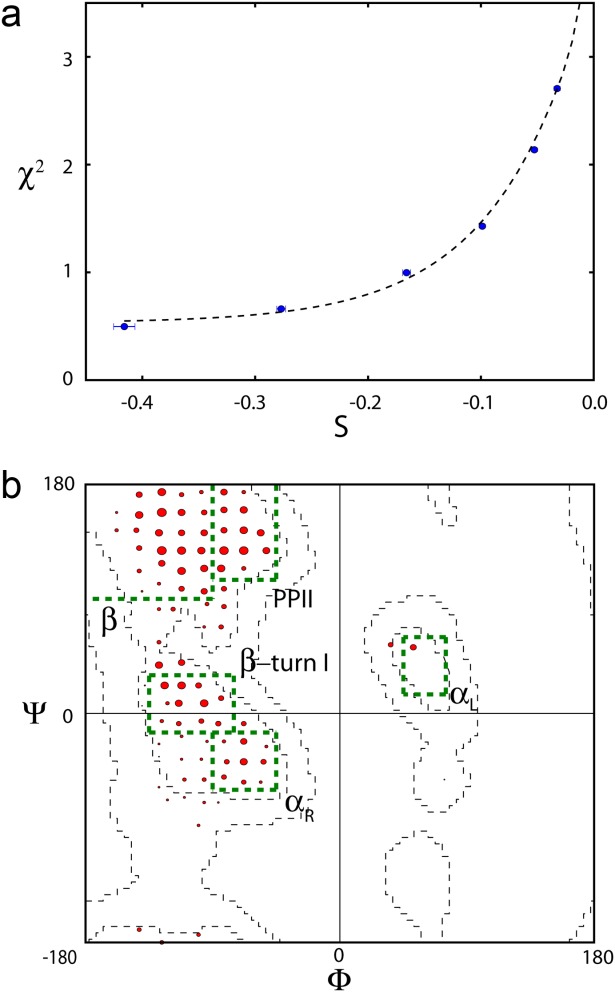
Example of distribution fitting of a residue's backbone angles to 10 independent experimental NMR parameters, shown for V40. (a) Plot of χ² versus S, for calculations carried out at θ values of 0.4, 0.8, 1.6, 3, 6, and 10 (left to right). S = 0 corresponds to a ϕ/ψ distribution that matches that of the coil database. (b) Backbone conformational distribution at θ = 0.8. The population of each conformer is proportional to the area of the corresponding red circle. Green boxes mark secondary structure regions, β, PP_II, type I β-turn, α_R, and α_L. Results shown in both panels represent averages over eight simulated annealing runs. Conformer populations for all nonGly/Pro residues with complete sets of 10 NMR parameters are shown in Supporting Information Figure 2.

J couplings for restraining ϕ/ψ space

Structural parameters that can be measured at high accuracy for aS include the ³J_HNHα, ¹J_CαHα, ¹J_CαN, and ²J_CαN values. The ³J_HNHα values in an IDP were previously measured at very high precision (<0.05 Hz)¹⁹ and were shown to be quite insensitive to residue type, H-bonding effects, and structural variables other than ϕ, as evidenced by an RMSD of about 0.4 Hz between experimental values and those predicted by a Karplus curve when using an RDC-refined high resolution X-ray structure.^{59,60 1}J_CαHα couplings are sensitive to both ϕ and ψ, and residue-specific random coil values were reported previously.^{61 1}J_CαHα ranges from ∼134 Hz in the α_L region to ∼148 Hz for α_R.⁶²

¹J_CαN and ²J_CαN also have a Karplus-like dependence on ψ.^10,63 Although their values vary by less than about 3 Hz across the entire range of ψ angles, they can be measured at very high precision^63,64 and have proven to be useful for characterizing structures of disordered peptides and proteins.^10,31 For ¹J_NCα, the Karplus equation parameterization of Wirmer and Schwalbe was used.^63,65 For ²J_NCα, the Karplus equation parameterization of Ding and Gronenborn is commonly used.⁶³ However, we noticed a small but systematic residue-dependent offset between observed and best-fitted ²J_NCα data when generating ensembles of conformers that aimed to simultaneously fit all 10 NMR observables (4 types of J couplings, 3 chemical shifts, and 3 NOEs). The problem was most apparent for the β-branched Val, Ile, and Thr residues, as well as Ser. Evaluation of ²J_NCα values reported by Schmidt et al.⁶⁶ for a set of proteins of known structure confirms the presence of a small systematic difference between these four residue types versus all others (Fig. 2). We therefore used a slightly amended ²J_NCα Karplus equation:

Figure 2.

Plot of ²J_NCα values, previously reported by Schmidt et al.⁶⁶ for a set of six proteins of known structure, supplemented by values measured by us for protein GB3 (unpublished data), against the intervening torsion angle ψ, taken from the corresponding high resolution X-ray structure. Values are shown only for residues with backbone chemical shift values that are consistent with the X-ray structure, as judged by the program TALOS-N.⁶⁷ Red symbols correspond to Val, Ile, Thr, and Ser residues. Blue symbols are shown for all other residues. The solid line corresponds to ²J_NCa = 8.15 − 1.51 cos(ψ) − 0.66 cos²(ψ) Hz, where ψ is the torsion angle of the residue on which ¹³C^α resides.

(5)

where C = 7.65 for Val, Ile, Thr, and Ser, and C = 8.15 for the remaining residues.

Chemical shifts for restraining ϕ/ψ space

Backbone ¹³C and ¹⁵N chemical shifts depend on both ϕ and ψ, and here we use the empirically determined (ϕ,ψ)-dependence⁶⁸ of backbone ¹⁵N, ¹³C′, and ¹³C^α shifts as additional restraints (Material and Methods section). ¹H chemical shifts, which show a weaker (ϕ,ψ)-dependence than ¹⁵N and ¹³C and can be substantially impacted by ring current effects, were not included in our analysis. Experimental chemical shifts used in the present study were taken from Maltsev et al.¹⁹

Backbone dynamics from ¹⁵N relaxation

The backbone dynamics of aS in the absence of lipids has been evaluated previously,^69,70 but was repeated in our study to take advantage of gains in NMR sensitivity and resolution made over the past decade, and to probe the potential presence of conformational exchange contributions to the transverse relaxation rates. The ¹⁵N relaxation data (Supporting Information Table I), recorded at 500 and 900 MHz ¹H frequency, permit mapping of the spectral densities and now show a smoother profile (Fig. 3), but the previously identified increased mobility for the fibril-implicated NAC region⁶⁹ remains evident in decreased ¹⁵N-{¹H} NOE and ¹⁵N R₂ rates (Supporting Information Table II). Comparison of the ¹⁵N R₂ rates recorded at 11.7 and 23 Tesla shows no evidence for any slow or intermediate exchange contributions, confirming that the J(0) spectral densities extracted from the relaxation rates by reduced spectral density mapping⁷¹ are not contaminated by exchange effects. Remarkably, even though the high frequency (50 and 435 MHz) spectral densities are quite homogeneous across the entire sequence, J(0) values vary by more than a factor of two? The lowest J(0) values are found in the NAC region, with highest values for residues in, and immediately following the Pro¹¹⁷-Val-Asp-Pro region in the acidic C-terminal tail. Below, these J(0) values will be used for extracting distance information from the ¹H–¹H NOE data.

Figure 3.

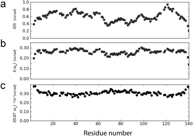
Spectral densities for backbone amide ¹⁵N–¹H pairs in aS at 500 MHz, 15°C, obtained from reduced spectral density mapping of the relaxation rates listed in Supporting Information Table II. (a) J(0), (b) J(ω_N), and (c) J(0.87ω_H), for ω_N = 50.6 × 2π rad/s and ω_H = 499.5 × 2π rad/s. The spectral density values are also listed in Supporting Information Table III.

Measurement of ¹H–¹H NOE data

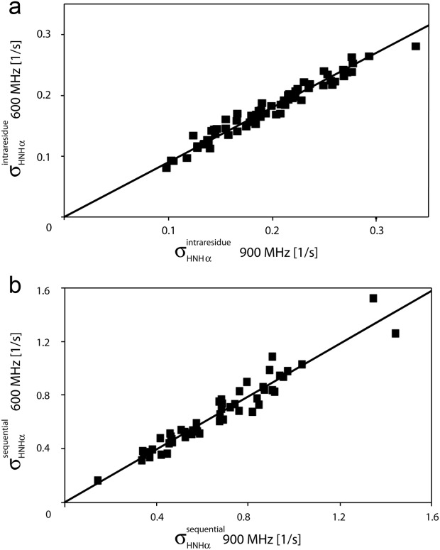
Even though J(0) values in IDPs are small relative to those of a globular protein the same size, an extensive set of intraresidue and sequential NOEs is readily observed for aS (Fig. 4). The intraresidue H^N–H^α distance solely depends on the backbone angle ϕ and varies little (2.9 ± 0.15 Å) in the most-populated, negative ϕ region of the Ramachandran map. ¹H–¹H NOE cross relaxation rates are proportional to the {J(0) – 6J(2ω_H)} spectral density difference.⁷³ Consequently, the corresponding NOEs are found to correlate closely with this term, which was derived independently from ¹⁵N NMR relaxation (Fig. 5). H^N–H^α crossrelaxation rates measured at 600 and 900 MHz are very similar to one another, indicating that the impact of the J(2ω_H) term is negligible for the sequential H^α–H^N NOE [Fig. 6(b)]. However, the intraresidue H^N–H^α NOE is about 10% weaker at 600 MHz as compared to 900 MHz [Fig. 6(a)], pointing to a small contribution of the 6J(2ω_H) spectral density term. However, even at 500 MHz ¹H frequency, the term J(0.87ω_H) is already more than ∼15-fold smaller than J(0) (Fig. 3), and J(0.87ω_H) rapidly decreases with increasing magnetic field strength. Therefore, at 900 MHz, the 6J(2ω_H) term becomes much smaller than J(0) and may be safely ignored. However, as discussed below, anisotropy of the overall chain dynamics and its internal motion potentially complicate the NOE analysis. In particular, the so-called γ-motions,⁷⁴ which correspond to peptide plane oscillations around the – chain direction, are expected to dominate the internal dynamics. Motions that correspond to sampling of backbone torsion angles in the β and PPII regions of Ramachandran space lack distinct energy barriers and are expected to be diffusion-limited in their rates, and to be of comparable amplitudes along the chain. Indeed, as can be seen from Figure 3(c), and also from inspection of J(0.87ω_H) at 900 MHz ¹H frequency (Supporting Information Table III), these high frequency spectral density terms show remarkably little residue-by-residue variation along the protein chain, pointing to quite homogeneous amplitudes and time scales of these γ-motions.

Figure 4.

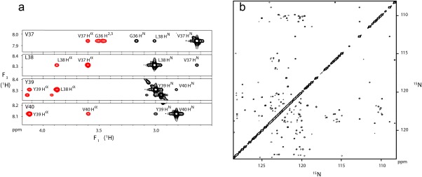
Examples of NOESY spectral data (100 ms NOE mixing; 15°C) recorded for aS. (a) Small regions of strips taken from the 900 MHz 3D ¹H–¹⁵N–¹H NOESY-HSQC spectrum. To achieve improved digital resolution, a narrow F₁ spectral window (5.3 ppm) was used, resulting in aliasing and opposite signs of the amide signals (black contours) relative to the aliphatic signals (red). (b) Partial projection of the ¹⁵N–¹⁵N–¹H 3D NOESY spectrum⁷² of aS (800 MHz) on the ¹⁵N–¹⁵N (F₁, F₂) plane, displaying H^N–H^N NOEs. The projection extends from 8.15 to 8.61 ppm in the ¹H dimension.

Figure 5.

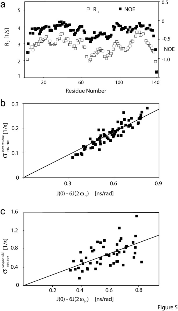
Variation in backbone dynamics of aS, reflected in substantial variations in (a) ¹⁵N transverse relaxation rates, R₂ (open symbols), and ¹⁵N–{¹H} NOE values (both at 500 MHz), and in the wide range of (b) intraresidue H^N–H^α cross relaxation rates, σ_HN–Hα (at 900 MHz), which closely correlate with the spectral densities derived from ¹⁵N-relaxation and (c) sequential H^α–H^N cross relaxation rates, which also scale with ¹⁵N-relaxation derived spectral densities. Considerable scatter in (c) is indicative of residue-by-residue variation in the interproton distance distribution. Sample conditions: 0.2 mM ¹⁵N-enriched aS; pH 6, 20 mM sodium phosphate, 288 K.

Figure 6.

Correlation plot for the (a) intraresidue– and (b) sequential– crossrelaxation rates measured at 600 and 900 MHz ¹H frequency. For (b), which involves short interproton distances when the vector is approximately parallel to the– vector, the slope equals 0.99, indicating that the impact of the 6J(2ω_H) term is negligible, considering that J(2ω_H) is estimated to be about two-fold smaller at 900 MHz compared to 600 MHz ¹H frequency. For the intraresidue– interaction, which makes a large angle with the − vector, the slope is ∼0.9, indicating that the 6J(2ω_H) term is small (∼10% of J(0)).

In contrast to the intraresidue H^N–H^α NOEs, sequential H^α–H^N NOEs show a considerable range of variation superimposed on the correlation with J(0) – 6J(2ω_H) [Fig. 5(c)]. In folded proteins, the sequential H^α–H^N distances exhibit a much larger spread than the intraresidue H^N–H^α pairs. The large variation in sequential H^α–H^N NOEs observed for residues of any given J(0) – 6J(2ω_H) value therefore indicates that they are significantly impacted by residue-by-residue variations in applicable distance distributions, i.e., by conformational propensities.

If motions of dipeptide units in an IDP were isotropic, it would be straightforward to extract the <r_HH⁻⁶> term applicable for the sequential H^α–H^N NOE from the ratio of the sequential and intraresidue H^N–H^α NOE, using the approximately invariant intraresidue H^N–H^α distance as an internal reference. Indeed, in folded proteins the ratio of the sequential and intraresidue H^α–H^N NOE intensities, d_αN(i − 1,i)/d_αN(i,i), is a sensitive measure for the ψ angle of residue i − 1.⁷⁵ However, such an analysis assumes the same spectral densities to be applicable for the intraresidue and sequential H^α–H^N interaction, an assumption that is not compatible with the very high values of the d_αN(i − 1, i)/d_αN(i,i) ratios, in the 3–6 range, typically observed in IDPs.

The J(0) term, which dominates the ¹H–¹H NOE, is expected to depend strongly on the orientation of the ¹H–¹H vector relative to the chain direction. This anisotropy is impacted both by the shape of an extended chain, which even for short peptides results in distinct rotational diffusion anisotropy,⁷⁶ as well as by the differential sensitivity to internal motions, in particular the above noted γ-motions. In the absence of a detailed motional model of the polypeptide chain of an IDP, we here introduce an ad hoc functional form for the angular dependence of the J(0) term applicable for the sequential NOE:

(6)

where J(0)_exp corresponds to the J(0) spectral density derived from ¹⁵N relaxation, and ψ is the backbone torsion angle of residue i. Equation (6) corresponds to an about 2.5-fold anisotropy, with the highest J(0) value for extended conformers (ψ ≈ 120°) and near J(0)_exp values for ψ ≈ −60°. Spectral densities for the intraresidue– and sequential– vectors, which are at relatively large angles from the– vector, are approximated by J(0)_exp, the experimental J(0) spectral density derived for ¹⁵N_i–¹H_i pairs that to a first approximation are orthogonal to–. Below, we demonstrate by evaluation of extended molecular dynamics trajectories of a polypeptide fragment of aS, that Eq. (1) provides a reasonable first order approximation for the impact of J(0) anisotropy on the ¹H–¹H NOE buildup rates.

Dynamic corrections to ¹H–¹H NOEs in a random coil

Long (ca. 1 µs) molecular dynamics trajectories were generated in explicit water for a peptide fragment comprising the 40 N-terminal residues of aS, at three temperatures. Spectral densities were derived from these trajectories as detailed in the Material and Methods section. In Figure 7, we first compare the full spectral density J(0) of sequential H^α–H^N dipole-dipole couplings, including both distance and angular fluctuations, to the spectral density J_a(0) arising from angular relaxation alone. We find that the dynamic contribution to the full spectral density J(0) is determined almost entirely by the rotational motion, J(0) ≈ J_a(0), at all temperatures. The reason is that the distance relaxations C_r(t) of sequential H^α–H^N vectors are dominated by motions that are at least an order of magnitude slower than the angular motions in the MD simulations.

Figure 7.

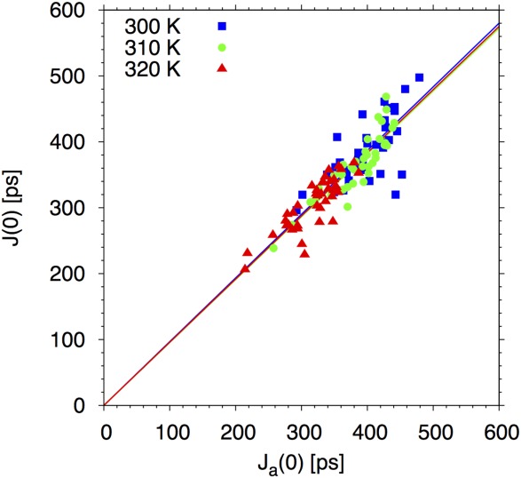
Scatter plot of the MD-derived total spectral density J(0) (y-axis) and of the spectral density J_a(0) for angular motion alone (x-axis) for sequential H^α–H^N couplings. The symbols show results for the individual residues at each of the three simulation temperatures (blue squares: 300 K; green circles: 310 K; red triangles: 320 K). The lines show least-squares straight-line fits of the form J(0) = cJ_a(0) for each of the temperatures. The average slope of c = 0.96 ± 0.01 (with the error determined by the bootstrap method) indicates that rotational dynamics dominates the relaxation.

For computational purposes, we define the dynamic correction to the ratio of spectral densities of sequential and intraresidue H^α–H^N NOEs, normalized by the respective static <r⁻⁶> averages, as:

(7)

Figure 8 shows a scatter plot of this ratio, calculated for sequential (–) and intraresidue interactions (–) of each residue i for three temperatures, as a function of the weighted population w_i in the extended state evaluated along the simulation trajectory of duration T:

Figure 8.

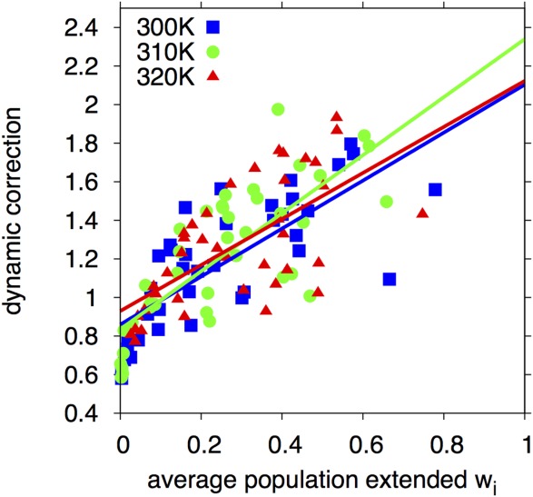
Dynamic correction [Eq. (7)] to J(0) for sequential H^α–H^N couplings as a function of the weighted population [Eq. (8)] in the extended configuration. Results are shown for each residue at three temperatures (blue squares: 300 K; green circles: 310 K; red triangles: 320 K). The lines show least-squares straight-line fits for each of the temperatures. The ratio of the factors extrapolated to weights of 1 and 0 are 2.45, 2.80, and 2.28 at T = 300, 310, and 320 K, respectively. A global fit of all data gives a ratio of 2.51 ± 0.20, with the error determined by the bootstrap method. The simulation estimates for the correction are therefore fully consistent with the functional form of Eq. (6) and the maximum magnitude of 2.5 for the correction factor used in the analysis of the experimental NOE data.

(8)

This is the same weight function used to correct the experimental J(0) [Eq. (6)]. With the two nonoverlapping exponentials accounting for periodicity, w_i is effectively bounded between 0 and 1. As can be seen from Figure 8, the correction increases approximately linearly with the weight w_i at all three temperatures. The ratio of the corrections extrapolated to w_i = 1 and w_i = 0 equals about 2.5, fully consistent with the correction used for the experimental J(0) values [cf Eq. (6)]. The reason why this correction can be extracted directly from the simulation trajectories is that the conformational dynamics associated with radial motions is slow as compared to angular motions, as discussed above. As a result of this time-scale separation, the correlation functions C(t) (Material and Methods section) and thus, by definition, J(0) are well approximated by weighted population averages.

Evaluation of residue-specific ϕ/ψ distributions

For aS, complete sets of all 10 aforementioned parameters (³J_HNHα, ¹J_CαHα, ¹J_CαN and ²J_CαN, δ_15N, δ_13Cα, δ_13Cβ, d_αN (i, i + 1), d_αN(i,i), and d_ΝN(i,I + 1)) were obtained for 52 residues, not including 18 Gly and 5 Pro residues. Using Eqs. (2) and (4), and the σ-values defined in the Experimental Section, these values were used to derive lowest free energy ϕ/ψ distributions by means of a simulated annealing protocol, while weakly restraining these distributions to not deviate radically from those seen in the coil database. The weight, θ, used to conform with the statistical database, and implemented through the principle of maximum entropy [cf. Eq. (4)], was varied by approximately doubling θ in successive simulated annealing runs. The distribution that shows a modest increase in total χ² when doubling θ (the larger of 0.25 or 25% of the χ² value obtained for θ = 0.4) is selected as representative of the ensemble that best describes the experimental data. For most residues, θ = 0.4 or 0.8 yielded optimal results, and fits to the experimental data that for many residues were one to two orders of magnitude better than obtained for coil populations of Ramachandran space (Fig. 9). On the other hand, coil database ϕ/ψ distributions were approximately compatible with experimental data for several residues too, incl. A19, K21, and T92. Distributions of ϕ/ψ for all 52 residues, analogous to those shown in Figure 1(b), are included in the Supporting Information.

Figure 9.

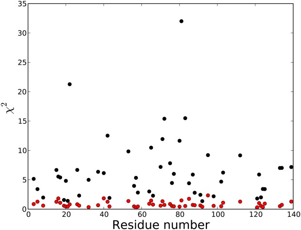
χ² as a function of residue number, obtained when using the coil database populations of conformers to predict the experimentally observed parameters (black symbols) and when using the optimized populations of Supporting Information Figure 2 (red).

Discussion

To compare our results with prior studies of peptides, we group our cells into five regions, β, α_R, PP_II, type I β-turn, and α_L [Fig. 1(b)]. For nearly all residues, the PP_II population falls in the 20–30% range, closely following the statistical coil populations (white bars in Fig. 10), but the β-region is more highly populated in our aS results than in the database for Ala, Asp, Asn, Gln, Glu, Lys, and Thr residues. The small standard deviations seen in Figure 10 indicate that residues of a given type tend to yield similar results (Supporting Information Fig. 3), while in a number of cases deviating significantly from the populations seen in the statistical coil library. Population of the α_R region, on average, is lower than seen in the coil library, in agreement with what was found in many of the peptide studies.^7–11 Our results indicate that the type I β-turn region is somewhat less populated than seen in the coil library, but its 10–20% population is nevertheless significant. Neither chemical shifts nor J couplings yield a unique signature for this region, but the short distances between sequential H^N atoms (2.1–2.4 Å) give rise to substantial amide–amide NOEs, permitting unambiguous identification of their presence. The only other region with short H^N–H^N distances is α_R (∼2.8 Å), and a very high population would be required to satisfy the experimentally observed NOE intensity, incompatible with the other observed NMR parameters. In contrast to the type 1 β-turns reported recently in Tau protein,⁷⁷ another IDP, in aS the propensity for this turn type is relatively flat across the protein sequence. Analogous to the coil library, our data show no evidence for significant population of the α_L region, which carries as its most distinct NMR features a very small ¹J_HαCα and a strong intraresidue H^N–H^α NOE. Even Asn residues, which show an elevated α_L presence in the coil library (∼15%), exhibit low α_L occupancy (5%) in aS. The latter observation also highlights that our results are not unduly biased by the entropy term, which skews our populations towards those of the coil library.

Figure 10.

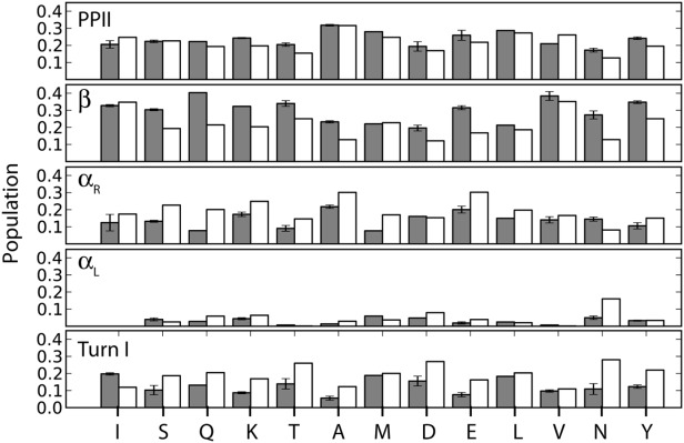
Average populations of the five regions marked in Figure 3(b): β, PP_II, type I β-turn, α_R, and α_L, by residue type as observed in aS (gray bars), with the corresponding population in the coil library of Fitzkee et al.⁵⁵ shown in white. Residue-specific values are presented in Supporting Information Fig. S3.

However, our analysis also shows that, on a courser scale, the distribution of backbone torsion angles in aS does not differ drastically from that seen in the statistical coil library obtained from X-ray structures. For nearly one-third of the residues, a reasonable fit (χ² ≤ 3) to the experimental data (Fig. 9) is obtained when using the ϕ/ψ distribution seen in the coil library. The absence of a dominant PP_II population is clearly evidenced by our results, even for Ala17, Ala19, and Ala91, which are part of stretches of three consecutive Ala residues with complete NMR data. On the other hand, our results also indicate that some deviations from coil library populations are present in aS (Fig. 10, Supporting Information Fig. 3) with, on average, the β-region being populated somewhat higher than in the coil library, an effect most pronounced for residues in the fibril-implicated NAC region (residues 61–95). The variation in backbone dynamics along the sequence is quite pronounced, and considerably larger than seen, for example, in fully denatured ubiquitin.⁷⁸ In particular, the low J(0) spectral density observed for the NAC region shows it to be considerably more flexible than the remainder of aS (Fig. 3A).

Material and Methods

NMR experiments

3D ¹H–¹⁵N–¹H NOESY-HSQC and ¹⁵N–¹⁵N–¹H HSQC-NOESY-HSQC spectra were recorded with a mixing time of 100 ms at 15°C on a Bruker AV-III 900 MHz spectrometer equipped with a single axis gradient TCI cryogenic probe. The sample contained 0.35 mM ¹⁵N-enriched aS and 20 mM sodium phosphate at pH 6. The two spectra consisted of 1024* (F₃, ¹H, 94.7 ms) × 120* (F₂, ¹⁵N, 62.2 ms) × 230* (F₁, ¹H, 52.7 ms) and 1024* (F₃, ¹H, 94.7 ms) × 126* (F₂, ¹⁵N, 64.5 ms) × 126* (F₁, ¹⁵N, 64.5 ms) complex data points, respectively. After the NOE mixing period, a sensitivity-enhanced, gradient-selected HSQC was employed.⁷⁹ To maximize digital resolution, a small spectral width of 4.84 ppm in F₁ was used in the ¹H–¹⁵N–¹H NOESY-HSQC experiment (resulting in aliasing and opposite phases of the amide resonances) and both spectra were recorded using two scans per FID and a two-step phase cycling scheme. In the ¹H–¹⁵N–¹H experiment, the ¹H 90° pulses before and after t₁ evolution were phase cycled to yield States-TPPI quadrature detection, and a two-step phase cycling was applied to the ¹⁵N 90° pulse prior to t₂, in addition to quadrature detection by gradient-enhanced coherence selection,⁷⁹ thereby better canceling the residual solvent signal. The absence of a phase cycle for axial peak suppression in the F₁ dimension resulted in a strong peak at the edge of the indirect ¹H dimension (F₁). However, the narrow spectral width was chosen such that the axial artifact, largely removed during the data processing, did not interfere with the cross peaks or folded amide diagonal. Similarly, the first ¹⁵N 90° pulse in the first HSQC segment of the ¹⁵N–¹⁵N–¹H HSQC-NOESY-HSQC experiments, was alternated in successive scans, to also yield a two-step phase cycle. 3D NOESY spectra with similar digital resolution and acquisition parameters were also recorded on Bruker AV-II 600 MHz and AV-III 800 MHz spectrometers, both equipped with a cryogenic probe. The NOESY data collected at multiple magnetic fields allowed us to estimate the relative contribution to the NOE intensities of the field-dependent J(2ω_H) term relative to J(0), but only the better resolved and most accurate 900 MHz data were used as input restraints for conformer selection by the simulated annealing protocol.

Longitudinal ¹⁵N R₁ relaxation rates and steady-state heteronuclear ¹⁵N–{¹H} NOE at 15°C were measured at 900 MHz, using methods described by Lakomek et al.⁸⁰ The sample contained 0.15 mM perdeuterated ¹⁵N-enriched aS and 20 mM sodium phosphate at pH 6. For the R₁ and ¹⁵N–{¹H} NOE measurements at 900 MHz, the TROSY readout was used.⁸⁰ Six 2D experiments were interleaved, with variable T₁ delays of 0, 200, 400, 600, 800, and 1000 ms, each consisting of 2048* (F₂, ¹H, 206.5 ms) × 256* (F₁, ¹⁵N, 116.7 ms) complex data points. Using an interscan delay of 1.5 s and 8 scans per FID, the total data recording time was 13 h. For the NOE measurement, two experiments with and without the proton saturation pulse train were interleaved, each consisting of 2048* (F₂, ¹H, 206.5 ms) × 310* (F₁, ¹⁵N, 141.4 ms) complex data points. In the NOE experiment, after the initial ¹⁵N 90° pulse for removing the so-called BEST TROSY effect,⁸¹ the water was first presaturated using an RF field strength of 89 Hz for 1 s, followed by a train of nonselective 180° ¹H pulses centered on the amide proton resonances for 7 s, while a total delay of 8 s was used in the reference experiment. The total data collection time was 34 h using 12 scans per FID.

R₁ and ¹⁵N–{¹H} NOE were also measured on a Bruker AV-III 500 MHz spectrometer with a cryoprobe using the same sample, methods, and comparable acquisition parameters as described above. In addition, transverse ¹⁵N R₂ relaxation times were determined at 500 MHz ¹H frequency using a R_1ρ experiment⁸⁰ with a spin lock RF power of 1.4 kHz. Six interleaved 2D spectra with spin lock durations of 10, 20, 80, 160, 270, and 380 ms were recorded, each consisting of 1536* (F₂, ¹H, 219.6 ms) × 220* (F₁, ¹⁵N, 180.4 ms) complex data points. A long interscan delay of 5 s was used to reduce the amplifier duty cycle and RF heating effects. With 8 scans per FID, the total data recording time was 35 h. The ¹⁵N carrier was positioned at 118 ppm, and the R₂ rates were corrected for the off-resonance tilted field, using the relation R₂ = R_1ρ/sin²θ – R₁/tan²θ with tan θ = ω₁/Ω, where R_1ρ is the directly measured decay rate of the R_1ρ experiment, ω₁ is the spin-lock RF field strength and Ω the offset from the ¹⁵N carrier.

The measurement of the ³J_HNHα couplings at 900 MHz and 15°C has been described previously.¹⁹ The ²J_CαN couplings were determined from a 2D high resolution TROSY spectrum without the ¹³C^α decoupling pulse but with a selective ¹³C′ and an IBURP ¹³C^β decoupling pulse (covering a bandwidth from 35 to 15 ppm), applied in the indirect ¹⁵N dimension. The spectrum was recorded on a Bruker AV III 800 MHz spectrometer at 15°C using a sample of 0.34 mM perdeuterated and ¹³C/¹⁵N-enriched aS, with acquisition times of 213 (¹H, t₂) and 1064 (¹⁵N, t₁) ms (2048* × 2048* data matrix). Using an interscan delay of 1.2 s and 16 scans per FID, the measurement time was 36.5 h. At this digital resolution, the couplings of ¹⁵N to both the intraresidue and preceding ¹³C_α were well resolved for nearly all cross peaks, resulting in a doublet of doublet splitting pattern from which two measurements of ²J_CαN and ¹J_CαN were made for each amide, and the averaged value is used and reported in this study.

The ¹J_CαHα couplings were measured from the doublet splitting in the ¹³C dimension of a 3D TROSY-HN(CO)CA spectrum, recorded without application of the ¹H^α decoupling pulse during the 28 ms constant-time ¹³C evolution period, which effectively eliminates the ¹J_CαCβ splitting for improved spectral resolution. The 3D data matrix consisted of 700* × 30* × 86* complex points for acquisition times of 97.1, 195, and 28 ms in the ¹H, ¹⁵N, and ¹³C dimensions, respectively. Note that the ¹⁵N dimension was recorded using 30 complex data points only, but with a narrow spectral window of 2.53 ppm to achieve high digital resolution. The ¹⁵N acquisition time of 195 ms, much longer than the ¹J_NCO refocusing delay of ∼25 ms, was realized by using the mixed-time (MT) evolution approach.⁸² The total data recording time was 35 h, using a 1 s interscan delay and 8 scans per FID.

All the NMR data were processed using the NMRPipe software⁸³ and analyzed in NMRDraw and Sparky.⁸⁴

Selection of conformers from the coil library

The coil library used in our study was originally compiled by Fitzkee et al.⁵⁵ and represents a database of fragments of protein X-ray structures that do not adopt regular α-helical or β-strand secondary structure. From this full coil library, available on-line, we selected fragments using the following criteria:

• sequence identity between fragments ≤20%,

• resolution of the X-ray structure is 1.6 Å or better,

• refinement factor, R, of the X-ray structure ≤0.25.

Fragments were selected from 2093 different protein chains. Selected fragments have been additionally filtered: Only fragments with a length of the coiled region of three or more amino acids were retained. To exclude any influence of adjacent fragments with secondary structure on the distribution, we further excluded the most N- and C-terminal residue for each selected coiled fragment. The number of residues for each type remaining after these procedures were applied is listed in Supporting Information Table IV.

The populations of each of the Ramachandran map voxels that optimally fit the experimental data while minimizing the effective free energy function of Eq. (4) were determined by using a simulated annealing protocol.⁵⁸ For each value of θ, and for each residue, the procedure was repeated 5 times, using different random seeds. Calculations were performed on a workstation with two 6-core Intel 2.67 GHz Xeon X5650 processors, using 12 MB of Cache memory per processor, 12 GB of DDR3-1333 ECC-registered memory, and using Hyper-threading. On average, 10,000 steps of simulated annealing minimization took 63 min per residue using one thread.

The minimum size of the voxels used, 15° × 15° was determined by two factors: First, the statistical coil library approach used in our study requires significant population of each voxel in order to remove the impact of statistical fluctuations of the database voxel population, when using the entropy factor to deviate minimally from the database distribution. Second, convergence of the simulated annealing protocol rapidly decreases when using voxel sizes significantly smaller than 15° × 15°.

Calculation of synthetic NMR parameters for the database structures

Calculation of the J-coupling constants was carried out using Karplus-type equations, using the torsion angles taken from the database. ¹J_CαHα values were calculated using the parameterization of Vuister et al.⁶¹ with residue-type specific random coil values. The random coil value of Ala was decreased by 1.7 to 142 Hz, as both DFT calculations and our experimental results were not compatible with this value being much higher than that of other residues. For ³J_HNHα the Karplus parameterization of Vogeli et al. was used using the ‘rigid model’ parameterization. For the small protein GB3, these parameters yielded an RMSD of 0.42 Hz between observed and calculated ³J_HNHα values.⁵⁹ Following subsequent RDC refinement of the H^N positions,⁸⁵ this RMSD decreased to 0.34 Hz. Considering that this RMSD includes the effect of residual uncertainty in ϕ, measurement error in ³J_HNHα, and potential impact of H-bonding, residue type, and conformational effects other than the ϕ torsion angle, the impact of these last three factors must be considerably less than 0.34 Hz. For ¹J_NCα, the Karplus equation parameterization of Wirmer and Schwalbe was used.^63,65 For ²J_NCα, the Karplus equation parameterization of Ding and Gronenborn was used,⁶³ but the value of the constant factor (7.85 Hz) was increased by 0.3 to 8.15 Hz for all residues except Ser and the β-branched Val, Ile, and Thr residues, for which the value was decreased to 7.65 Hz. Without this adjustment, small systematic discrepancies between our experimental values and those resulting from the simulated annealing search remain. Evaluation of ²J_NCα values reported by Schmidt et al.⁶⁶ for a set of proteins of known structure confirmed the presence of this small systematic difference between these two pools of residues.

Prediction of the chemical shifts was carried out using random coil chemical shifts and neighboring residue corrections taken from the program SPARTA.⁶⁸ Residue-specific ϕ/ψ-dependence of the secondary chemical shift was extracted from the SPARTA+ database,⁸⁶ and the predicted chemical shift was calculated as the sum of the random coil chemical shift, the secondary chemical shift, and the correction for neighboring residues.

The cross relaxation rates for the aS ensemble were calculated from the weighted average of the rates calculated for the corresponding grid points. For each grid point, the ¹H-¹H cross relaxation rate at 900 MHz was calculated using the equation:

(9)

where r_HH is the interproton distance, J(0) the spectral density at zero frequency, D = hµ₀γ_H²/(16π²) with µ₀ being the permeability of vacuum, γ_H the proton gyromagnetic ratio and h being Planck's constant. We neglected the impact of the 6J(2ω_H) term because this term is very small compared to J(0) (Supporting Information Table SIII). The term J(2ω_H) at 600 MHz ¹H frequency is estimated by propagation from the J(0.87*900*10⁶*2π) value determined from reduced spectral density mapping.⁷¹

Weighting of constraints

For calculating the χ² value [Eq. (2) main text] the following error values σ(q) were used:

Chemical shifts [ppm]: ¹⁵N 1.28; ¹³C′ 0.4; ¹³C^α 0.4.

J couplings [Hz]: ¹J_CαHα 0.35; ²J_CαN 0.2; ¹J_CαN 0.2; ³J_HNHα 0.15.

¹H–¹H cross relaxation rate σ_HH [%]: 15.

The J(0) spectral density function for vectors parallel to the long axis, as applies for the sequential– vector when ψ = 120°, i.e., when the internuclear distance is shortest, is given by J(0) = ²/₅ τ_⊥, whereas for vectors orthogonal to the chain direction one has J(0) = ²/₅[¹/₄τ_⊥ + ³/₄τ_//]. Here, τ_⊥ = (6D_⊥)⁻¹ and τ_// = (2D_⊥ + 4D_//)⁻¹, and D_⊥ and D_// are the rotational diffusion coefficients orthogonal and parallel to the long axis, respectively. When diffusion anisotropy is large, J(0) is dominated by D_⊥, both for vectors parallel and orthogonal to the long axis. Therefore, the large degree of scatter observed for the plot of sequential H^α–H^N cross relaxation rate versus J(0) cannot be dominated by variations in D_⊥ and instead must be attributed to residue-specific differences in the <r_HN−Hα⁻⁶> distance distribution function.

As can be seen in Figure 3, the residue-by-residue variation in J(0) for the N–H vector, orthogonal to the chain direction, is very small for adjacent residues, indicating that D_⊥ does not vary rapidly as a function of residue number. While the correlation between σ_HH^intra and J(0) is tight [Fig. 5(b)], the large degree of scatter seen when plotting σ_HH^seq versus J(0) – 6J(2w_H) [Fig. 5(c)] strongly indicates that the variation in σ_HH^seq is dominated by differences in H–H distance, not by differences in the effective correlation time. We also note that a high degree of diffusion anisotropy necessarily involves a significant number of adjacent residues, and therefore cannot vary rapidly from one residue to the next. The observation that sequential– cross relaxation rates show sharp differences between adjacent residues therefore confirms that these variations are dominated by differences in the applicable <r_HN−Hα⁻⁶> distance distribution.

For the intraresidue H^N–H^α interaction the NOE buildup rate quantitatively agrees with the J(0) spectral density derived from ¹⁵N relaxation, assuming an <r⁻⁶> distance distribution that follows that of the statistical coil library (variations in <r⁻⁶>^−1/6 caused by our derived changes in Ramachandran map population relative to this library are minor for intraresidue H^N–H^α interactions), confirming that the rigid limit applies for the intraresidue H–N–C^α–H^α unit.

We note, however, that the precise functional form of the applicable spectral densities for a random coil is difficult to establish because the coupling between internal motions (rotations about ϕ and ψ) cannot be separated from the overall rotational diffusion. Although in principle it may be possible to carry out molecular dynamics simulations on short peptides, where the force field is iteratively adjusted to reach agreement with the ¹H–¹H cross-relaxation rates and ¹⁵N relaxation rates observed experimentally, such an analysis goes well beyond the scope of our current study. However, modern force fields, such as AMBER 99SB*, have been calibrated to yield ϕ/ψ populations that reflect those seen in experiment.⁸⁷ Ratios of the applicable spectral densities for sequential and intraresidue H^α–H^N interactions then may be derived from a molecular dynamics simulation carried out in a large box of explicit water, as described below.

Molecular dynamics simulations

To evaluate the impact of anisotropic diffusion on sequential and intraresidue H^α–H^N NOEs, we carried out molecular dynamics (MD) simulations of 40-amino-acid N-terminal aS fragment in water, using all-atom explicit-solvent. The peptide was solvated in a box of 17,223 TIP3P water molecules,⁸⁸ 9 chloride ions, and 7 sodium ions, resulting in a simulation system of 52,284 atoms. The simulations were performed using GROMACS 4.5.5,⁸⁹ with the AMBER99SB*-ILDN force field^87,90–92 that incorporates corrections for the secondary-structure preference⁸⁷ and for side-chain dihedrals.⁹² In three independent runs, constant temperatures of 300, 310, and 320 K were maintained by means of a Langevin thermostat using a time step of 0.002 ps and a 1/ps friction coefficient. The pressure was held constant at 1 bar using the Parrinello–Rahman barostat⁹³ with a 1 ps time constant, acting isotropically in the rhombic dodecahedron simulation cell. Long-range electrostatics interactions were treated with particle-mesh Ewald summation,⁹⁴ using a cubic-spline interpolation, a ∼1.2 Å mesh width, and a 10 Å cutoff for real-space nonbonded interactions. Bond lengths were constrained. Each of the three runs comprised an initial equilibration period of at least 0.19 μs, followed by production runs of 0.82, 0.9, and 0.92 μs at 300, 310, and 320 K.

Calculation of spectral densities

To determine the spectral densities,⁵⁰ we calculated the following correlation function:

(10)

where r(t) is a proton–proton distance vector depending on time t, r(t) = |r(t)| is the corresponding distance, and

(11)

is the cosine of the angle between the corresponding unit vectors at times t and t + τ. C(τ) was then fitted to a sum of two exponentials over the range of 1 to 1000 ps,

(12)

Fits to three exponentials were also performed, with the results being essentially unchanged. From the exponential fits, we obtained the spectral density

(13)

We thus have J(0) = 2(a₁t₁ + a₂t₂)/5. To separate the contributions to the spectral density arising from radial and angular motions, the following correlation functions were also calculated:

(14)

and

(15)

For C_a(t), exponential fits were again used to extract the corresponding spectral density J_a(ω).

Glossary

aS

α-synuclein

IDP

intrinsically disordered protein

NOE

nuclear Overhauser enhancement

PRE

paramagnetic relaxation enhancement.

Supporting Information

Additional Supporting Information may be found in the online version of this article.

Supplementary Information

References

- 1.Sickmeier M, Hamilton JA, LeGall T, Vacic V, Cortese MS, Tantos A, Szabo B, Tompa P, Chen J, Uversky VN, Obradovic Z, Dunker AK. DisProt: the database of disordered proteins. Nucleic Acid Res. 2007;35:D786–D793. doi: 10.1093/nar/gkl893. [DOI] [PMC free article] [PubMed] [Google Scholar]
- 2.Dunker AK, Brown CJ, Lawson JD, Iakoucheva LM, Obradovic Z. Intrinsic disorder and protein function. Biochemistry. 2002;41:6573–6582. doi: 10.1021/bi012159+. [DOI] [PubMed] [Google Scholar]
- 3.Csizmok V, Felli IC, Tompa P, Banci L, Bertini I. Structural and dynamic characterization of intrinsically disordered human securin by NMR spectroscopy. J Am Chem Soc. 2008;130:16873–16879. doi: 10.1021/ja805510b. [DOI] [PubMed] [Google Scholar]
- 4.Dyson HJ, Wright PE. Intrinsically unstructured proteins and their functions. Nat Rev Mol Cell Biol. 2005;6:197–208. doi: 10.1038/nrm1589. [DOI] [PubMed] [Google Scholar]
- 5.Shi ZS, Chen K, Liu ZG, Kallenbach NR. Conformation of the backbone in unfolded proteins. Chem Rev. 2006;106:1877–1897. doi: 10.1021/cr040433a. [DOI] [PubMed] [Google Scholar]
- 6.Makowska J, Rodziewicz-Motowidlo S, Baginska K, Vila JA, Liwo A, Chmurzynski L, Scheraga HA. Polyproline II conformation is one of many local conformational states and is not an overall conformation of unfolded peptides and proteins. Proc Natl Acad Sci U S A. 2006;103:1744–1749. doi: 10.1073/pnas.0510549103. [DOI] [PMC free article] [PubMed] [Google Scholar]
- 7.Dyson HJ, Wright PE. Defining solution conformations of small linear peptides. Ann Rev Biophys Biophys Chem. 1991;20:519–538. doi: 10.1146/annurev.bb.20.060191.002511. [DOI] [PubMed] [Google Scholar]
- 8.Baldwin RL, Rose GD. Is protein folding hierarchic? I. Local structure and peptide folding. Trends Biochem Sci. 1999;24:26–33. doi: 10.1016/s0968-0004(98)01346-2. [DOI] [PubMed] [Google Scholar]
- 9.Smith LJ, Bolin KA, Schwalbe H, MacArthur MW, Thornton JM, Dobson CM. Analysis of main chain torsion angles in proteins: prediction of NMR coupling constants for native and random coil conformations. J Mol Biol. 1996;255:494–506. doi: 10.1006/jmbi.1996.0041. [DOI] [PubMed] [Google Scholar]
- 10.Graf J, Nguyen PH, Stock G, Schwalbe H. Structure and dynamics of the homologous series of alanine peptides: a joint molecular dynamics/NMR study. J Am Chem Soc. 2007;129:1179–1189. doi: 10.1021/ja0660406. [DOI] [PubMed] [Google Scholar]
- 11.Hagarman A, Measey TJ, Mathieu D, Schwalbe H, Schweitzer-Stenner R. Intrinsic propensities of amino acid residues in GxG peptides inferred from amide I ' band profiles and NMR scalar coupling constants. J Am Chem Soc. 2010;132:540–551. doi: 10.1021/ja9058052. [DOI] [PubMed] [Google Scholar]
- 12.Long HW, Tycko R. Biopolymer conformational distributions from solid-state NMR: alpha-helix and 3(10)-helix contents of a helical peptide. J Am Chem Soc. 1998;120:7039–7048. [Google Scholar]
- 13.Chiti F, Dobson CM. Protein misfolding, functional amyloid, and human disease. Ann Rev Biochem. 2006;75:333–366. doi: 10.1146/annurev.biochem.75.101304.123901. [DOI] [PubMed] [Google Scholar]
- 14.Dyson HJ, Wright PE. Unfolded proteins and protein folding studied by NMR. Chem Rev. 2004;104:3607–3622. doi: 10.1021/cr030403s. [DOI] [PubMed] [Google Scholar]
- 15.Eliezer D, Kutluay E, Bussell R, Browne G. Conformational properties of alpha-synuclein in its free and lipid-associated states. J Mol Biol. 2001;307:1061–1073. doi: 10.1006/jmbi.2001.4538. [DOI] [PubMed] [Google Scholar]
- 16.Bodner CR, Dobson CM, Bax A. Multiple tight phospholipid-binding modes of alpha-synuclein revealed by solution NMR spectroscopy. J Mol Biol. 2009;390:775–790. doi: 10.1016/j.jmb.2009.05.066. [DOI] [PMC free article] [PubMed] [Google Scholar]
- 17.Camilloni C, De Simone A, Vranken WF, Vendruscolo M. Determination of secondary structure populations in disordered states of proteins using nuclear magnetic resonance chemical shifts. Biochemistry. 2012;51:2224–2231. doi: 10.1021/bi3001825. [DOI] [PubMed] [Google Scholar]
- 18.Kjaergaard M, Brander S, Poulsen FM. Random coil chemical shift for intrinsically disordered proteins: effects of temperature and pH. J Biomol NMR. 2011;49:139–149. doi: 10.1007/s10858-011-9472-x. [DOI] [PubMed] [Google Scholar]
- 19.Maltsev AS, Ying JF, Bax A. Impact of N-terminal acetylation of α-synuclein on its random coil and lipid binding properties. Biochemistry. 2012;51:5004–5013. doi: 10.1021/bi300642h. [DOI] [PMC free article] [PubMed] [Google Scholar]
- 20.Bertoncini CW, Jung YS, Fernandez CO, Hoyer W, Griesinger C, Jovin TM, Zweckstetter M. Release of long-range tertiary interactions potentiates aggregation of natively unstructured alpha-synuclein. Proc Natl Acad Sci U S A. 2005;102:1430–1435. doi: 10.1073/pnas.0407146102. [DOI] [PMC free article] [PubMed] [Google Scholar]
- 21.Bernado P, Bertoncini CW, Griesinger C, Zweckstetter M, Blackledge M. Defining long-range order and local disorder in native alpha-synuclein using residual dipolar couplings. J Am Chem Soc. 2005;127:7968–17969. doi: 10.1021/ja055538p. [DOI] [PubMed] [Google Scholar]
- 22.Allison JR, Varnai P, Dobson CM, Vendruscolo M. Determination of the free energy landscape of alpha-synuclein using spin label nuclear magnetic resonance measurements. J Am Chem Soc. 2009;131:18314–18326. doi: 10.1021/ja904716h. [DOI] [PubMed] [Google Scholar]
- 23.Paleologou KE, Schmid AW, Rospigliosi CC, Kim HY, Lamberto GR, Fredenburg RA, Lansbury PT, Fernandez CO, Eliezer D, Zweckstetter M, Lashuel HA. Phosphorylation at Ser-129 but not the phosphomimics S129E/D inhibits the fibrillation of alpha-synuclein. J Biol Chem. 2008;283:16895–16905. doi: 10.1074/jbc.M800747200. [DOI] [PMC free article] [PubMed] [Google Scholar]
- 24.Wu KP, Weinstock DS, Narayanan C, Levy RM, Baum J. Structural reorganization of alpha-synuclein at low pH observed by NMR and REMD simulations. J Mol Biol. 2009;391:784–796. doi: 10.1016/j.jmb.2009.06.063. [DOI] [PMC free article] [PubMed] [Google Scholar]
- 25.Pashley CL, Morgan GJ, Kalverda AP, Thompson GS, Kleanthous C, Radford SE. Conformational properties of the unfolded state of Im7 in nondenaturing conditions. J Mol Biol. 2012;416:300–318. doi: 10.1016/j.jmb.2011.12.041. [DOI] [PMC free article] [PubMed] [Google Scholar]
- 26.Marsh JA, Singh VK, Jia ZC, Forman-Kay JD. Sensitivity of secondary structure propensities to sequence differences between alpha- and gamma-synuclein: implications for fibrillation. Protein Sci. 2006;15:2795–2804. doi: 10.1110/ps.062465306. [DOI] [PMC free article] [PubMed] [Google Scholar]
- 27.Salmon L, Nodet G, Ozenne V, Yin GW, Jensen MR, Zweckstetter M, Blackledge M. NMR characterization of long-range order in intrinsically disordered proteins. J Am Chem Soc. 2010;132:8407–8418. doi: 10.1021/ja101645g. [DOI] [PubMed] [Google Scholar]
- 28.Tamiola K, Mulder FAA. Using NMR chemical shifts to calculate the propensity for structural order and disorder in proteins. Biochem Soc Trans. 2012;40:1014–1020. doi: 10.1042/BST20120171. [DOI] [PubMed] [Google Scholar]
- 29.Ozenne V, Bauer F, Salmon L, Huang J-r, Jensen MR, Segard S, Bernado P, Charavay C, Blackledge M. Flexible-meccano: a tool for the generation of explicit ensemble descriptions of intrinsically disordered proteins and their associated experimental observables. Bioinformatics. 2012;28:1463–1470. doi: 10.1093/bioinformatics/bts172. [DOI] [PubMed] [Google Scholar]
- 30.Nodet G, Salmon L, Ozenne V, Meier S, Jensen MR, Blackledge M. Quantitative description of backbone conformational sampling of unfolded proteins at amino acid resolution from NMR residual dipolar couplings. J Am Chem Soc. 2009;131:17908–17918. doi: 10.1021/ja9069024. [DOI] [PubMed] [Google Scholar]
- 31.Sziegat F, Silvers R, Haehnke M, Jensen MR, Blackledge M, Wirmer-Bartoschek J, Schwalbe H. Disentangling the coil: modulation of conformational and dynamic properties by site-directed mutation in the non-native state of hen egg white lysozyme. Biochemistry. 2012;51:3361–3372. doi: 10.1021/bi300222f. [DOI] [PubMed] [Google Scholar]
- 32.Choy WY, Forman-Kay JD. Calculation of ensembles of structures representing the unfolded state of an SH3 domain. J Mol Biol. 2001;308:1011–1032. doi: 10.1006/jmbi.2001.4750. [DOI] [PubMed] [Google Scholar]
- 33.Krzeminski M, Marsh JA, Neale C, Choy W-Y, Forman-Kay JD. Characterization of disordered proteins with ENSEMBLE. Bioinformatics. 2013;29:398–399. doi: 10.1093/bioinformatics/bts701. [DOI] [PubMed] [Google Scholar]
- 34.Marsh JA, Forman-Kay JD. Ensemble modeling of protein disordered states: experimental restraint contributions and validation. Proteins. 2012;80:556–572. doi: 10.1002/prot.23220. [DOI] [PubMed] [Google Scholar]
- 35.Marsh JA, Teichmann SA, Forman-Kay JD. Probing the diverse landscape of protein flexibility and binding. Curr Opin Struct Biol. 2012;22:643–650. doi: 10.1016/j.sbi.2012.08.008. [DOI] [PubMed] [Google Scholar]
- 36.Feldman HJ, Hogue CWV. A fast method to sample real protein conformational space. Proteins. 2000;39:112–131. [PubMed] [Google Scholar]
- 37.Varadi M, Kosol S, Lebrun P, Valentini E, Blackledge M, Dunker AK, Felli IC, Forman-Kay JD, Kriwacki RW, Pierattelli R, Sussman J, Svergun DI, Uversky VN, Vendruscolo M, Wishart D, Wright PE, Tompa P. pE-DB: a database of structural ensembles of intrinsically disordered and of unfolded proteins. Nucleic Acids Res. 2014;42:D326–D335. doi: 10.1093/nar/gkt960. [DOI] [PMC free article] [PubMed] [Google Scholar]
- 38.Louhivuori M, Paakkonen K, Fredriksson K, Permi P, Lounila J, Annila A. On the origin of residual dipolar couplings from denatured proteins. J Am Chem Soc. 2003;125:15647–15650. doi: 10.1021/ja035427v. [DOI] [PubMed] [Google Scholar]
- 39.Dames SA, Aregger R, Vajpai N, Bernado P, Blackledge M, Grzesiek S. Residual dipolar couplings in short peptides reveal systematic conformational preferences of individual amino acids. J Am Chem Soc. 2006;128:13508–13514. doi: 10.1021/ja063606h. [DOI] [PubMed] [Google Scholar]
- 40.Meier S, Blackledge M, Grzesiek S. Conformational distributions of unfolded polypeptides from novel NMR techniques. J Chem Phys. 2008;128:052204. doi: 10.1063/1.2838167. [DOI] [PubMed] [Google Scholar]
- 41.Obolensky OI, Schlepckow K, Schwalbe H, Solov'yov AV. Theoretical framework for NMR residual dipolar couplings in unfolded proteins. J Biomol NMR. 2007;39:1–16. doi: 10.1007/s10858-007-9169-3. [DOI] [PubMed] [Google Scholar]
- 42.Fawzi NL, Phillips AH, Ruscio JZ, Doucleff M, Wemmer DE, Head-Gordon T. Structure and dynamics of the A ss(21–30) peptide from the interplay of NMR experiments and molecular simulations. J Am Chem Soc. 2008;130:6145–6158. doi: 10.1021/ja710366c. [DOI] [PMC free article] [PubMed] [Google Scholar]
- 43.Ball KA, Phillips AH, Nerenberg PS, Fawzi NL, Wemmer DE, Head-Gordon T. Homogeneous and heterogeneous tertiary structure ensembles of amyloid-beta peptides. Biochemistry. 2011;50:7612–7628. doi: 10.1021/bi200732x. [DOI] [PMC free article] [PubMed] [Google Scholar]
- 44.Bruun SW, Iesmantavicius V, Danielsson J, Poulsen FM. Cooperative formation of native-like tertiary contacts in the ensemble of unfolded states of a four-helix protein. Proc Natl Acad Sci U S A. 2010;107:13306–13311. doi: 10.1073/pnas.1003004107. [DOI] [PMC free article] [PubMed] [Google Scholar]
- 45.Marsh JA, Neale C, Jack FE, Choy W-Y, Lee AY, Crowhurst KA, Forman-Kay JD. Improved structural characterizations of the drkN SH3 domain unfolded state suggest a compact ensemble with native-like and non-native structure. J Mol Biol. 2007;367:1494–1510. doi: 10.1016/j.jmb.2007.01.038. [DOI] [PubMed] [Google Scholar]
- 46.Gillespie JR, Shortle D. Characterization of long-range structure in the denatured state of staphylococcal nuclease. II. Distance restraints from paramagnetic relaxation and calculation of an ensemble of structures. J Mol Biol. 1997;268:170–184. doi: 10.1006/jmbi.1997.0953. [DOI] [PubMed] [Google Scholar]
- 47.Dedmon MM, Lindorff-Larsen K, Christodoulou J, Vendruscolo M, Dobson CM. Mapping long-range interactions in alpha-synuclein using spin-label NMR and ensemble molecular dynamics simulations. J Am Chem Soc. 2005;127:476–477. doi: 10.1021/ja044834j. [DOI] [PubMed] [Google Scholar]
- 48.Francis CJ, Lindorff-Larsen K, Best RB, Vendruscolo M. Characterization of the residual structure in the unfolded state of the Delta 131 Delta fragment of staphylococcal nuclease. Proteins. 2006;65:145–152. doi: 10.1002/prot.21077. [DOI] [PubMed] [Google Scholar]
- 49.Esteban-Martin S, Silvestre-Ryan J, Bertoncini CW, Salvatella X. Identification of fibril-Like tertiary contacts in soluble monomeric alpha-synuclein. Biophys J. 105:1192–1198. doi: 10.1016/j.bpj.2013.07.044. (YEAR) [DOI] [PMC free article] [PubMed] [Google Scholar]
- 50.Peter C, Daura X, van Gunsteren WF. Calculation of NMR-relaxation parameters for flexible molecules from molecular dynamics simulations. J Biomol NMR. 2001;20:297–310. doi: 10.1023/a:1011241030461. [DOI] [PubMed] [Google Scholar]
- 51.Eker F, Griebenow K, Cao XL, Nafie LA, Schweitzer-Stenner R. Preferred peptide backbone conformations in the unfolded state revealed by the structure analysis of alanine-based (AXA) tripeptides in aqueous solution. Proc Natl Acad Sci U S A. 2004;101:10054–10059. doi: 10.1073/pnas.0402623101. [DOI] [PMC free article] [PubMed] [Google Scholar]
- 52.Schweitzer-Stenner R. Distribution of conformations sampled by the central amino acid residue in tripeptides inferred from amide I band profiles and NMR scalar coupling constants. J Phys Chem B. 2009;113:2922–2932. doi: 10.1021/jp8087644. [DOI] [PubMed] [Google Scholar]
- 53.Zagrovic B, Lipfert J, Sorin EJ, Millett IS, van Gunsteren WF, Doniach S, Pande VS. Unusual compactness of a polyproline type II structure. Proc Natl Acad Sci U S A. 2005;102:11698–11703. doi: 10.1073/pnas.0409693102. [DOI] [PMC free article] [PubMed] [Google Scholar]
- 54.Shi ZS, Chen K, Liu ZG, Ng A, Bracken WC, Kallenbach NR. Polyproline II propensities from GGXGG peptides reveal an anticorrelation with beta-sheet scales. Proc Natl Acad Sci U S A. 2005;102:17964–17968. doi: 10.1073/pnas.0507124102. [DOI] [PMC free article] [PubMed] [Google Scholar]
- 55.Fitzkee NC, Fleming PJ, Rose GD. The protein coil library: a structural database of nonhelix, nonstrand fragments derived from the PDB. Proteins. 2005;58:852–854. doi: 10.1002/prot.20394. [DOI] [PubMed] [Google Scholar]
- 56.Ozenne V, Schneider R, Yao M, Huang J-R, Salmon L, Zweckstetter M, Jensen MR, Blackledge M. Mapping the potential energy landscape of intrinsically disordered proteins at amino acid resolution. J Am Chem Soc. 2012;134:15138–15148. doi: 10.1021/ja306905s. [DOI] [PubMed] [Google Scholar]
- 57.Kragelj J, Ozenne V, Blackledge M, Jensen MR. Conformational propensities of intrinsically disordered proteins from NMR chemical shifts. ChemPhysChem. 2013;14:3034–3045. doi: 10.1002/cphc.201300387. [DOI] [PubMed] [Google Scholar]
- 58.Rozycki B, Kim YC, Hummer G. SAXS ensemble refinement of ESCRT-III CHMP3 conformational transitions. Structure. 2011;19:109–116. doi: 10.1016/j.str.2010.10.006. [DOI] [PMC free article] [PubMed] [Google Scholar]
- 59.Vogeli B, Ying JF, Grishaev A, Bax A. Limits on variations in protein backbone dynamics from precise measurements of scalar couplings. J Am Chem Soc. 2007;129:9377–9385. doi: 10.1021/ja070324o. [DOI] [PubMed] [Google Scholar]
- 60.Maltsev AS, Grishaev A, Roche J, Zasloff M, Bax A. Improved cross validation of a static ubiquitin structure derived from high precision residual dipolar couplings measured in a drug-based liquid crystalline phase. J Am Chem Soc. 2014;136:3752–3755. doi: 10.1021/ja4132642. [DOI] [PMC free article] [PubMed] [Google Scholar]
- 61.Vuister GW, Delaglio F, Bax A. The use of 1JCαHα coupling constants as a probe for protein backbone conformation. J Biomol NMR. 1993;3:67–80. doi: 10.1007/BF00242476. [DOI] [PubMed] [Google Scholar]
- 62.Vuister GW, Delaglio F, Bax A. An empirical correlation between 1J(CaHa) and protein backbone conformation. J Am Chem Soc. 1992;114:9674–9675. [Google Scholar]
- 63.Ding KY, Gronenborn AM. Protein backbone H-1(N)-C-13(alpha) and N-15-C-13(alpha) residual dipolar and J couplings: new constraints for NMR structure determination. J Am Chem Soc. 2004;126:6232–6233. doi: 10.1021/ja049049l. [DOI] [PubMed] [Google Scholar]
- 64.Delaglio F, Torchia DA, Bax A. Measurement of 15N-13C J couplings in staphylococcal nuclease. J Biomol NMR. 1991;1:439–446. doi: 10.1007/BF02192865. [DOI] [PubMed] [Google Scholar]
- 65.Wirmer J, Schwalbe H. Angular dependence of (1)J(N-i,C-alpha i) and (2)J(N-i,C alpha(i-1)) coupling constants measured in J-modulated HSQCs. J Biomol NMR. 2002;23:47–55. doi: 10.1023/a:1015384805098. [DOI] [PubMed] [Google Scholar]
- 66.Schmidt JM, Hua Y, Loehr F. Correlation of (2)J couplings with protein secondary structure. Proteins. 2010;78:1544–1562. doi: 10.1002/prot.22672. [DOI] [PubMed] [Google Scholar]
- 67.Shen Y, Bax A. Protein backbone and sidechain torsion angles predicted from NMR chemical shifts using artificial neural networks. J Biomol NMR. 2013;56:227–241. doi: 10.1007/s10858-013-9741-y. [DOI] [PMC free article] [PubMed] [Google Scholar]
- 68.Shen Y, Bax A. Protein backbone chemical shifts predicted from searching a database for torsion angle and sequence homology. J Biomol NMR. 2007;38:289–302. doi: 10.1007/s10858-007-9166-6. [DOI] [PubMed] [Google Scholar]
- 69.Bussell R, Eliezer D. Residual structure and dynamics in Parkinson's disease-associated mutants of alpha-synuclein. J Biol Chem. 2001;276:45996–46003. doi: 10.1074/jbc.M106777200. [DOI] [PubMed] [Google Scholar]
- 70.Wu K-P, Baum J. Backbone assignment and dynamics of human alpha-synuclein in viscous 2 M glucose solution. Biomol NMR Assign. 5:43–46. doi: 10.1007/s12104-010-9263-4. (YEAR) [DOI] [PMC free article] [PubMed] [Google Scholar]
- 71.Farrow NA, Zhang OW, Szabo A, Torchia DA, Kay LE. Spectral density-function mapping using N-15 relaxation data exclusively. J Biomol NMR. 1995;6:153–162. doi: 10.1007/BF00211779. [DOI] [PubMed] [Google Scholar]
- 72.Ikura M, Bax A, Clore GM, Gronenborn AM. Detection of nuclear Overhauser effects between degenerate amide proton resonances by heteronuclear three-dimensional nuclear magnetic resonance spectroscopy. J Am Chem Soc. 1990;112:9020–9022. [Google Scholar]
- 73.Cavanagh J, Fairbrother WJ, Palmer AG, Rance M, Skelton N. Protein NMR spectroscopy: principles and practice. 2nd ed. Burlington, MA: Elsevier Academic Press; 2007. [Google Scholar]
- 74.Lienin SF, Bremi T, Brutscher B, Bruschweiler R, Ernst RR. Anisotropic intramolecular backbone dynamics of ubiquitin characterized by NMR relaxation and MD computer simulation. J Am Chem Soc. 1998;120:9870–9879. [Google Scholar]
- 75.Gagne SM, Tsuda S, Li MX, Chandra M, Smillie LB, Sykes BD. Quantification of the calcium-induced secondary structural changes in the regulatory domain of troponin-C. Protein Sci. 1994;3:1961–1974. doi: 10.1002/pro.5560031108. [DOI] [PMC free article] [PubMed] [Google Scholar]
- 76.Ying J, Roche J, Bax A. Homonuclear decoupling for enhancing resolution and sensitivity in NOE and RDC measurements of peptides and proteins. J Magn Reson. 2014;241:97–102. doi: 10.1016/j.jmr.2013.11.006. [DOI] [PMC free article] [PubMed] [Google Scholar]
- 77.Mukrasch MD, Markwick P, Biernat J, von Bergen M, Bernado P, Griesinger C, Mandelkow E, Zweckstetter M, Blackledge M. Highly populated turn conformations in natively unfolded Tau protein identified from residual dipolar couplings and molecular simulation. J Am Chem Soc. 2007;129:5235–5243. doi: 10.1021/ja0690159. [DOI] [PubMed] [Google Scholar]
- 78.Wirmer J, Peti W, Schwalbe H. Motional properties of unfolded ubiquitin: a model for a random coil protein. J Biomol NMR. 2006;35:175–186. doi: 10.1007/s10858-006-9026-9. [DOI] [PubMed] [Google Scholar]
- 79.Kay LE, Keifer P, Saarinen T. Pure absorption gradient enhanced heteronuclear single quantum correlation spectroscopy with improved sensitivity. J Am Chem Soc. 1992;114:10663–10665. [Google Scholar]
- 80.Lakomek NA, Ying JF, Bax A. Measurement of 15N relaxation rates in perdeuterated proteins by TROSY-based methods. J Biomol NMR. 2012;53:209–221. doi: 10.1007/s10858-012-9626-5. [DOI] [PMC free article] [PubMed] [Google Scholar]
- 81.Favier A, Brutscher B. Recovering lost magnetization: polarization enhancement in biomolecular NMR. J Biomol NMR. 2011;49:9–15. doi: 10.1007/s10858-010-9461-5. [DOI] [PubMed] [Google Scholar]
- 82.Ying JF, Chill JH, Louis JM, Bax A. Mixed-time parallel evolution in multiple quantum NMR experiments: sensitivity and resolution enhancement in heteronuclear NMR. J Biomol NMR. 2007;37:195–204. doi: 10.1007/s10858-006-9120-z. [DOI] [PubMed] [Google Scholar]
- 83.Delaglio F, Grzesiek S, Vuister GW, Zhu G, Pfeifer J, Bax A. NMRpipe—a multidimensional spectral processing system based on Unix pipes. J Biomol NMR. 1995;6:277–293. doi: 10.1007/BF00197809. [DOI] [PubMed] [Google Scholar]
- 84.Goddard TD, Kneller DG. 2008. Sparky 3, University of California, San Francisco.
- 85.Yao L, Vogeli B, Torchia DA, Bax A. Simultaneous NMR study of protein structure and dynamics using conservative mutagenesis. J Phys Chem B. 2008;112:6045–6056. doi: 10.1021/jp0772124. [DOI] [PubMed] [Google Scholar]
- 86.Shen Y, Bax A. SPARTA plus: a modest improvement in empirical NMR chemical shift prediction by means of an artificial neural network. J Biomol NMR. 2010;48:13–22. doi: 10.1007/s10858-010-9433-9. [DOI] [PMC free article] [PubMed] [Google Scholar]
- 87.Best RB, Hummer G. Optimized molecular dynamics force fields applied to the helix-coil transition of polypeptides. J Phys Chem B. 2009;113:9004–9015. doi: 10.1021/jp901540t. [DOI] [PMC free article] [PubMed] [Google Scholar]
- 88.Jorgensen WL, Chandrasekhar J, Madura JD, Impey RW, Klein ML. Comparison of simple potential functions for simulating liquid water. J Chem Phys. 1983;79:926–935. [Google Scholar]
- 89.Hess B, Kutzner C, van der Spoel D, Lindahl E. GROMACS 4: algorithms for highly efficient, load-balanced, and scalable molecular simulation. J Chem Theory Comput. 2008;4:435–447. doi: 10.1021/ct700301q. [DOI] [PubMed] [Google Scholar]
- 90.Wang JM, Cieplak P, Kollman PA. How well does a restrained electrostatic potential (RESP) model perform in calculating conformational energies of organic and biological molecules? J Comput Chem. 2000;21:1049–1074. [Google Scholar]
- 91.Hornak V, Abel R, Okur A, Strockbine B, Roitberg A, Simmerling C. Comparison of multiple amber force fields and development of improved protein backbone parameters. Proteins. 2006;65:712–725. doi: 10.1002/prot.21123. [DOI] [PMC free article] [PubMed] [Google Scholar]
- 92.Lindorff-Larsen K, Piana S, Palmo K, Maragakis P, Klepeis JL, Dror RO, Shaw DE. Improved side-chain torsion potentials for the Amber ff99SB protein force field. Proteins. 2010;78:1950–1958. doi: 10.1002/prot.22711. [DOI] [PMC free article] [PubMed] [Google Scholar]
- 93.Parrinello M, Rahman A. Crystal structure and pair potentials—a molecular dynamics study. Phys Rev Lett. 1980;45:1196–1199. [Google Scholar]
- 94.Darden T, York D, Pedersen L. Particle Mesh Ewald—an N.log(N) method for Ewald sums in large systems. J Chem Phys. 1993;98:10089–10092. [Google Scholar]
Associated Data
This section collects any data citations, data availability statements, or supplementary materials included in this article.
Supplementary Materials