Dynamic Divisive Normalization Predicts Time-Varying Value Coding in Decision-Related Circuits

Abstract

Normalization is a widespread neural computation, mediating divisive gain control in sensory processing and implementing a context-dependent value code in decision-related frontal and parietal cortices. Although decision-making is a dynamic process with complex temporal characteristics, most models of normalization are time-independent and little is known about the dynamic interaction of normalization and choice. Here, we show that a simple differential equation model of normalization explains the characteristic phasic-sustained pattern of cortical decision activity and predicts specific normalization dynamics: value coding during initial transients, time-varying value modulation, and delayed onset of contextual information. Empirically, we observe these predicted dynamics in saccade-related neurons in monkey lateral intraparietal cortex. Furthermore, such models naturally incorporate a time-weighted average of past activity, implementing an intrinsic reference-dependence in value coding. These results suggest that a single network mechanism can explain both transient and sustained decision activity, emphasizing the importance of a dynamic view of normalization in neural coding.

Introduction

The value of available options is a central variable in decision-making. Recent evidence suggests that certain canonical neural computations play a crucial role in the neural representation of value. Neurons in the monkey lateral intraparietal area (LIP) respond selectively to visual stimuli in, and saccades toward, a circumscribed region of visual space termed the response field (RF). Consistent with decision-related sensorimotor integration, LIP activity is neither purely sensory nor motor but reflects an integrated decision variable representing RF saccade value (Platt and Glimcher, 1999; Sugrue et al., 2004; Louie and Glimcher, 2010). We have recently shown that action value is computed relative to the value of alternative options via divisive normalization (Louie et al., 2011), where the response of a given neuron is divided by the summed activity of a larger neuronal pool (Carandini and Heeger, 2012).

The discovery of normalization in value coding provides a computational framework for examining decision-related neural activity. Divisive normalization is widespread in sensory processing; the extension of this algorithm to premotor and parietal areas (Rorie et al., 2010; Louie et al., 2011; Pastor-Bernier and Cisek, 2011), where action value is encoded within the context of available options, reinforces the prevalent notion that normalization is a canonical neural computation (Carandini and Heeger, 2012). Furthermore, this computational framework provides novel, biologically motivated predictions about empirical choice behavior (Louie et al., 2013). However, the neural basis of normalized value coding is unknown.

We propose that neural dynamics provides a critical link to understanding the biophysical basis of value normalization. Value coding is often characterized in a static manner, assuming stationarity over extended time intervals, but neural activity displays significant time-varying changes over the choice process. A prominent example is the characteristic temporal profile of decision-related activity in parietal cortex: a transient response to sensory presentation, sustained intervening delay activity, and an action-specific response related to motor execution (Gnadt and Andersen, 1988; Andersen and Buneo, 2002). Numerous studies have examined the dynamics and behavioral relevance of delay activity, which encodes decision variables such as evidence accumulation and value (Platt and Glimcher, 1999; Shadlen and Newsome, 2001; Roitman and Shadlen, 2002; Sugrue et al., 2004; Louie and Glimcher, 2010). In contrast, the initial phasic response is not well characterized; this transient spiking is often presumed to be sensory in origin and its relationship to decision-related value coding is unknown.

Here, we hypothesize that both transient dynamics and sustained delay-period value coding arise from a recurrent normalization circuit. To test this, we use a dynamical systems approach to model the time-varying activity of excitatory and inhibitory neurons. In response to an input step, this system produces the characteristic parietal pattern of initial peak and subsequent sustained activity, suggesting that such dynamics can arise from local circuit processing. Furthermore, the model predicts time-dependent variations in value coding consistent with previous and new electrophysiological recordings. These results imply that static normalization models, which have largely dominated discussion of sensory processing, can be characterized as the unique equilibrium state of simple dynamic models.

Materials and Methods

Dynamic normalization model.

To quantify the dynamics of value coding, we used a dynamic firing rate model of a cortical circuit comprised of excitatory output (R) and inhibitory gain control (G) units (Fig. 1, schematic). Each option in a choice set was modeled as a coupled pair of R-G neurons, as described in the main text. Time-varying circuit activity was represented as a system of ordinary differential equations (Eqs. 1, 2), which was solved numerically using the Runge-Kutta method (MATLAB, MathWorks). Qualitative predictions of the model were examined with standard parameters (τ = 1, B = 0, ω_ij = 1 for all i and j). These parameters were chosen to produce the simplest version of the model, in which the timescales of excitation and inhibition are equal, baseline activity is absent, and inhibition is global and untuned.

Figure 1.

Dynamic model of divisive value normalization. Left, schematic of dynamic normalization circuit. The model consists of paired excitatory (R) and inhibitory (G) units for each specified choice alternative, with value-dependent inputs directly activating R neurons. Lateral interactions are governed by the strength ω_ij of cross-option R-G weights. Right, the system of paired differential equations that define the dynamical behavior of the network.

Electrophysiology.

To verify the qualitative predictions of the model, we recorded the activity of LIP neurons in rhesus monkeys (Macacca mulatta). All experimental procedures were performed in accordance with the United States NIH Guide for the Care and Use of Laboratory Animals and approved by the New York University Institutional Use and Care Committee. Standard techniques for chamber placement, visual target presentation, eye tracking, and reinforcement were used as previously described (Louie et al., 2011). We first examined dynamic LIP responses under varying value conditions with a single target (Monkey W, ∼6.0 kg; n = 23 neurons). In individual trials, after the monkey acquired fixation a single target was presented in the neuronal RF for a variable randomized interval (1000, 1250, 1500 ms) and water reward was delivered for a successful saccade to the target following fixation point offset. Blocks consisted of 40–50 trials with a fixed reward magnitude; across blocks, reward magnitudes were varied in a pseudorandom fashion (40, 80, 160, 320, 640 μl).

We next examined the timing of dynamic LIP responses in two-target and three-target value modulation tasks (Monkey W, ∼6.0 kg; Monkey D, ∼8.6 kg; n = 89 neurons); static analyses of this dataset and complete experimental details were previously reported (Louie et al., 2011). In the two-target task, monkeys fixated a central target and were presented with two peripheral targets for 1000 ms: one (green) in the previously identified RF and one (red) in the contralateral hemifield. To avoid possible choice-related signal confounds, we used an instructed saccade task where the central fixation cue then changed color to indicate the saccade for that trial. Each session was conducted in blocks of 40 trials, with the instructed target determined randomly. For all neurons, responses were recorded with fixed RF reward (260 μl) and varying extra-RF reward magnitude (130, 163, 195, 228, or 260 μl; pseudorandomized across blocks). In a subset of neurons (n = 16), responses were also recorded with fixed extra-RF reward (130 μl) and varying RF reward (65, 195, 260, or 390 μl).

In the three-target task, monkeys fixated a central target and were presented with one, two, or three peripheral targets. After target presentation (1000 ms), monkeys were instructed to saccade to a specified available target for an associated water reward. The target in the neural RF was associated with a 130 μl reward and the two targets outside the RF was associated with 65 and 260 μl rewards; target locations and reward associations were fixed during an individual session. Each trial consisted of one of the seven possible target arrays with unique combinations of RF value and extra-RF value, presented randomly and with equal probability.

Data analysis.

To examine equilibrium value coding properties of the dynamic normalization model, we fit a two-parameter version of the dynamic model at equilibrium (Eq. 4) to previously reported LIP data and value conditions (Louie et al., 2011). In this procedure, the two free parameters consist of the baseline term B and an overall scaling factor to convert model activity into normalized firing rate. Model activity was quantified at times (i.e., 10 s) after the system had reached a steady-state and compared with previous LIP delay period activity.

To quantify the extent and time course of value modulation in model output and LIP neurons, we used sliding window linear regression analyses. Model output was analyzed with either simple linear regression as a function of value in the single-option condition or multiple regression as a function of both direct and contextual value in the dual option condition. Individual neural responses were analyzed in 50 ms windows slid in progressive 1 ms steps across the period of interest (aligned to target onset) and individual neuron regression coefficients were then averaged across the recorded population to obtain separate population regression weight time courses for direct and contextual modulation. Two-target LIP data, where only one option value was varied at any time, was quantified with independent simple linear regression analyses with either RF value or extra-RF value as the covariate. Three-target LIP data were quantified with multiple regression analyses with RF value and extra-RF value as covariates.

To compare the time courses of direct versus contextual value modulation, we quantified the time of initial deviation from baseline, time of half-peak modulation, and time of peak modulation in the average regression profiles. The time of initial deviation was determined as the first of 10 consecutive windows (50 ms windows at 1 ms steps) with modulation significantly different from baseline modulation (50 ms window aligned to target onset). Significance was determined via 95% bootstrap confidence intervals of the difference between average modulation at a specific time and at baseline. The time of half-peak modulation was determined as the time when the population average direct (or contextual) modulation time course reached half the maximum (or minimum) level. Significance of the difference in direct and contextual half-peak times was determined via bootstrap resampling from the population of neural regression time courses; each resampled population was averaged and the time of half-peak modulation was identified. The time of peak direct or contextual value coding in LIP responses was estimated from smoothed versions of the mean population regression coefficient time course (50 ms smoothing span); other smoothing kernel lengths produced the same qualitative result: peak contextual value suppression lags peak direct value activation. Significance of the difference in peak times was determined via bootstrap resampling. All bootstrap tests were performed with 1000 resamples with replacement.

Results

Dynamic normalization model

Normalization operates in multiple sensory levels and modalities, explaining features of both early stimulus coding (Heeger, 1992; Carandini and Heeger, 1994; Britten and Heuer, 1999; Bonin et al., 2005; Rabinowitz et al., 2011) and higher-order processing such as object identification, visual attention, and multisensory integration (Zoccolan et al., 2005; Reynolds and Heeger, 2009; Ohshiro et al., 2011). Empirical and theoretical studies of normalization have focused largely on steady-state responses, producing a wide variety of functional forms to model neural systems at equilibrium. Dynamic models of normalization can explain temporal response characteristics unaddressed by static models (Wilson and Humanski, 1993; Carandini and Heeger, 1994; Carandini et al., 1997; Reynaud et al., 2012), but to date have not been applied to normalized value coding. In this work, we present a dynamic firing rate model of value normalization, using a simplified functional form to facilitate mathematical analysis and exposition of the model; in the Mathematical Analysis sections, we provide proofs that apply to the general family of dynamic normalization models.

Our model uses a recurrent architecture with feedforward excitation, lateral connectivity, and recurrent inhibition. Although the normalization algorithm can be implemented by multiple biophysical and network mechanisms (Carandini and Heeger, 2012), recurrent inhibition is a key candidate to mediate the divisive scaling necessary for normalization in cortical areas. Cortex displays extensive recurrent connectivity critical to local circuit information processing (Douglas and Martin, 2004) and proposed to generate the integration and selection dynamics seen in perceptual and economic decision-making (Wang, 2002; Hunt et al., 2012; Jocham et al., 2012; Wang, 2012). Sensory normalization processes such as contrast gain control are well characterized by models incorporating lateral connectivity and divisive inhibition (Wilson and Humanski, 1993; Carandini and Heeger, 1994). Furthermore, physiological evidence suggests that this architecture plays a specific role in shaping the dynamics of divisive normalization (Carandini et al., 1997; Reynaud et al., 2012).

The dynamic normalization model assigns pairs of excitatory output neurons (R_i) and inhibitory gain control neurons (G_i) to each available choice option i. Each gain control neuron computes a weighted sum of all of the output neurons in network and inhibits its output neuron partner via divisive scaling (Fig. 1). To model the time-varying activity of this network, we use a nondimensional system of N neuron pairs (G_i, R_i) whose dynamics are governed by the system of differential equations as follows:

where i = 1, .., N corresponds to individual choice options, τ is an intrinsic timescale parameter, B corresponds to baseline background input to the circuit, and the parameters ω_ij weight the input R_j to the gain neuron G_i. Setting asymmetric excitatory-inhibitory weights (ω_ii > ω_ij) would produce local option-specific inhibition; for simplicity, the simulations here use symmetric weights, equivalent to a circuit with a single global inhibitory pool (Wang, 2008). For each neuron in the circuit, these equations describe how neural activity changes as a function of existing activity levels and option values V_i, which serve as inputs to the model.

Normalized value coding at equilibrium

We first examine whether the dynamic normalization model replicates the relative value coding observed in delay activity in both premotor and parietal cortex (Rorie et al., 2010; Louie et al., 2011; Pastor-Bernier and Cisek, 2011). As discussed in the following section, the model produces characteristic patterns of time-varying activity comprising initial phasic transients followed by a stable equilibrium. Here, we describe the equilibrium solutions to Equations 1 and 2 and show that the model implements a normalized value coding at steady-state. To verify this normalization, we note that at equilibrium:

where R_i* and G_i* denote equilibrium firing rates. Linearization of Equations 1 and 2 at (G*, R*) implies that this solution is both asymptotically stable and unique and hence solutions with nearby initial conditions will always converge to this equilibrium. Further theoretical analysis (see Mathematical Analysis) shows that this equilibrium is in fact globally asymptotically stable for all physiologically relevant initial conditions.

Importantly, this equilibrium solution implements basic features of normalized value coding observed in neurophysiological experiments. In monkey parietal cortex, LIP neurons encode a relative representation of value (Rorie et al., 2010; Louie et al., 2011) consistent with a normalization computation:

where the activity of a given neuron i is increased by the value V_i the target in the RF and suppressed by the summed value ΣV_j of all available targets. Note that the equilibrium behavior of the dynamic model (Eq. 4) captures the value coding characteristics of the static normalization computation (Eq. 5). Specifically, the firing rate of an output neuron denoting a particular option R_i* increases with the value of that option. At the same time, increases in the value of other options increase the activity of other R neurons (R_j*, where j ≠ i) and consequently decrease R_i* via the suppressive term in the denominator. These interacting terms produce a relative value code (Fig. 2A, right) corresponding to previously observed LIP activity.

Figure 2.

Normalized value coding at equilibrium. A, Comparison between standard static normalization model (left) and dynamic normalization model (right). Both models were fit to population LIP responses recorded in varying value conditions (Louie et al., 2011). Color represents the activity of an action-selective neuron as a function of the value of the associated option (V₁) and the value of alternative options (V₂). Consistent with the standard normalization model, dynamic model R₁ activity increases with option value and decreases with value context. Black dots indicate the experimental value conditions used to fit the models. B, Predicted versus observed LIP activity using standard and dynamic normalization models. Value conditions correspond to the dots in A. Note that the dynamic model achieves comparable performance to the static model despite having one fewer free parameter.

A critical initial question is whether the dynamic normalization model presented here characterizes neural responses as well as the standard static normalization model. To quantify performance, we fit the dynamic model to previously reported population LIP activity in a reward manipulation task with varying option (V₁) and context (V₂) values. Specifically, parameters of the dynamic model were fit using the comparison between predicted R₁ equilibrium activity levels and recorded LIP delay period responses (see Materials and Methods). As shown in Figure 2A, the best fit static and dynamic normalization models exhibit similar firing rate dependence on both V₁ and V₂. Furthermore, the dynamic model predicts LIP responses as well as the static normalization model (Fig. 2B; R_static² = 0.961; R_dynamic² = 0.959), despite the dynamic normalization model having one less free parameter.

This similarity is not unexpected, because the dynamic model was designed to replicate the value coding exhibited under static normalization. However, these results confirm that the dynamic model provides a potential circuit implementation for the computation described by the static normalization equation, allowing us to examine the activity dynamics associated with normalized value coding. In the following sections, we address the time-varying properties of this dynamic normalization network.

Characteristic model dynamics

What are the dynamic properties of a circuit that produces normalized value coding at equilibrium? Using the dynamic model equations, we quantified the temporal pattern of activity following the presentation of choice options, simulated by the onset of value inputs to the model. Figure 3A plots the vector field corresponding to dynamic value coding in the simplest form of the model (single-option, two-neuron circuit; ω = 1, B = 0) for an input of V = 30. Each arrow in this plot represents the instantaneous rates of change in the activities of the R and G neurons at a given circuit activity state.

Figure 3.

Characteristic model dynamics. A, Example single-option circuit vector field. Arrows indicate instantaneous rates of change in the activities of the (G, R) pair for a given constant value input. B, Example system trajectory corresponding to the vector field in A. Dashed lines indicate the nullclines of the two component equations, which show the values where each individual model neuron would be stable in isolation; the intersection of the nullclines indicate the stable equilibrium point of the system. C, Activity of R and G neurons as a function of time. Note that despite a constant input, R activity exhibits significant transient early dynamics before achieving a stable equilibrium level.

As shown by the vector field, the model produces characteristic non-monotone dynamics driven by an asymmetric influence of input on the constituent R and G neurons. From low initial levels of activity (Fig. 3A, bottom-left quadrant), value input selectively increases R activity, evident as upward-pointing vectors. Intuitively, this occurs because only the R neuron is driven directly by value input; G neurons are excited by R neuron activity, which has not yet begun to rise. After R neuron activity increases and provides G neuron input (Fig. 3A, top-left quadrant), recurrent inhibition arises in the circuit. This increased inhibition and resulting decrease in R unit activation is evident as rightward (and downward) pointing vectors. Eventually, balanced excitation and inhibition drives the circuit toward the stable equilibrium point where the change vectors vanish and both neurons maintain steady-state levels of activity. The general conditions for stability in this system are outlined in Mathematical Analysis (Theorem 1).

These dynamics can be quantified by examining an example trajectory through the phase space representing R and G activity (Fig. 3B). This phase plane plot shows the response of a single-option circuit to a step change in value input. Before the onset of input, the circuit maintains low levels of baseline activity. Once value input is provided, input-driven excitation of R activity occurs first and eventually recruits G-mediated inhibition, producing the non-monotone dynamics defined by the vector field. The nullclines (dashed) represent the stable circuit states for the individual R (black) and G (gray) units, obtained by setting dR/dt and dG/dt to 0 in Equations 1 and 2. The equilibrium point where the entire system is stable, algebraically defined by Equations 3 and 4, occurs at the intersection of these nullclines.

This model predicts a characteristic time-varying pattern of activity in the presence of constant input (Fig. 3C). R activity demonstrates an initial transient peak before settling to a lower equilibrium firing rate (R*). This pattern holds for any initial condition below the R nullcline (i.e., for low baseline firing rates) and follows from the fact that a solution with such initial conditions must cross the R nullcline at a point to the left of (G*, R*), corresponding to a local maximum of R(t). These dynamics match neural data recorded in sensorimotor decision areas, where target presentation often elicits phasic increases in firing rates followed by a lower-level of sustained decision activity. Importantly, this pattern occurs following a step input, implying that phasic-sustained activity transitions are driven by local circuit interactions rather than time-varying feedforward signals.

Single-option dynamics: transient and sustained value coding

We next examine how value coding within the dynamic model evolves over time. Neurophysiological studies to date have primarily focused on value coding during the sustained rather than initial transient phase of activity, in part because of the prevailing assumption that early phasic modulation is purely sensory in nature. In contrast, analysis of the dynamic normalization model shows that both phasic and sustained activity can arise from inhibitory gain control mechanisms, suggesting that constant value input and intrinsic circuit processing may account for the presumed sensory-mediated dynamics.

To quantify the temporal characteristics of value coding under these conditions, we examined the response of the dynamic normalization model to varying value inputs (Fig. 4). In each condition, a single-option, two-neuron version of the model was presented with a step input of varying magnitude corresponding to different value inputs. As evident in the phase plane plots (Fig. 4A), varying the strength of value input changes both the equilibrium state and the dynamic path of the system. In this plot, the solid curves are solutions to Equations 1 and 2 and show the path of the circuit through (G, R) activity space. The dashed lines are the nullclines for the R neuron in different value conditions (colored, V = 30 or 40) and the G neuron (black, identical across value conditions). The behavior of the R nullclines explains the value-dependence of system activity: increasing the strength of value input V shifts the corresponding R nullcline away from the origin, producing value-dependent increases in R*.

Figure 4.

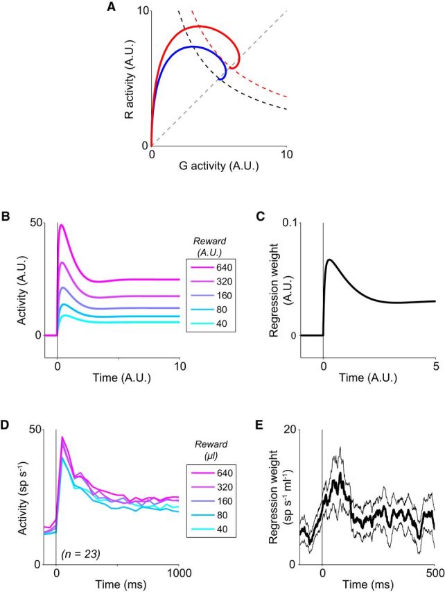
Single-option value dynamics. A, Value-dependent system trajectories in a single-option circuit. Example values inputs: V = 30 (blue), V = 40 (red). B, Dynamic value modulation in the normalization model, shown as R responses with varying value inputs. C, Time-varying strength of model value coding, calculated by regressing model responses on input value. D, Dynamic value coding in single-option LIP activity. Lines show population average LIP activity (n = 23 neurons) aligned to target onset, segregated by reward value. E, Time-varying strength of LIP value coding. Line shows population average value regression weight (±SEM). Consistent with model predictions, value coding across the population is stronger during the initial transient than at equilibrium.

In addition to value coding at equilibrium, the phase plane plots reveal higher peak excursions for larger value inputs. As evident in the activity trace, this pattern corresponds to value-dependent phasic transients at the onset of value input across a range of different values (Fig. 4B). Consistent with value coding during the transient, the peak activity in each condition R_max increases with input value. Notably, the extent of the initial activity excursion beyond the ultimate steady-state activity level is also value-dependent, resulting in a more pronounced phasic peak under larger value conditions. Mathematically, this occurs because the single-option R nullcline equation, as follows:

has the following properties:

The first inequality implies that the R nullcline shifts upward as value increases and underlies the general value-dependent increase in R neuron activity at all time points. The second inequality implies that the rate of value-mediated increase is smaller at higher levels of G activity; because inhibitory neuron activity is always greater at the equilibrium point than during the initial transient, it follows that the rate of change with respect to V of R* is less than that of R_max. This is evident as a stronger value modulation in peak activity compared with sustained activity in the model (Fig. 4C). The complete proof of this time-varying value coding is given in the Mathematical Analysis section below.

Multiple option dynamics: relative timing of direct and contextual information

A fundamental characteristic of the normalization computation is divisive scaling, typically by a quantity representing the summed activity of a large pool of neurons (Heeger, 1992; Carandini and Heeger, 2012). In decision-related brain areas, this normalization produces a relative value coding: the activity representing a given action increases with the value of that action and decreases with the value of alternative options (Rorie et al., 2010; Louie et al., 2011; Pastor-Bernier and Cisek, 2011). Thus, individual neurons carry value information about both targets within the neural RF that provide direct, feedforward activation and targets outside the RF that define the context of other possible choices. These findings suggest that individual neurons integrate value information about all available options, but little is known about how this is accomplished in cortical circuits.

Here, we show that the simple recurrent circuit model of normalization presented here predicts characteristic time courses for modulation by both direct and contextual value information. The intuition behind this time course difference is evident in the mechanism by which different kinds of value information reach a given R neuron in the model. The value of a specific option directly excites the associated R neuron via value-modulated input. In contrast, the value of other options influences that neuron only through a chain comprising input-driven R neuron activity and G neuron inhibition. Thus, the influence of the value of an alternative option should be suppressive and arise later in time. Empirically, delayed onset of contextual information is widely documented in sensory processing, and evident in reward-related processing during perceptual decision-making (Rorie et al., 2010).

To quantify these effects in the dynamic normalization model, we examined the behavior of a two-choice, four-neuron circuit (Fig. 5). As shown in Figure 5A, the activity representing a given option (R₁) is dependent on the values of both presented alternatives; consistent with a normalized value code, activity increases as a function of V₁ and decreases as a function of V₂. However, there are notable timing differences in the dynamics of direct versus contextual modulation, as quantified by multiple-regression analysis of the model output (Fig. 5B). Whereas the effect of option value (V₁) increases R₁ activity almost immediately, the suppressive influence of value context (V₂) begins only after a short delay. Furthermore, the time of peak value modulation occurs later for value context (t = 0.88 A.U.) compared with option value (t = 1.89 A.U.). This delay in model contextual processing emphasizes the role of inhibitory G neurons, which exhibit a delayed response to value input (Fig. 3C) and mediate the suppressive effect of alternative option value via lateral inhibition.

Figure 5.

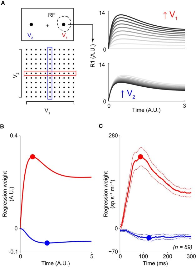
Multiple-option value dynamics. A, Contextual value manipulation. Left, Schematic of varying value inputs to a two-option, four-neuron version of the normalization model. Right, Example model responses. Consistent with value normalization, the activity of the R₁ unit increases as a function of V₁ and decreases as a function of V₂. Darker shading denotes higher corresponding value conditions. B, Differential timing in model value information processing. Sliding-window multiple-regression analysis of model activity over the full matrix of value conditions in A shows effect of direct (red) and contextual (blue) value on output R₁ activity. Notably, the peak extent of modulation occurs later for contextual value information. C, Differential timing in LIP value information processing. Mean regression coefficient (±SEM) of LIP neuron activity when either target value inside (red) or outside (blue) the response field is varied in multiple-option saccade tasks. Dots denote time of peak modulation, which occurs later for contextual value information.

Model validation: electrophysiological data

As discussed above, the dynamic normalization model makes specific qualitative predictions about the dynamic nature of value coding activity: (1) value coding during sustained delay-period activity, (2) value coding during the initial phasic transient, (3) time-varying strength of this value modulation, and (4) differential timing of direct and contextual value processing. To test the predictions of the dynamic normalization model, we examined the activity of LIP neurons in monkeys performing single- and multiple-target saccade tasks. Value modulation is commonly observed in LIP (Platt and Glimcher, 1999; Dorris and Glimcher, 2004; Sugrue et al., 2004; Louie and Glimcher, 2010; Rorie et al., 2010; Louie et al., 2011) but most studies of value-based decision-making have focused exclusively on delay-period modulation and little is known about the temporal dynamics of such coding.

We first examined LIP activity in a single-target value task, which avoids potentially confounding activity related to action selection (i.e., choice probability signals) in multiple alternative scenarios. In each trial, the monkey foveated a central fixation cue, viewed a peripheral target in the isolated neuron's RF, and completed a saccade to the target location. Successful saccades to the target produced a water reward whose magnitude was constant within a block of trials; reward magnitude was varied across blocks to determine the effect of value on the time course of LIP responses. In this single-alternative task, value modulates LIP firing rates throughout both the phasic and sustained phases of activity (Fig. 4D). As seen in the average population activity (n = 23 neurons), consistent value modulation occurs across both early and sustained periods of target presentation. Across the population, linear regression analysis (Fig. 4E) reveals that both phasic (t = 100–150 ms: mean β = 0.0095; p = 3.7 × 10⁻⁴, Wilcoxon signed rank test) and sustained (t = 950–1000 ms: mean β = 0.0035; p = 0.019) activity levels are dependent on value, with a significantly stronger modulation during the initial phasic transient than at steady-state (p = 0.0022, bootstrap test of difference of mean regression weights).

To test model predictions about the relative timing of direct and contextual value information, we next examined the dynamics of LIP value coding in multiple-option tasks (equilibrium activity previously analyzed and reported in by Louie et al., 2011; see Materials and Methods). In these tasks, the values of a target inside the RF and target(s) outside the RF were varied; we quantified via regression analyses how neural responses depended on direct RF value and contextual extra-RF value information. Consistent with the qualitative timing predictions of the model, the suppressive effect of contextual value is delayed relative to direct value activation. As evident in Figure 5C, the influence of RF value (red) rises immediately, significantly deviating from baseline (fixation) levels of modulation at 7 ms; in contrast, suppression by extra-RF value (blue) is unchanged for the first 25 ms and does not become significant until 44 ms (p < 0.05, bootstrap test of difference in mean regression coefficient). Furthermore, both the time of half-maximal modulation and the time of peak modulation occur significantly earlier for direct activation (t_half = 35 ms, t_peak = 87 ms) compared with contextual suppression (t_half = 60 ms, t_peak = 122 ms) processes (95% CI of difference between direct and contextual timing: Δt_half, [−49, −7]; Δt_peak, [−313, −2]). We note that similar reward effects have been shown in parietal neurons during a perceptual choice task (Rorie et al., 2010); our results confirm these previous findings and extend them to purely value-guided decision making.

Discounted divisive normalization

Although most normalization models scale the firing rate of a given neuron with respect to the instantaneous activity of a large normalization pool, others have been proposed that normalize over both the current and past activity of these neurons (Carandini and Heeger, 2012). In this approach, past activity is discounted with more recent activity weighted more heavily. Such models have been used to describe history-dependent processes including light adaptation in the retina and contrast adaptation in visual cortex but their implementation in decision-related circuits is unknown.

Our differential equations model incorporates an intrinsic dependence of current activity on past circuit activity because the firing rates are, by definition, time-dependent. Here, we show that the dynamic normalization model presented above implies that the firing rate at a fixed time is normalized by the firing rates at previous time steps in an exponentially weighted manner. In other words, our dynamical model naturally implements the extended time-dependent normalization model previously used to model adaptation (Wainwright et al., 2002; Carandini and Heeger, 2012; Sinz and Bethge, 2013). This discounted normalization equation is derived from Equations 1 and 2 by first discretizing the derivative (using Euler's Method), rescaling parameters, and relying on the linearity of the G′ equation, with the following result for a single (G,R) pair:

where the parameter α is between 0 and 1 and is related to the time step associated with discretization and the time constant τ. For multiple (G, R) pairs, this approach produces a double sum over both time and neuron pair.

This discounted formulation suggests that the firing rate at a given time depends on the firing rate at previous time steps in an exponentially decaying manner, with recent firing rates weighted most heavily. Critically, this circuit property suggests a neural mechanism for certain temporal forms of context-dependent choice behavior. Recent high-value choices, for example, would produce a persistent larger divisive scaling and persistently reduced firing rates in the current choice set, thus altering value-guided decisions. We note that because the current temporal structure of this model is qualitative in nature, it is unclear whether the time-scale in the current model is consistent with that necessary for context-dependent choice effects. These results are not dependent on the discretization, as we have also developed a continuous time version of the discounted form, with the summation replaced by a convolution with a decaying exponential function. The details of the derivations of both versions of our model are given in the following sections.

Mathematical analysis: equilibria in a single-option model

Here we provide the mathematical foundations for the results presented above. Instead of proving results for the specific normalization-based differential equations in the text, we consider more general families of differential equations of which the model equations are a special case; this theory indicates that the preceding results are not tied to a specific functional form of the differential equations. In what follows, the variable x corresponds to the variable G, and y corresponds to the variable R used in the main text. We have used these variables here to emphasize the generality of these results.

Theorem 1.

Consider the system of differential equations

defined for x ≥ 0, y ≥ 0 and satisfying the following conditions:

• α > 0 and β > 0,

• f is a continuously differentiable increasing function (f′(y) > 0) mapping an interval [a, ∞) onto [b, ∞) with a ≥ 0, b ≥ 0, and either a = 0 or b = 0.

• g is a continuously differentiable decreasing function (g′(x) < 0) mapping the interval [0, ∞) onto an interval (0, M], and

  

  Then the equations (10) have the following properties: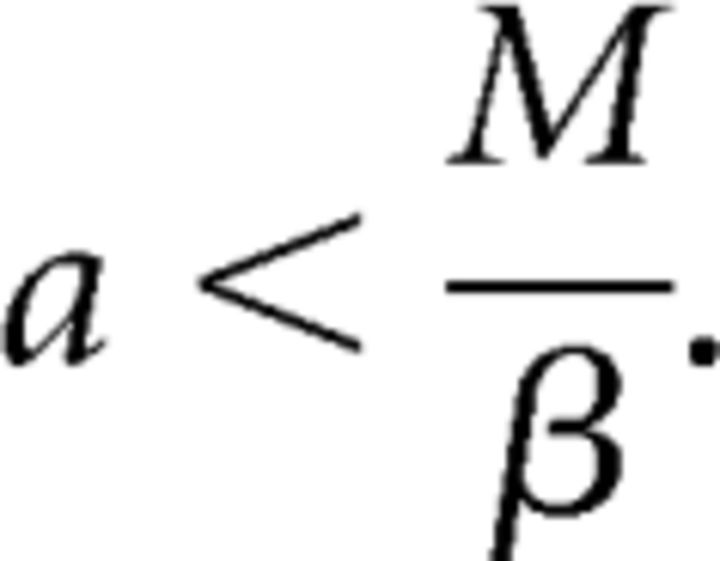

1. There exists a unique asymptotically stable equilibrium point (x*,y*) ∈ ℝ⁺ × ℝ⁺.

2. Any solution φ_t (x₀, y₀) with the initial condition: (x₀, y₀) ∈ R = $\left\{\left(x,y\right):0\le x\le \frac{f\left(M/\beta \right)}{\alpha }\text{and}0\le y\le \frac{M}{\beta }\right\}$ satisfies $\underset{t\to \infty }{{\displaystyle \lim }}$ φ_t(x₀, y₀) = (x*, y*).

3. If (x₀, y₀) ∈ [0,x*) × [0, y*), then there exists a t̄ > 0, such that y(t) has a local maximum at t̄.

Proof

We begin by showing that the system of equations (10) has a unique equilibrium point. The nullclines are given by x = f(y)/α and y = g(x)/β, and any equilibrium is the intersection of these two graphs.

Because f is invertible we can express the x-nullcline as y = f⁻¹(αx). Note that this latter function is monotonically increasing and f⁻¹:[b, ∞) → [a, ∞). Let

Because $\underset{x\to \infty }{{\displaystyle \lim }}$ g(x) = 0 and $\underset{x\to \infty }{{\displaystyle \lim }}$ f⁻¹(x) = ∞, there exists an x > b, such that H(x) = 0. First assume that b = 0, and hence f⁻¹(0) = a by assumption. Then,

By the intermediate value theorem, there exists x*, such that H(x*) = 0. Moreover, because H′(x) < 0, x* is the unique zero of H.

Now suppose that b ≠ 0 so that a = 0. Then,

and again we have a unique x*, such that H(x*) = 0. Clearly x* is the x-coordinate of an equilibrium point and thus we have shown system 10 has a unique equilibrium point.

The asymptotic stability of (x*, y*) is determined by evaluating the Jacobian matrix at (x*, y*) to get the following:

Because Tr J = −(α + β) < 0 and det J = αβ − f′(y*)g′(x*) > 0, it follows that both eigenvalues of J have a negative real part, and thus the equilibrium point is locally asymptotically stable.

We next prove Statement 2. It is easy to show that the compact rectangular region R is positively invariant. This implies that solutions with initial conditions in R exist for all t > 0, and thus these solutions have nontrivial ω-limit sets. Moreover, because:

for all x ≥ 0, y ≥ 0, it follows from Bendixon's criterion that there are no periodic orbits in this region. Thus all solutions interior to R limit on the equilibrium (x*, y*).

The proof of Statement 3 is also straightforward. If (x₀, y₀) ∈ [0,x*) × [0, y*), then the solution curve φ_t (x₀,y₀) exits this rectangle through the line y = y* and into the compact region bounded by this line, the y-axis, and the graph of y = g(x)/β with 0 ≤ x ≤ x*. Solution curves in this region must exit by crossing the y-nullcline at a value of y > y*. Thus y(t) has a local maximum at some value t = t₁ > 0.

Mathematical analysis: effect of changing value in a single-option model

We now turn our attention to families of differential equations satisfying the properties of Theorem 1. In particular, we consider the family of differential equations:

satisfying the conditions of Theorem 1 for all V > 0. In addition we assume that ∂g/∂V > 0, and a < M(V)/β for all V in some interval (V_min, V_max). Let A_V denote the open triangular shaped region bounded by the y-axis, and the x and y nullclines for a given value of V.

Theorem 2.

Consider the family of differential equations (11) that satisfy the conditions of Theorem 1, ∂g/∂V > 0, and a < M(V)/β for all V in some interval (V_min, V_max). Then,

1. The y-coordinate of the equilibrium point y*(V) is increasing, and

2. if V_min < V₁ < V₂ < V_max, then for all (x₀,y₀) ∈ A_v1

   

   where t̄_k is the minimal t > 0, such that π_y ○ φ(t̄_k,x₀,y₀;V_k) is a local maximum.

Proof

Statement 1 follows immediately from the fact that ∂g/∂V > 0, and f′(y) > 0.

Let V₁ < V₂, and let A = A_v1 ∩ A_v2. Let (x₀,y₀) ∈ A and define γ_k(t) = φ_t(x₀,y₀;V_k) for k = 1,2.

For all (x,y) ∈ A, the slope of each vector defined by (11) is given by the following:

Moreover, the following derivative:

describes the change in these slopes with respect to a change in the parameter V and if (x,y) ∈ A, then $\frac{\partial T}{\partial V}$ > 0. Thus the slopes of the vectors in this region increase with V.

Because T(x,y;V) > 0 and $\frac{\partial T}{\partial V}$ > 0 in A_, it follows that for V₁ and V₂ each vector in A is directed upward and to the right and T(x,y;V₂) > T(x,y;V₁). This implies that there exists ε > 0, such that for all t and s with 0 < t < ε and 0 < s < ε, then γ₂(t) > γ₁(t). In other words, the solution curve γ₂ lies above the solution curve γ₁ for sufficiently small t and s.

Now suppose, by way of contradiction, that the solution curves γ₁ and γ₂ intersect in A. Then there exists t̄ > 0 and s̄ > 0, such that:

in A. Because γ₂ initially lies above γ₁, it follows that:

But this contradicts the fact that $\frac{\partial T}{\partial V}$ > 0. Hence γ₂(t) lies above γ₁(s) when both solution curves lie in the region A.

This, combined with the fact y = g(x;V₁) is decreasing, implies that γ(t) intersects the nullcline y = g(x;V₁) at a greater value of y thanγ₁(s). Because γ₂(t) is still increasing and γ₁(s) is at its maximum, it follows that the maximum of γ₂ is greater than the maximum of γ₁.

Mathematical analysis: equilibria in multiple option models

We now turn our consideration to systems of differential equations based on those studied above. Let X ∈ ℝⁿ and Y ∈ ℝⁿ and consider the system of differential equations on ℝ²ⁿ as follows:

Let A = diag(α_i) and B = diag(β_i) be n × n positive, diagonal matrices. Let W = [ω_ij] be an n × n non-negative matrix and define the diagonal matrix W_d = [δ_ijω_ij], where:

Assume that F: ℝⁿ→ℝⁿ is continuously differentiable and has the form

with f_i(z) > 0 for all i. Similarly, G: ℝⁿ→ℝⁿ is continuously differentiable and has the following form:

with each g_i satisfying the conditions imposed on g in Theorem 1. Finally, recall that the norm of an n × n matrix M is given by the following:

Theorem 3.

If ‖W − W_d‖ is sufficiently small then system (12) has a unique asymptotically stable equilibrium in (ℝ⁺ × ℝ⁺)ⁿ.

Proof

When W = W_d then the equations (12) decouple to a system of n pairs of differential equations each satisfying the hypotheses of Theorem 1. Thus each pair of equations has a unique asymptotically stable equilibrium point (x_i^*,y_i^*) ∈ ℝ⁺ × ℝ⁺ for i = 1 to n. Thus, in this case, equations (12) also have a unique asymptotically stable equilibrium at (X̄,Ȳ), where X̄ = (x₁^*,…,x_n^*). and Ȳ = (y₁^*,…,y_n^*) Because (X̄,Ȳ) is structurally stable, it follows immediately that equations (12) also have a unique asymptotically stable equilibrium in some neighborhood of (X̄,Ȳ) for sufficiently small ‖W − W_d‖. See Guckenheimer and Holmes (1983) for a discussion of perturbations of structural stable systems of differential equations.

We note here that the above theorem is local in the sense that the persistence of the asymptotically stable equilibrium is only guaranteed for some “small” value of ε, where ‖W − W_d‖ < ε. Numerical simulations suggest that this value of ε is in fact fairly large. Simulations suggest that as long as ω_ij < 1 for all i and j, then the asymptotically stable equilibrium persists.

Mathematical analysis: derivation of the discounted normalization equations

Consider the system of differential equations as follows:

We begin by discretizing this system of equations via Euler's method with a step size of hτ with 0 < h < 1. This gives the discrete system:

where α = 1 − h and the parameters ω and V are rescaled from (13) by a factor of h.

Assume initial conditions of x₀ = 0 and y₀ > 0. It follows immediately that:

The next terms in the sequence are as follows:

By induction, we get the generalized x term of the following:

Substituting this into the y recurrence in (14) gives the following:

as desired.

Discussion

We show here that a simple dynamical model incorporating recurrent gain control and lateral connectivity captures fundamental aspects of early decision-related processing. Although this mathematical model is more abstract than biophysically realistic network models of decision circuits, it provides a number of qualitative predictions regarding value coding neural activity. This circuit exhibits both empirically observed normalized value coding at equilibrium and characteristic dynamics including sequential phasic-sustained activity, time-varying value modulation, and differential strength and timing of direct versus contextual information processing. Together, these findings suggest that multiple aspects of value coding can arise from intrinsic interactions of the local circuit and reinforce the importance of examining temporal aspects of the normalization process (Carandini and Heeger, 1994; Carandini et al., 1997; Mikaelian and Simoncelli, 2001; Reynaud et al., 2012).

Identifying the biological basis of value normalization is an essential step in understanding its role in neural coding and ultimately behavior. Normalization occurs in diverse brain areas and organisms, suggesting that the common element is the computation rather than a specific biophysical mechanism (Carandini and Heeger, 2012). For gain control in simpler systems, such as retinal photoreceptor light adaptation, normalization can be mediated by intracellular phenomena (Normann and Perlman, 1979). However, normalization processes involving a pooled signal summing over many neurons are likely mediated by a circuit-level mechanism. Feedforward mechanisms may drive normalization in certain circuits such as the housefly visual or fruit fly olfactory systems (Reichardt et al., 1983; Olsen et al., 2010), but the predominant candidate architecture for normalization in cortical areas is feedback connectivity. Recurrent connections are a characteristic feature of cortical circuits (Gilbert, 1983; Callaway, 1998; Douglas and Martin, 2004) and feedback inhibition plays a critical role in shaping cortical activity (Isaacson and Scanziani, 2011), possibly by balancing excitatory drive via divisive gain control (Chance and Abbott, 2000; Chance et al., 2002). Consistent with a feedback mechanism, we find that a simple network with recurrent and lateral inhibition replicates dynamic and equilibrium aspects of normalized value coding.

The strong similarity between theoretical predictions and empirical dynamics suggests that our basic model captures fundamental features of value normalization, but several important open questions remain. First, our model incorporates divisive scaling via recurrent inhibition but is agnostic about how this is implemented at the biophysical level. Shunting inhibition can implement divisive gain control (Carandini and Heeger, 1994; Carandini et al., 1997; Mitchell and Silver, 2003) but its role in empirical normalization remains debated (Holt and Koch, 1997) and other mechanisms, such as balanced excitation and inhibition, may be involved (Chance et al., 2002). Second, how value information reaches cortical areas like LIP is unknown. Such signals could arrive in a bottom-up manner from lower order sensory cortices or in a top-down manner from reward-coding frontal brain areas. Our model does not differentiate between these possibilities, and identifying the source of value information is a crucial target of further work. Finally, in addition to recurrent inhibition, cortical circuits exhibit additional complexities including laminar organization, recurrent excitation, and multiple interneuron subtypes. Although not necessary to generate the dynamic properties of early value coding, these features may be important in other aspects of decision processing; for example, recurrent excitation likely underlies the late winner-take-all dynamics that implement selection (Wang, 2002, 2008, 2012). A goal of our future research is to incorporate these features into richer models of the valuation process.

To date, empirical and theoretical studies have focused predominantly on neural activity in the latter stages of the decision process, when action-selective neurons begin to indicate choice outcome. Neural dynamics during this interval have been studied extensively in perceptual decision tasks and characterized with mathematical and network models based on the accumulation of noisy evidence over time. Such models typically are not applied to early decision-related neural activity: drift diffusion models characterize firing rates associated with a motion stimulus that appears after target onset (Roitman and Shadlen, 2002; Churchland et al., 2008) and network models often ignore early activity or assume that dynamics are inherited strictly from feedforward input (Wang, 2002; Furman and Wang, 2008). Our model suggests that divisive normalization operates early in the decision process, mediating value coding even during the initial sensory-associated transient. However, it is important to note that the normalization circuit described here does not implement winner-take-all selection; because the system reaches a value coding equilibrium, it does not exhibit the attractor state dynamics observed in networks with strong recurrent excitation. Thus, these results suggest that a full description of decision-making requires two dynamic processes: inhibition-mediated normalized value coding and excitation-mediated winner-take-all choice. Identifying the neural circuit components that implement these different computations in the same network will be a critical target of future research.

References

- Andersen RA, Buneo CA. Intentional maps in posterior parietal cortex. Annu Rev Neurosci. 2002;25:189–220. doi: 10.1146/annurev.neuro.25.112701.142922. [DOI] [PubMed] [Google Scholar]
- Bonin V, Mante V, Carandini M. The suppressive field of neurons in lateral geniculate nucleus. J Neurosci. 2005;25:10844–10856. doi: 10.1523/JNEUROSCI.3562-05.2005. [DOI] [PMC free article] [PubMed] [Google Scholar]
- Britten KH, Heuer HW. Spatial summation in the receptive fields of MT neurons. J Neurosci. 1999;19:5074–5084. doi: 10.1523/JNEUROSCI.19-12-05074.1999. [DOI] [PMC free article] [PubMed] [Google Scholar]
- Callaway EM. Local circuits in primary visual cortex of the macaque monkey. Annu Rev Neurosci. 1998;21:47–74. doi: 10.1146/annurev.neuro.21.1.47. [DOI] [PubMed] [Google Scholar]
- Carandini M, Heeger DJ. Summation and division by neurons in primate visual cortex. Science. 1994;264:1333–1336. doi: 10.1126/science.8191289. [DOI] [PubMed] [Google Scholar]
- Carandini M, Heeger DJ. Normalization as a canonical neural computation. Nat Rev Neurosci. 2012;13:51–62. doi: 10.1038/nrc3398. [DOI] [PMC free article] [PubMed] [Google Scholar]
- Carandini M, Heeger DJ, Movshon JA. Linearity and normalization in simple cells of the macaque primary visual cortex. J Neurosci. 1997;17:8621–8644. doi: 10.1523/JNEUROSCI.17-21-08621.1997. [DOI] [PMC free article] [PubMed] [Google Scholar]
- Chance FS, Abbott LF. Divisive inhibition in recurrent networks. Network. 2000;11:119–129. doi: 10.1088/0954-898X/11/2/301. [DOI] [PubMed] [Google Scholar]
- Chance FS, Abbott LF, Reyes AD. Gain modulation from background synaptic input. Neuron. 2002;35:773–782. doi: 10.1016/S0896-6273(02)00820-6. [DOI] [PubMed] [Google Scholar]
- Churchland AK, Kiani R, Shadlen MN. Decision-making with multiple alternatives. Nat Neurosci. 2008;11:693–702. doi: 10.1038/nn.2123. [DOI] [PMC free article] [PubMed] [Google Scholar]
- Dorris MC, Glimcher PW. Activity in posterior parietal cortex is correlated with the relative subjective desirability of action. Neuron. 2004;44:365–378. doi: 10.1016/j.neuron.2004.09.009. [DOI] [PubMed] [Google Scholar]
- Douglas RJ, Martin KA. Neuronal circuits of the neocortex. Annu Rev Neurosci. 2004;27:419–451. doi: 10.1146/annurev.neuro.27.070203.144152. [DOI] [PubMed] [Google Scholar]
- Furman M, Wang XJ. Similarity effect and optimal control of multiple-choice decision making. Neuron. 2008;60:1153–1168. doi: 10.1016/j.neuron.2008.12.003. [DOI] [PMC free article] [PubMed] [Google Scholar]
- Gilbert CD. Microcircuitry of the visual cortex. Annu Rev Neurosci. 1983;6:217–247. doi: 10.1146/annurev.ne.06.030183.001245. [DOI] [PubMed] [Google Scholar]
- Gnadt JW, Andersen RA. Memory related motor planning activity in posterior parietal cortex of macaque. Exp Brain Res. 1988;70:216–220. doi: 10.1007/BF00271862. [DOI] [PubMed] [Google Scholar]
- Guckenheimer J, Holmes P. Nonlinear oscillations, dynamical systems, and bifurcations of vector fields. New York: Springer; 1983. [Google Scholar]
- Heeger DJ. Normalization of cell responses in cat striate cortex. Vis Neurosci. 1992;9:181–197. doi: 10.1017/S0952523800009640. [DOI] [PubMed] [Google Scholar]
- Holt GR, Koch C. Shunting inhibition does not have a divisive effect on firing rates. Neural Comput. 1997;9:1001–1013. doi: 10.1162/neco.1997.9.5.1001. [DOI] [PubMed] [Google Scholar]
- Hunt LT, Kolling N, Soltani A, Woolrich MW, Rushworth MF, Behrens TE. Mechanisms underlying cortical activity during value-guided choice. Nat Neurosci. 2012;15:470–476. S1–3. doi: 10.1038/nn.3017. [DOI] [PMC free article] [PubMed] [Google Scholar]
- Isaacson JS, Scanziani M. How inhibition shapes cortical activity. Neuron. 2011;72:231–243. doi: 10.1016/j.neuron.2011.09.027. [DOI] [PMC free article] [PubMed] [Google Scholar]
- Jocham G, Hunt LT, Near J, Behrens TE. A mechanism for value-guided choice based on the excitation-inhibition balance in prefrontal cortex. Nat Neurosci. 2012;15:960–961. doi: 10.1038/nn.3140. [DOI] [PMC free article] [PubMed] [Google Scholar]
- Louie K, Glimcher PW. Separating value from choice: delay discounting activity in the lateral intraparietal area. J Neurosci. 2010;30:5498–5507. doi: 10.1523/JNEUROSCI.5742-09.2010. [DOI] [PMC free article] [PubMed] [Google Scholar]
- Louie K, Grattan LE, Glimcher PW. Reward value-based gain control: divisive normalization in parietal cortex. J Neurosci. 2011;31:10627–10639. doi: 10.1523/JNEUROSCI.1237-11.2011. [DOI] [PMC free article] [PubMed] [Google Scholar]
- Louie K, Khaw MW, Glimcher PW. Normalization is a general neural mechanism for context-dependent decision making. Proc Natl Acad Sci U S A. 2013;110:6139–6144. doi: 10.1073/pnas.1217854110. [DOI] [PMC free article] [PubMed] [Google Scholar]
- Mikaelian S, Simoncelli EP. Modeling temporal response characteristics of V1 neurons with a dynamic normalization model. Neurocomputing. 2001;38–40:1461–1467. [Google Scholar]
- Mitchell SJ, Silver RA. Shunting inhibition modulates neuronal gain during synaptic excitation. Neuron. 2003;38:433–445. doi: 10.1016/S0896-6273(03)00200-9. [DOI] [PubMed] [Google Scholar]
- Normann RA, Perlman I. The effects of background illumination on the photoresponses of red and green cones. J Physiol. 1979;286:491–507. doi: 10.1113/jphysiol.1979.sp012633. [DOI] [PMC free article] [PubMed] [Google Scholar]
- Ohshiro T, Angelaki DE, DeAngelis GC. A normalization model of multisensory integration. Nat Neurosci. 2011;14:775–782. doi: 10.1038/nn.2815. [DOI] [PMC free article] [PubMed] [Google Scholar]
- Olsen SR, Bhandawat V, Wilson RI. Divisive normalization in olfactory population codes. Neuron. 2010;66:287–299. doi: 10.1016/j.neuron.2010.04.009. [DOI] [PMC free article] [PubMed] [Google Scholar]
- Pastor-Bernier A, Cisek P. Neural correlates of biased competition in premotor cortex. J Neurosci. 2011;31:7083–7088. doi: 10.1523/JNEUROSCI.5681-10.2011. [DOI] [PMC free article] [PubMed] [Google Scholar]
- Platt ML, Glimcher PW. Neural correlates of decision variables in parietal cortex. Nature. 1999;400:233–238. doi: 10.1038/22268. [DOI] [PubMed] [Google Scholar]
- Rabinowitz NC, Willmore BD, Schnupp JW, King AJ. Contrast gain control in auditory cortex. Neuron. 2011;70:1178–1191. doi: 10.1016/j.neuron.2011.04.030. [DOI] [PMC free article] [PubMed] [Google Scholar]
- Reichardt W, Poggio T, Hausen K. Figure-ground discrimination by relative movement in the visual system of the fly: Part II. Towards the neural circuitry. Biol Cybern. 1983;46:1–30. doi: 10.1007/BF00595226. [DOI] [Google Scholar]
- Reynaud A, Masson GS, Chavane F. Dynamics of local input normalization result from balanced short- and long-range intracortical interactions in area V1. J Neurosci. 2012;32:12558–12569. doi: 10.1523/JNEUROSCI.1618-12.2012. [DOI] [PMC free article] [PubMed] [Google Scholar]
- Reynolds JH, Heeger DJ. The normalization model of attention. Neuron. 2009;61:168–185. doi: 10.1016/j.neuron.2009.01.002. [DOI] [PMC free article] [PubMed] [Google Scholar]
- Roitman JD, Shadlen MN. Response of neurons in the lateral intraparietal area during a combined visual discrimination reaction time task. J Neurosci. 2002;22:9475–9489. doi: 10.1523/JNEUROSCI.22-21-09475.2002. [DOI] [PMC free article] [PubMed] [Google Scholar]
- Rorie AE, Gao J, McClelland JL, Newsome WT. Integration of sensory and reward information during perceptual decision-making in lateral intraparietal cortex (LIP) of the macaque monkey. PLoS One. 2010;5:e9308. doi: 10.1371/journal.pone.0009308. [DOI] [PMC free article] [PubMed] [Google Scholar]
- Shadlen MN, Newsome WT. Neural basis of a perceptual decision in the parietal cortex (area LIP) of the rhesus monkey. J Neurophysiol. 2001;86:1916–1936. doi: 10.1152/jn.2001.86.4.1916. [DOI] [PubMed] [Google Scholar]
- Sinz F, Bethge M. Temporal adaptation enhances efficient contrast gain control on natural images. PLoS Comput Biol. 2013;9:e1002889. doi: 10.1371/journal.pcbi.1002889. [DOI] [PMC free article] [PubMed] [Google Scholar]
- Sugrue LP, Corrado GS, Newsome WT. Matching behavior and the representation of value in the parietal cortex. Science. 2004;304:1782–1787. doi: 10.1126/science.1094765. [DOI] [PubMed] [Google Scholar]
- Wainwright MJ, Schwartz O, Simoncelli EP. Natural image statistics and divisive normalization: modeling nonlinearity and adaptation in cortical neurons. In: Rao RPN, Olshausen BA, Lewicki MS, editors. Probabilistic models of the brain: perception and neural function. Cambridge, MA: MIT; 2002. pp. 203–222. [Google Scholar]
- Wang XJ. Probabilistic decision making by slow reverberation in cortical circuits. Neuron. 2002;36:955–968. doi: 10.1016/S0896-6273(02)01092-9. [DOI] [PubMed] [Google Scholar]
- Wang XJ. Decision making in recurrent neuronal circuits. Neuron. 2008;60:215–234. doi: 10.1016/j.neuron.2008.09.034. [DOI] [PMC free article] [PubMed] [Google Scholar]
- Wang XJ. Neural dynamics and circuit mechanisms of decision-making. Curr Opin Neurobiol. 2012;22:1039–1046. doi: 10.1016/j.conb.2012.08.006. [DOI] [PMC free article] [PubMed] [Google Scholar]
- Wilson HR, Humanski R. Spatial frequency adaptation and contrast gain control. Vision Res. 1993;33:1133–1149. doi: 10.1016/0042-6989(93)90248-U. [DOI] [PubMed] [Google Scholar]
- Zoccolan D, Cox DD, DiCarlo JJ. Multiple object response normalization in monkey inferotemporal cortex. J Neurosci. 2005;25:8150–8164. doi: 10.1523/JNEUROSCI.2058-05.2005. [DOI] [PMC free article] [PubMed] [Google Scholar]