A Flexible Sigmoid Function of Determinate Growth

Abstract

A new empirical equation for the sigmoid pattern of determinate growth, ‘the beta growth function’, is presented. It calculates weight (w) in dependence of time, using the following three parameters: t_m, the time at which the maximum growth rate is obtained; t_e, the time at the end of growth; and w_max, the maximal value for w, which is achieved at t_e. The beta growth function was compared with four classical (logistic, Richards, Gompertz and Weibull) growth equations, and two expolinear equations. All equations described successfully the sigmoid dynamics of seed filling, plant growth and crop biomass production. However, differences were found in estimating w_max. Features of the beta function are: (1) like the Richards equation it is flexible in describing various asymmetrical sigmoid patterns (its symmetrical form is a cubic polynomial); (2) like the logistic and the Gompertz equations its parameters are numerically stable in statistical estimation; (3) like the Weibull function it predicts zero mass at time zero, but its extension to deal with various initial conditions can be easily obtained; (4) relative to the truncated expolinear equation it provides more reasonable estimates of final quantity and duration of a growth process. In addition, the new function predicts a zero growth rate at both the start and end of a precisely defined growth period. Therefore, it is unique for dealing with determinate growth, and is more suitable than other functions for embedding in process‐based crop simulation models to describe the dynamics of organs as sinks to absorb assimilates. Because its parameters correspond to growth traits of interest to crop scientists, the beta growth function is suitable for characterization of environmental and genotypic influences on growth processes. However, it is not suitable for estimating maximum relative growth rate to characterize early growth that is expected to be close to exponential.

INTRODUCTION

Most annual agricultural crops are determinate, and their growth stops once they reach physiological maturity. For indeterminate crops, growth of their individual organs is not unlimited, even when environmental conditions remain favourable. The length of the growth period and the weight of ultimate growth, either for the determinate crop as a whole or for specific organs, are two important environment‐dependent traits. Crop physiologists and geneticists like to quantify the two traits to characterize genotypic variation in response to growth environments, thereby assisting breeders in the design of crop varieties for target environments. In plant simulation modelling, modellers often wish to quantify the dynamics of growth, enabling the daily growth rates being integrated to equal the expected ultimate weight at the end of the growing cycle (Read et al., 2002). A simple equation is needed to model and characterize the duration and the final weight of determinate growth processes.

Within the life cycle of an organ, a plant or a crop, the total growth duration can be divided into three sub‐phases: an early accelerating phase; a linear phase; and a saturation phase for ripening (Goudriaan and van Laar, 1994). Therefore, the growth pattern typically follows a sigmoid curve, and the growth rate a bell‐shaped curve. While the sigmoid pattern can be represented piecewise using an exponential, a linear and a convex equation sequentially (e.g. Lieth et al., 1996), a more elegant way is to use a curvilinear equation which gives a gradual transition from one phase to the next. For example, based on principles of light interception and leaf area expansion, Goudriaan and Monteith (1990) derived a single equation, the expolinear equation, for both the exponential and linear phases of crop growth:

where w is mass, t is time, t_o is the moment at which the linear phase effectively begins, and c_m and r_m are maximum growth rate in the ‘linear phase’ and maximum relative growth rate (RGR) in the ‘exponential phase’, respectively. To represent a deflection in growth towards the third phase, Goudriaan and Monteith (1990) suggested the truncated curve that terminates growth at the moment t_o + w_max/c_m, where w_max is the maximum value of w. This truncation creates an abrupt transition from the second to third phase, and predicts no growth at all during the third phase.

Goudriaan (1994) extended the expolinear equation for describing the pattern of leaf area index to allow a smooth second transition. The principle could also be applied to mass quantity. The expolinear equation with two smooth transitions is:

Equation (2) gives a symmetrical sigmoid pattern around time t_o + w_max/(2c_m). To distinguish it from the truncated equation, eqn (2) is referred to as the symmetrical expolinear function.

Alternative, but simpler, functions that can produce two smooth transitions in a single formula are the classical growth functions. The first is the well‐known logistic function (Verhulst, 1838):

where k is a constant that determines the curvature of the growth pattern, and t_m is the inflection point at which the growth rate reaches its maximum value. At time t_m, the RGR is k/2. As can be seen from eqn (3), the weight at t_m is half of its maximum value, w_max.

The logistic equation is symmetrical around time t_m. Richards (1959) introduced an additional parameter, v, to the logistic equation to deal with asymmetrical growth:

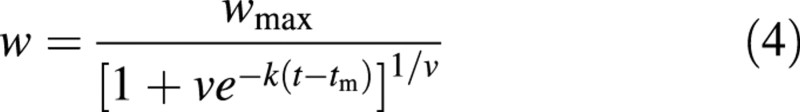
At time t_m, the absolute growth rate is maximal and the RGR is k/(1 + v). Equation (4) differs slightly from the original notation: by putting v in front of the exponential term the awkward ± conditional notation can be avoided (Goudriaan and van Laar, 1994). Clearly, eqn (4) becomes the logistic equation if v = 1.

The asymmetrical growth provided by the Richards equation [eqn (4)] is obtained at the cost of using one more parameter than is used in the logistic function. An alternative way to generate an asymmetrical growth curve is to use the Gompertz function (Gompertz, 1825; Winsor, 1932), which has only three parameters:

Equation (5) predicts that at the time of inflection, t_m, when the maximum growth rate is achieved, w is equal to w_max/e, and the RGR is equal to k. In fact, the Gompertz function is a special form of the Richards function when v → 0. This can be easily understood from the mathematical formula of approximation: 1 + x ≈ e^x if x → 0.

All of the above equations have the line w = 0 as their lower asymptote of sigmoid growth and, therefore, predict a positive non‐zero value for w at time t = 0. This is the case for a germinating plant or at the start of the growing season for a crop, but is not the case for some individual organs, e.g. seeds, which start with an initial weight of zero. A zero initial weight can be achieved by applying the Weibull function (Weibull, 1951):

where a and b are empirical constants, defining the shape of the response. Equation (6) differs slightly from the notation of the Weibull function for germination analysis (Dumur et al., 1990), which generally includes a parameter for a lag time.

In eqns (2)–(6), w_max is a parameter to be specified. However, none of these equations can explicitly predict an actual weight equal to w_max because they all have the line w = w_max as their upper asymptote when time tends to infinity. As a consequence, the length of the growth period is infinite in these equations, contravening the pattern of determinate growth. To achieve a set final weight at the end of a precisely defined growth period, a segmented terminate function is needed. While the truncated expolinear function can predict the final weight, it uses an abrupt transition and predicts a ‘sudden death’. To predict a smooth transition to the maximum weight, a non‐linear segment function that has a zero slope at the end of growth is required. Although cubic polynomials provide a zero slope at the end point, they are symmetrical, presenting a growth pattern with the maximum slope midway through the growing season. In addition, the coefficients of polynomial equations have no biological interpretation.

The aim of the present study is to present a new flexible asymmetrical sigmoid growth function, with clearly interpretable parameters, that can specify unambiguously the length of the growth period and smoothly predict w_max, the final weight of the determinate growth process.

MATERIALS AND METHODS

New growth function

The time course of the growth rate usually follows a unimodal bell‐shaped curve. To predict determinate growth, the growth rate has to be zero at the end point. This terminate growth pattern can be described by the beta distribution function, the probability density function that gives a family of flexible asymmetrical unimodal curves with two fixed end points (Johnson and Leone, 1964). The beta function was introduced by Yin et al. (1995) to describe the phasic development rate as a function of temperature. In analogy to the equation given by Yin et al. [1995; their equation (8b)], the full beta function for growth rate can be expressed as:

where c_m is the maximum growth rate, which is achieved at time t_m, and t_b and t_e are times at the beginning and end of the growth period, respectively. If the reference time is set as zero (t_b = 0), eqn (7) becomes simpler. By varying the parameter δ, various curvatures in the growth rate curve for the periods t < t_m and t > t_m can be produced (Yin et al., 1995).

Growth equations are usually presented in an integral form (Zeide, 1993) because instantaneous growth rates are not amenable to experimental collection. The equation for total weight in the present context can be obtained by integrating eqn (7) with respect to time t. However, a definite analytical solution to the integral of eqn (7) does not exist. Therefore, a simplification has to be made to arrive at a definite integral growth equation. To achieve such a general growth function which, like most existing growth functions, has only three parameters, we simply assume that parameter δ is equal to 1 [see eqn (A1) in Appendix]. Equation (A1) is equivalent to the beta equation for the temperature response of development rate, as simplified by Yan and Hunt (1999).

Based on eqn (A1), a new three‐parameter growth equation, with an initial weight of zero, can be formulated as (see Appendix):

where w_max is the maximum value of w, which is reached at time t_e.

Equation (8) obeys the constraints that w = 0 at the start of growth (i.e. t = 0), and w = w_max when growth is terminated (i.e. t = t_e). It can be applied to growth within the time span of 0 ≤ t ≤ t_e; otherwise, w has to be set as 0 if t < 0, and w_max if t > t_e. Because eqn (8) still produces an asymmetrical unimodal curve if t_e is exceeded (Fig. 1A), the equation with the extension that w is w_max if t > t_e is referred to as the beta sigmoid growth function. Unlike the truncated expolinear function, the beta growth function, whilst containing two segments, is smooth because the first derivatives of w with respect to t are zero at the joining point t = t_e.

Fig. 1. A, Time course of a growth process represented by the beta sigmoid growth function, as shown by the solid line from t = 0 until maximal weight (w_max) is achieved at the end of the growth period (t_e). Hereafter, the weight equals w_max. The dashed line is the mathematical extension of eqn (8) beyond t_e until time (2t_e – t_m), the second intercept of eqn (8) on the time axis. B, The corresponding time course of the absolute growth rate (solid line) and the relative growth rate (dashed line).

It is customary to give corresponding expressions for both absolute and relative growth rates associated with a growth equation. The beta growth rate function is presented as eqn (A1) where the maximum growth rate, c_m, is given by:

The equation for RGR is given by:

A typical time course of both absolute and relative growth rates is given in Fig. 1B. Because w is initially assumed to be zero (as in the Weibull equation), RGR is infinite at the start of growth; it then declines monotonically to zero at time t_e. Thereafter, both rates remain zero due to the restriction that w is w_max if t > t_e.

Comparison with some existing growth equations

The beta growth function is compared with the four widely used classical equations (logistic, Richards, Gompertz and Weibull) and the two expolinear equations in describing several growth processes. Parameters in all of the functions were derived from iterative non‐linear least‐square regression using the DUD method (Ralston and Jennrich, 1979), as implemented in the PROC NLIN of the SAS software package (SAS Institute Inc., 1988). The R²‐value of the linear regression between observed and predicted growth, and the mean absolute predictive discrepancy (MD), were used to indicate the goodness of fit. When equations are ‘nested’ (i.e. a simpler equation is the special case of a complex one), t‐ or F‐tests were used to evaluate whether the complex equation led to a significant improvement. This test was applied mainly to the Richards equation, which encompasses both the logistic and the Gompertz equation.

Data sets

Four data sets were used to evaluate the growth functions; these were chosen because they (1) represent growth processes at the organ, plant and crop level, respectively; and (2) show growth processes having various sigmoid shapes or show genotypic and environmental influences on growth traits.

The first data set refers to wheat (Triticum aestivum L.) grain growth in a glasshouse experiment involving plants of six genotypes (Table 1) grown in pots at two temperatures (Table 2) (W. Guo, pers. comm.). Grain weight was measured five to eight times during grain filling, by oven‐drying at 70 °C for at least 24 h.

Table 1.

Codes of the six wheat genotypes tested in a glasshouse experiment

Code	Genotype name
G1	CMH79A.955/4/AGA/3/4 × SN64/cno67/INIA66/5/NAC/6/CMH83.2517*
G2	VEE/CMH77A.917//VEE/6/CMH79A.955/4/AGA/3/4×SN64/CNO67//INIA66/5/*
G3	Baviacora
G4	ALTAR84/AE.SQ//OPATA*†
G5	ALTAR84/AE.SQ//OPATA*†
G6	SRMA/TUI*

* CIMMYT (International Maize and Wheat Improvement Centre) breeding lines;

^† These two genotypes are different selections of the same crosses.

Table 2.

Estimated parameter values (with s.e. in parentheses) of the beta growth function for grain filling in six wheat genotypes as tested in a glasshouse experiment at two temperatures (original data from W. Guo, pers. comm.)

Temperature (day/night)	Genotype*	wmax (mg grain–1)	tm (d)	te (d)	R 2	cm†(mg grain–1d–1)
T1: 20/15 °C	G1	48·09 (0·94)	19·54 (1·14)	41·37 (2·13)	0·980	1·72
	G2	52·20 (1·22)	19·92 (1·40)	42·95 (2·55)	0·973	1·79
	G3	50·53 (1·08)	13·05 (1·72)	37·27 (2·42)	0·975	1·96
	G4	48·09 (0·91)	12·53 (1·51)	35·50 (2·15)	0·979	1·95
	G5	50·98 (0·70)	13·23 (0·99)	31·96 (1·53)	0·987	2·36
	G6	42·51 (1·21)	14·58 (1·81)	34·59 (2·96)	0·956	1·79
T2: 25/20 °C	G1	39·73 (1·14)	14·47 (1·16)	28·01 (2·17)	0·962	2·15
	G2	44·96 (1·53)	14·87 (1·11)	25·94 (2·50)	0·949	2·74
	G3	42·54 (0·99)	9·79 (1·40)	24·80 (2·06)	0·978	2·48
	G4	41·98 (0·74)	10·34 (0·78)	21·60 (1·19)	0·986	2·88
	G5	45·17 (1·22)	9·75 (1·49)	27·11 (2·23)	0·979	2·40
	G6	39·90 (1·50)	10·31 (1·97)	25·77 (3·14)	0·954	2·24

* See Table 1 for genotype codes.

^† Maximum growth rate, calculated from eqn (9).

The remaining data sets have more data points, providing opportunities for more robust model testing. The second data set deals with accumulation of biomass of a single maize (Zea mays L.) plant. It is a classical data set for growth analysis (Hunt, 1981), taken from Kreusler et al. (1879). The data set gives a sigmoid pattern having a long expolinear phase before the end of growth.

The third data set was presented by Voisin et al. (2002) for a pea (Pisum sativum L.) crop. Data on aerial biomass were collected from field crops grown at four levels of nitrogen. Because pea biomass differed little among nitrogen levels, presumably due to the ability of pea plants to fix atmospheric nitrogen, the biomass values of the four treatments were averaged for evaluation. In this data set, the sigmoid growth was nearly symmetrical when time was expressed in degree‐days (°Cd).

The fourth data set comes from the growth of a field winter wheat crop (Gregory et al., 1978). Because fewer measurements were made on root systems, only data of aerial biomass were used. The time variable was given as days after sowing. The long growth lag due to low temperatures during winter and early spring produced a strongly skewed sigmoid growth pattern.

RESULTS

Parameter values of the beta growth function fitted to the growth data of wheat kernels are given in Table 2. The equivalent visual illustration of the fitting is shown in Fig. 2. The function accurately described the dynamics of change in dry weight of growing grains, with R²‐values > 0·94. Estimated values of w_max, t_m, t_e and c_m differed among the six genotypes tested and between the two temperature conditions (Table 2). However, the equation underestimated the first observation in most cases (Fig. 2).

Fig. 2. Observed (mean of three sampled culms at each time) time courses (points) and those described by the beta growth function (curve) of grain dry weight for six wheat genotypes (Table 1) grown in glasshouse at two temperatures (Table 2). Estimated parameter values are shown in Table 2. Observed data are from W. Guo (pers. comm.).

Because of the 12 genotype × temperature combinations, it is not feasible to show curve‐fitting results in tables and figures for the other six equations individually. To compare these equations, an overall evaluation of pooled results of estimated against observed grain weights is given in Table 3. All growth functions were capable of describing the dynamics in dry weight of growing grains (R² > 0·96 and MD < 2·1 mg). Similar to the beta function, the Gompertz and the Weibull equations also underestimated the first grain mass measurement (results not shown).

Table 3.

Overall evaluation of the seven growth functions in describing wheat grain‐filling data, by linear regression of predicted (y) vs. observed (x) grain weights and its R²‐value, and by the mean absolute predictive discrepancy (MD)

Model	Regression	R 2	MD (mg)
Truncated expolinear	y = 1·062 + 0·969x	0·971	1·984
Symmetrical expolinear	y = 0·669 + 0·978x	0·975	1·899
Logistic	y = 0·860 + 0·974x	0·973	1·931
Richards	y = 0·968 + 0·972x	0·974	1·906
Gompertz	y = 0·296 + 0·988x	0·970	2·100
Weibull	y = –0·053 + 0·997x	0·972	2·062
Beta	y = 0·294 + 0·988x	0·973	1·987

The seven equations have one common parameter, w_max. Compared with the estimate by the beta function, the truncated expolinear function gave a slightly lower estimate of w_max, while the other five equations using w = w_max as the asymptote gave a higher estimate of w_max (results not shown). The higher estimate of w_max by the Gompertz equation was especially conspicuous (Fig. 3A). Of the seven equations, only the beta and the truncated expolinear functions give an estimate for the real length of the grain‐filling period. Because the estimate by the truncated expolinear function is, in fact, the length of the early exponential and subsequent linear phase, the length estimated by this function is shorter than that given by the beta function (Fig. 3B).

Fig. 3. Comparison of maximum grain weight estimated by beta and Gompertz functions (A), and of grain filling duration estimated by beta and truncated expolinear functions (B). Observed experimental data are from W. Guo (pers. comm.). Diagonal broken lines show the 1 : 1 relationship.

Parameter values of the seven growth functions fitted to the data of Kreusler et al. (1879), Voisin et al. (2002) and Gregory et al. (1978) are given in Table 4. The visual illustration of the fitting by the beta function is shown in Fig. 4. Equivalent graphs for other functions are omitted because all functions achieved reasonable fits and therefore resulted in similar sigmoid curves.

Table 4.

Estimated parameter values (with s.e. in parentheses) of the seven growth functions fitted to the data for total biomass of a maize plant (Kreusler et al., 1879), for above‐ground biomass of a pea crop (Voisin et al., 2002), and for above‐ground biomass of a winter wheat crop (Gregory et al., 1978)

		Maize plant		Pea crop		Winter wheat crop
Model	Parameter	Estimate	Unit	Estimate	Unit	Estimate	Unit
Truncated expolinear	w max	123·36 (1·54)	g per plant	1196·00 (16·99)	g m–2	1247·96 (37·62)	g m–2
	t o	58·62 (1·71)	d	478·68 (40·77)	°Cd	181·47 (7·62)	d
	c m	2·69 (0·15)	g per plant d–1	1·57 (0·11)	g m–2 (°Cd)–1	17·45 (2·35)	g m–2 d–1
	r m	0·158 (0·021)	d–1	0·008 (0·002)	(°Cd)–1	0·077 (0·033)	d–1
	R 2	0·9983		0·9939		0·9852
	MD	1·2796	g per plant	26·395	g m–2	40·987	g m–2
Symmetrical expolinear	w max	126·95 (4·01)	g per plant	1248·47 (27·51)	g m–2	1252·41 (44·19)	g m–2
	t o	57·15 (2·02)	d	480·24 (65·83)	°Cd	199·69 (62·73)	d
	c m	2·61 (0·21)	g per plant d–1	1·63 (0·2741)	g m–2 (°Cd)–1	39·35 (196·93)	g m–2 d–1
	r m	0·249 (0·118)	d–1	0·009 (0·003)	(°Cd)–1	0·071 (0·044)	d–1
	R 2	0·9968		0·9940		0·9874
	MD	2·0471	g per plant	27·276	g m–2	44·160	g m–2
Logistic	w max	134·51 (4·81)	g per plant	1279·08 (27·53)	g m–2	1289·08 (43·17)	g m–2
	t m	83·27 (1·23)	d	877·64 (13·85)	°Cd	216·30 (1·95)	d
	k	0·090 (0·007)	d–1	0·005 (0·0003)	(°Cd)–1	0·061 (0·006)	d–1
	R 2	0·9954		0·9934		0·9875
	MD	2·2299	g per plant	30·207	g m–2	41·097	g m–2
Richards	w max	141·87 (11·74)	g per plant	1268·55 (39·55)	g m–2	1255·83 (46·56)	g m–2
	t m	81·55 (2·13)	d	877·32 (29·08)	°Cd	220·01 (4·38)	d
	k	0·069 (0·021)	d–1	0·006 (0·001)	(°Cd)–1	0·081 (0·027)	d–1
	v	0·502 (0·450)	–	1·157 (0·449)	–	1·776 (0·975)	–
	R 2	0·9956		0·9935		0·9880
	MD	1·9312	g per plant	30·316	g m–2	36·526	g m–2
Gompertz	w max	156·65 (10·42)	g per plant	1417·43 (57·79)	g m–2	1395·33 (82·25)	g m–2
	t m	79·22 (1·82)	d	786·42 (20·01)	°Cd	207·95 (2·52)	d
	k	0·047 (0·005)	d–1	0·003 (0·0002)	(°Cd)–1	0·036 (0·005)	d–1
	R 2	0·9952		0·9910		0·9833
	MD	2·1919	g per plant	33·674	g m–2	50·861	g m–2
Weibull	w max	128·12 (3·84)	g per plant	1258·62 (28·90)	g m–2	1237·88 (34·17)	g m–2
	a	2·51×10–11*	d–3·450	3·326×10–10†	(°Cd)–3·172	8·848×10–23*	d–9·381
	b	3·450 (0·318)	–	3·172 (0·150)	–	9·381 (0·836)	–
	R 2	0·9961		0·9938		0·9871
	MD	1·8942	g per plant	28·576	g m–2	39·643	g m–2
Beta	w max	123·49 (2·38)	g per plant	1213·30 (17·57)	g m–2	1235·48 (34·76)	g m–2
	t m	89·0 (0·76)	d	936·43 (10·70)	°Cd	229·60 (1·97)	d
	t e	108·47 (1·63)	d	1384·77 (26·89)	°Cd	257·03 (3·80)	d
	R 2	0·9968		0·9949		0·9851
	MD	1·6624	g per plant	25·334	g m–2	40·739	g m–2

MD, mean absolute predictive discrepancies.

* Standard error not given in the SAS output because the value was too low.

Fig. 4. Observed time courses (points) and those described by the beta growth function (curve) of the biomass for the whole maize plant (A, data from Kreusler et al., 1879), for pea crops (B, data from Voisin et al., 2002), and for winter wheat crops (C, data from Gregory et al., 1978). Estimated parameter values are shown in Table 4.

For the classical data set of Kreusler et al. (1879) on maize plant growth, growth functions represented the observed trend well (R² > 0·995, MD < 2·23 g; Table 4). Compared with others, the truncated expolinear function fitted slightly better to this data set, which included a long expolinear phase before the end of growth. As found for the grain‐filling process in wheat, equations using w = w_max as the asymptote gave a higher estimate of w_max than the beta or the truncated expolinear function, particularly the Gompertz equation (Table 4). The truncated expolinear function predicted the growth period as 104·5 d, slightly lower than that predicted by the beta function (108·5 d).

All seven functions fitted well to the data sets of Voisin et al. (2002) and Gregory et al. (1978) (Table 4). Again, the Gompertz equation predicted an appreciably higher w_max than other equations for both crops. The truncated expolinear function predicted the growth duration as 1242·4 °Cd for the pea crop and 253·0 d for the winter wheat crop, again somewhat shorter than values predicted by the beta growth function.

The present analysis involved a total of 15 curve fittings to each function. For the 15 fittings to the Richards equation, in no case did the value of its parameter v differ significantly from 1 (P > 0·05), and in only two cases (the pea data set and G5T1 for grain filling in wheat) did the value of v differ from zero (P < 0·05). Therefore, in nearly all cases, the Richards equation resulted in no significant improvement over the logistic equation, or over the Gompertz equation.

DISCUSSION

The beta growth function as a new class of growth equation

Zeide (1993) reviewed 12 promising equations, including popular ones such as the logistic, the Gompertz, the Richards and the Weibull equations. Given the fact that growth results from two opposing factors, namely the intrinsic tendency towards unlimited increase, and restraints imposed by environmental resistance and ageing, Zeide transformed the existing equations so that components corresponding to these two factors were exposed. His analysis (by differentiation, decomposition into the division components and taking logarithms) revealed that most existing growth equations did indeed consist of two modules, expansion and decline, encapsulating the positive and negative factors of growth, respectively. The expansion module is driven by plant size, and the decline module by age. The form of the expansion module is common to many equations. The decline module can be either an exponential or a power function. Accordingly, there are two basic forms behind growth equations: exponential decline form and power decline form. As evident from eqn (A1), both modules are driven by age in our function. The expansion module is a power function whereas the decline module is a linear function of the same variable. In this respect, the equation presented here is not only a new equation but a new class of growth equations. However, it is difficult to provide either direct or indirect evidence justifying the linear form of the decline module. This is because growth decline cannot be measured directly, or from analysis, e.g. plotting the ratio of the weight increase (dw/dt) to the expansion module of eqn (A1) against age, since values of parameters t_m and t_e cannot be assessed accurately from data prior to curve fitting.

Extension of the beta growth function to deal with various initial conditions

One property of the beta growth function, eqn (8), is that, like the Weibull equation, it always predicts the initial weight as zero. Other growth functions assume a certain initial value at the beginning of growth; this is reasonable for crops or plants because a crop or a plant does have a small initial weight at emergence as a consequence of sown seeds. The absence of a certain initial value in eqn (8) also explains why, in many cases (Fig. 2), the beta growth function underestimated grain weight at the first measurement, owing to an estimated delay of a few days in observing the actual start of flowering (W. Guo, pers. comm.). Nevertheless, for situations where the initial phase is important, the beta growth function can easily be extended:

where w_b is initial weight, and t_b is the moment at which growth begins. Equation (11) is the integral of eqn (7) with δ = 1, using the condition that w = w_b if t = t_b. The equation predicts a sigmoid growth pattern within the time span of t_b ≤ t ≤ t_e and allows for any reference time and initial weight. Unlike eqn (8), eqn (11) does not give an infinite RGR at the start of growth, i.e. at time t_b, so long as w_b is not zero. However, an over‐fitting might occur if both w_b and t_b are considered as parameters. For instance, the fitting of our data to eqn (11), supplemented with the condition that w = w_b if t < t_b, and w = w_max if t > t_e, did not yield simultaneous estimates of w_b and t_b differing significantly from zero (P > 0·05) because of high standard errors of their estimates. Only when either w_b or t_b was fixed at a certain (e.g. the observed) value, did the fitting yield a significant non‐zero t_b or w_b in some cases. In most cases the more simple formula, eqn (8), is sufficient if the emphasis is not on the very first stage.

Flexibility of the beta growth function

The logistic function is symmetrical around t_m. The Richards function is flexible and has often been used to describe various asymmetrical growth patterns (e.g. Zhu et al., 1988), but at the cost of using an additional parameter as compared with the logistic function. Both the Gompertz and the Weibull functions have the same number of parameters as the logistic function, and predict asymmetrical growth. However, they are not sufficiently flexible. For example, a symmetrical curve cannot be generated from these two functions by varying their parameter values. The Gompertz function is the special form of the Richards function when v → 0, and describes an asymmetrical sigmoid pattern with the point of inflection close to w_max/e. The fact that the Gompertz function consistently had the lowest R²‐values and the highest MD values (Tables 3 and 4), and tended to overestimate w_max (Fig. 3A; Table 4), may be due to this intrinsic inflexibility.

The beta growth function, eqn (8), can produce a family of asymmetrical growth curves within the span 0 ≤ t < t_e by varying the value of t_m (Fig. 5). An extreme example is when the maximum growth rate is achieved at the beginning of growth (t_m = 0). Equation (8) then becomes a quadratic equation without the constant term:

Fig. 5. Illustration of the flexibility of the beta growth function, eqn (8), in representing various sigmoid curves by varying the value of t_m within the range: 0 ≤ t_m < t_e. Curves from the quadratic to a nearly single pulse at t_e correspond to predictions by setting t_m = 0, 0·375t_e, 0·5t_e, 0·625t_e, 0·75t_e, 0·875t_e, 0·95t_e and 0·99975t_e, respectively.

In such a case (i.e. t_m = t_b), the more general beta function, eqn (11), then becomes:

The other extreme case is when the maximum growth rate is achieved towards the end of the growth period (t_m → t_e). The beta growth function then predicts an extremely skewed growth pattern towards a single pulse at t_e (Fig. 5). The symmetrical form of the beta growth function can be obtained by setting t_m as t_e/2, and eqn (8) becomes a cubic polynomial without the constant and linear terms:

The symmetrical form of eqn (11), with t_m = t_b + (t_e – t_b)/2, is a general cubic polynomial:

Therefore, the beta function represents a generalized polynomial equation, just as the Richards equation represents a generalized logistic equation. Cubic polynomial equations are not considered as general growth functions because their coefficients are lacking any biological interpretation (Zeide, 1993). But when polynomial equations are expressed as eqns (13A) and (13B), the meaning of parameters does show up. Equation (13) is the simplest expression that has a zero slope at the beginning and end of growth. Jones et al. (1979) found that cubic polynomial equations were better than the logistic and Gompertz equations in describing the process of grain filling in rice (Oryza sativa L.). Despite having only two parameters, eqn (13A), supplemented with the condition that w = w_max if t > t_e, also fitted well to the data of wheat grain growth as used in our study (results not shown). In their model for examining the impact of grazing on heaths, Read et al. (2002) used the differential form of eqn (13B) to represent heather shoot production in the case of no grazing.

Stability of model parameters

In terms of parameter number, the seven growth functions evaluated in the present study can be divided into two groups, three‐ vs. four‐parameter equations. In many cases, some estimated parameters were found to be statistically insignificant in the four‐parameter equations. For example, in the case of the wheat grain‐filling data set, the estimated parameter r_m in the two expolinear functions did not differ from zero (P > 0·05). The estimated value of r_m or c_m in eqn (2), when fitted to the data of Gregory et al. (1978), had high standard errors (Table 4) and was therefore insignificant (P > 0·05). The biological meaning of r_m and c_m requires that their value is not zero.

Despite its flexibility, the Richards equation has often been criticized: the shape parameter, v, has no obvious biological interpretation and is so unstable numerically that its estimate becomes useless (Zeide, 1993). For the data sets used in the present analysis involving a total of 15 curve fittings, in no case did the Richards equation achieve a statistically significant improvement over the logistic equation (P > 0·05), and in only two cases did it improve on the Gompertz equation (P < 0·05).

Like the logistic and the Gompertz equation, the beta growth function has three parameters, all of which are biologically interpretable and statistically significant in the present analysis (P < 0·01). The values of parameters in the beta function may be roughly judged from visual inspection of data. Parameters having a straightforward meaning are advantageous for statistical parameterization of non‐linear equations, if the parameters cannot be estimated through least‐squares regression of linearized forms. Parameters of such non‐linear functions have to be estimated by using an iterative regression approach, such as PROC NLIN (SAS Institute Inc., 1988), which requires an initial estimate of the parameters. We encountered problems in providing initial values for parameters a and b in the Weibull function because their meanings are confounded: the unit of parameter a depends on the value of parameter b, such as day^–b or (°Cd)^–b. The initial parameter values of this equation can only be provided by trial and error.

Use of the beta growth function

Many equations have been proposed to describe sigmoid growth (Zeide, 1993), and new equations are still being developed (e.g. Birch, 1999). To our knowledge, there is no existing sigmoid equation suitable for exact estimation of final biomass and duration of determinate growth. Our function is well suited in this respect, and is better than the truncated expolinear function because it can smoothly predict w_max as the final weight at the end of growth. While simplifications were made in its derivation, the beta growth function accurately described various growth dynamics (Figs 2 and 4). Because it has only three parameters, all with a straightforward biological meaning, the function is suitable for characterizing genotypic differences in, or environmental influences on, growth processes. This is clearly shown in the example of wheat grain growth (Table 2; Fig. 2), where genetic differences among the six genotypes regarding growth traits (grain filling duration, grain weight, maximum or mean grain filling rate) are immediately apparent, as is the effect of temperature on these traits. Needless to say, to obtain a reliable estimate of these traits, the observed data should cover the whole sigmoid range, preferably with some data points after the end of growth.

The beta growth function’s differential form, i.e. eqn (A1) with c_m calculated by eqn (9), can be used to quantify the dynamics of the strength of growing sinks (e.g. seeds) in process‐based crop simulation models. Classical (such as logistic) equations have often been used to describe the dynamics of the strength of seeds as sinks to absorb assimilates in such simulation models (e.g. Bindraban, 1997). The beta growth function is more suitable for this purpose, because (1) it predicts zero growth rate at both the onset and end of growth; and (2) it can specify seed weight and its growth duration, allowing a full weight to be reached precisely within the phenology quantified in a crop model.

The beta growth function predicts an accelerating, but not mathematically exponential, early growth. Classical growth analysis assumed that at small sizes, growth processes are exponential or growth rate is proportional to mass (Hunt, 1981). The intrinsic rate of increase of the early exponential growth, RGR, is treated as an important characteristic of particular conditions or genotypes. In such an analysis, the suitability of a growth function for estimating maximum RGR is an important part of its function (Birch, 1999). Like the Weibull function, the beta growth function, eqn (8), has a zero value at time zero, giving an infinite value of RGR at the start of growth (Fig. 1B). The full form of the beta growth function, eqn (11), does not ensure that the maximum RGR occurs at t_b. Therefore, the beta function, like the Weibull or the Gompertz equation, is not suitable for characterizing seedling growth in plant growth analysis. In this respect, expolinear growth equations have the advantage that the maximum RGR is one of their parameters. Furthermore, the beta growth function has no theoretical process basis. Again, expolinear equations have an advantage, especially when applied to a crop or vegetation as an alternative to a more complex process‐based simulation model (Goudriaan, 1994), because they are derived from the quantitative knowledge of sub‐processes such as light interception and leaf area expansion. Nevertheless, the beta growth function’s flexibility in representing various sigmoid patterns, its ease and stability in statistical parameterization, and its ability to estimate unambiguously the final biomass and the length of the growth period warrant its use as a new tool for quantitative analysis of growth processes.

ACKNOWLEDGEMENTS

This work was supported by the STW part of the Netherlands Organisation for Scientific Research through the PROFETAS (PROtein Foods, Environment, Technology, And Society) programme. We gratefully acknowledge Dr W. Guo for providing the data set of his wheat glasshouse experiment, and Drs C. P. D. Birch and B. Zeide for critical reviewing of the manuscript.

APPENDIX

Mathematical derivation of eqn (8)

If the reference time is set as t_b = 0 and parameter δ is set to 1, the beta function, eqn (7), for describing the time course of growth rate, becomes:

where c_m is the maximum growth rate, which is achieved at time t_m. The growth equation based on eqn (A1) is:

The solution to this integral can be readily derived or found in most tables of standard integrals in a mathematical handbook:

Equation (A3) does not add an integral constant at the end, because this constant is determined as zero from the condition that w = 0 if t = 0.

Most growth functions describe w in terms of w_max. The value of w_max can be calculated from the definite integral of eqn (A1) for the period between 0 and t_e, or from eqn (A3) by setting t = t_e:

Division of eqn (A3) by eqn (A4) gives:

An appropriate re‐formulation of eqn (A5) results in eqn (8).

Received: 21 June 2002; Returned for revision: 30 August 2002; Accepted: 6 November 2002    Published electronically: 19 December 2002

References

- BindrabanPS.1997. Bridging the gap between plant physiology and breeding: identifying traits to increase wheat yield potential using systems approaches. PhD Thesis, Wageningen Agricultural University, The Netherlands. [Google Scholar]
- BirchCPD.1999. A new generalized logistic sigmoid growth equation compared with the Richards growth equation. Annals of Botany 83: 713–723. [Google Scholar]
- DumurD, Pilbeam CJ, Craigon J.1990. Use of the Weibull function to calculate cardinal temperatures in faba bean. Journal of Experi mental Botany 41: 1423–1430. [Google Scholar]
- GompertzB.1825. On the nature of the function expressive of the law of human mortality, and on a new mode of determining the value of life contingencies. Philosophical Transactions of the Royal Society 182: 513–585. [DOI] [PMC free article] [PubMed] [Google Scholar]
- GoudriaanJ.1994. Using the expolinear growth equation to analyse resource capture. In: Monteith JL, Scott RK, Unsworth MH, eds. Resource capture by crops Nottingham: Nottingham University Press, 99–110. [Google Scholar]
- GoudriaanJ, Monteith JL.1990. A mathematical function for crop growth based on light interception and leaf area expansion. Annals of Botany 66: 695–701. [Google Scholar]
- GoudriaanJ, van Laar HH.1994. Modelling potential crop growth processes. Dordrecht: Kluwer Academic Publishers. [Google Scholar]
- GregoryPJ, McGown M, Biscoe PV, Hunte B.1978. Water relations of winter wheat. 1. Growth of the root system. Journal of Agricultural Science 91: 91–102. [Google Scholar]
- HuntR.1981. Studies in biology no. 96: plant growth analysis. London: Edward Arnold (Publishers) Limited. [Google Scholar]
- JohnsonNL, Leone FC.1964. Statistics and experimental design in engineering and the physical sciences. Vol. 1. New York: John Wiley & Sons, Inc. [Google Scholar]
- JonesDB, Peterson ML, Geng S.1979. Association between grain filling rate and duration and yield components in rice. Crop Science 19: 641–644. [Google Scholar]
- KreuslerU, Prehn A, Hornberger R.1879. Beobachtungen über das Wachstum der Maispflanze (Bericht über die Versuche vom Jahre 1878). Landwirtschaftliche Jahrbücher 8: 617–622. [Google Scholar]
- LiethJH, Fisher PR, Heins RD.1996. A phasic model for the analysis of sigmoid patterns of growth. Acta Horticulturae 417: 113–118. [Google Scholar]
- RalstonML, Jennrich RI.1979. DUD, a derivative‐free algorithm for nonlinear least squares. Technometrics 1: 7–14. [Google Scholar]
- ReadJM, Birch CPD, Milne JA.2002. HeathMod: a model of the impact of seasonal grazing by sheep on upland heaths dominated by Calluna vulgaris (heather). Biological Conservation 105: 279–292. [Google Scholar]
- RichardsFJ.1959. A flexible growth function for empirical use. Journal of Experimental Botany 10: 290–300. [Google Scholar]
- SAS Institute Inc.1988. SAS user’s guide: statistics, version 6·04 edition. Cary, North Carolina: SAS Institute Inc. [Google Scholar]
- VerhulstPF.1838. A note on population growth. Correspondence Mathematiques et Physiques 10: 113–121 (in French). [Google Scholar]
- VoisinA‐S, Salon C, Munier‐Jolain NG, Ney B.2002. Effect of mineral nitrogen on nitrogen nutrition and biomass partitioning between the shoot and roots of pea (Pisum sativum L.). Plant and Soil 242: 251–262. [Google Scholar]
- WeibullW.1951. A statistical distribution function of wide applicability. Journal of Applied Mechanics 18: 293–297. [Google Scholar]
- WinsorCP.1932. The Gompertz curve as a growth curve. Proceedings of the National Academy of Sciences of the United States of America 18: 1–8. [DOI] [PMC free article] [PubMed] [Google Scholar]
- YanW, Hunt LA.1999. An equation for modelling the temperature response of plants using only the cardinal temperatures. Annals of Botany 84: 607–614. [Google Scholar]
- YinX, Kropff MJ, McLaren G, Visperas RM.1995. A nonlinear model for crop development as a function of temperature. Agricultural and Forest Meteorology 77: 1–16. [Google Scholar]
- ZeideB.1993. Analysis of growth equations. Forest Science 39: 594–616. [Google Scholar]
- ZhuQ, Cao X, Luo Y.1988. Growth analysis on the process of grain filling in rice. Acta Agronomica Sinica 14: 182–193 (in Chinese with English abstract). [Google Scholar]
Associated Data
This section collects any data citations, data availability statements, or supplementary materials included in this article.