Using Structural Equation Modeling to Assess Functional Connectivity in the Brain: Power and Sample Size Considerations

Abstract

The present study assessed the impact of sample size on the power and fit of structural equation modeling applied to functional brain connectivity hypotheses. The data consisted of time-constrained minimum norm estimates of regional brain activity during performance of a reading task obtained with magnetoencephalography. Power analysis was first conducted for an autoregressive model with 5 latent variables (brain regions), each defined by 3 indicators (successive activity time bins). A series of simulations were then run by generating data from an existing pool of 51 typical readers (aged 7.5-12.5 years). Sample sizes ranged between 20 and 1,000 participants and for each sample size 1,000 replications were run. Results were evaluated using chi-square Type I errors, model convergence, mean RMSEA (root mean square error of approximation) values, confidence intervals of the RMSEA, structural path stability, and D-Fit index values. Results suggested that 70 to 80 participants were adequate to model relationships reflecting close to not so close fit as per MacCallum et al.'s recommendations. Sample sizes of 50 participants were associated with satisfactory fit. It is concluded that structural equation modeling is a viable methodology to model complex regional interdependencies in brain activation in pediatric populations.

Undoubtedly, one of the most promising areas of research related to understanding human cognition and behavior involves unraveling the complex relations among neurophysiologically active brain regions. This may be particularly important for populations for which specific deficits have been observed such as individuals with dyslexia, who have significant reading difficulties that interfere with adaptive functioning in society.

The majority of existing studies assessing functional interdependencies between activation sites (i.e., functional connectivity) have relied on hemodynamic estimates of regional brain activity obtained with functional magnetic resonance imaging (fMRI). For instance, Koyama et al. (2013) demonstrated that the investigation of functional connectivity in the brain is particularly fruitful from the perspective of behavioral remediation. Using t tests they found significantly weaker intrinsic functional connectivity between the left intraparietal sulcus and left middle frontal gyrus across all dyslexia groups but specific deficits for the no-remediation group compared with the partially or fully remediated groups. As Chen et al. (2011) suggested, however, the use of univariate modeling is limited by the amount of information provided in relation to the communication among brain regions of interest and neural activity in general.

Our understanding of functional connectivity involves several challenges. First, one obtains multiple time-series data from each participant and from multiple regions of interest (ROIs), with the likelihood of looped relationships and with the involvement of multiple covariates. Second, despite the large number of variables to be modeled, sample sizes are typically small because of the cost of obtaining neuroimaging data. Thus, issues of proper modeling and power are of paramount importance. Recently, J. Kim, Zju, Chang, Bentler, and Ernst (2007) suggested the use of structural equation modeling (SEM) to analyze functional MRI data. They implemented their modeling approach on data from 28 participants and concluded that their method had promise. However, there was no mention of the stability of parameters, the power of the model, or sample size considerations with the former being even more important than the latter (Wolf, Harrington, Clark, & Miller, 2013). Similarly, Price, Laird, Fox, and Ingham (2009) presented the use of path analysis within SEM to model functional neuroimaging data using a restricted model with manifest rather than latent variables. Power analysis simulations indicated that sample sizes of fewer than 15 participants were associated with low power and large parameter bias. More recent recommendations involved two-stage ridge least squares estimation (Bollen, 1996) with the overall conclusion that a sample size of 50 would suffice in most cases in order to obtain proper parameter recovery (Jung, 2013). Thus, although variations of SEM have been presented in the literature, what is less known is sample size considerations in relation to the size of the model as it relates to the complexity of brain activation patterns. The objective of the present study was to evaluate sample size requirements for modeling functional neuroimaging data using SEM.

Why Have These Models Been Inaccessible to Neuroscientists?

There are several reasons why SEMs have been inaccessible to researchers exploring regional interdependencies in the human brain. First, developers have recommended sample sizes that are prohibitive for the method. For example, MacCallum, Lee, and Browne (2010) suggested that for large models (involving more than 100 degrees of freedom [df]) 500 participants are not adequate to model close fit. Hancock and Freeman (2001) suggested including 300 to 500 participants for models having 30 to 60 dfs. Other researchers have suggested between 132 and 3488 participants for a test of close fit (MacCallum, Browne, & Sugawara, 1996), with as many as 180 participants proposed even for small models (McQuitty, 2004). Most researchers would agree that fewer than 200 participants would lead to an unacceptably high rate of Type I error, with regard to the omnibus likelihood ratio test (estimating absolute discrepancies between the observed and implied variance–covariance matrices; Curran, Bollen, Chen, Paxton, & Kirby, 2003; Curran, Bollen, Paxton, Kirby, & Chen, 2002; Hu & Bentler, 1999). Second, the enormous amount of data for the limited number of participants is associated with participant to variable ratios that again are prohibitive of the method (MacCallum et al., 1996). Third, the properties of the physiological data may violate some of the assumptions required by the model (e.g., multivariate normality) and there may be a need to apply least known distributions (e.g., ex Gaussian; Rottelo & Zeng, 2008). Fourth, issues of power may be of concern as the inappropriate acceptance of a test of close fit due to a small number of parameters and sample size is prohibitive. Fifth, sample size estimation may become increasingly complex as one needs to take into account construct reliabilities, variable intercorrelations, number of indicators per construct or number of constructs, model complexity, population heterogeneity, etc. (Iacobucci, 2010). Last, the fact that physiological data involve complex relationships that vary over time, makes an already complex analytical approach difficult or even impossible to implement in the majority of available statistical programs (e.g., when needed to model various autocorrelation processes, J. Kim et al., 2007).

Covariance Structure Modeling: Description

Covariance structure models use a simultaneous equation approach to define unobservable latent factors using observable indicators (Marcoulides, 1989; Raykov & Marcoulides, 2010). The goal of the model is to minimize the discrepancy between a population covariance matrix [model implied variance covariance matrix Σ(θ)] and the model's covariance matrix [Σ]. Generally, model fit is evaluated by means of an omnibus asymptotic chi-square test (likelihood ratio test [LRT]), which tests the hypothesis that [Σ(θ) = Σ]. Thus support of the null hypothesis that the model fits exactly in the population is desired (MacCallum & Hong, 1997).

One of the biggest concerns in SEM models is the ability of the researcher to validly test the hypotheses of interest. In SEM, several means have been used to evaluate empirical model fit.¹ Some of those means involve the acceptance of the null hypothesis in the LRT, the use of descriptive fit indices (Marcoulides, 1990), and/or evaluation of the residuals. Thus, with regard to the validity of the above tests, an important prerequisite pertains to the minimum requirements of sample size and the respective estimates of power. Below, there is description of procedures to evaluate power using analysis of the residuals (MacCallum et al., 1996).

Power Considerations in Structural Equation Modeling

One important issue related to the validity of the estimates derived from an SEM model (Cirillo & Barroso, 2012) pertains to the capacity of the model to identify discrepancies between observed relations and hypothesized relations specified in the model. Thus, the issue of sample size is particularly important as one evaluates the fit of a confirmatory factor analysis model. Early recommendations involved having 10 observations per estimated parameter (Bentler & Chou, 1987) or per variable (Nunnally, 1967) and sample sizes between 100 and 200 participants (Boomsma, 1982). Others have proposed estimating power using change in fit indices rather than the LRT (Marsh, Balla, & McDonald, 1988). Fit indices come in the form of standardized statistics, namely the comparative fit index (CFI), normed fit index (NFI), adjusted goodness-of-fit index (AGFI) with acceptable values ranging greater than .95 (Hu & Bentler, 1999). With regard to residuals, Meade, Johnson, and Braddy (2006) suggested that they represent the most unbiased estimates of model fit. One such statistic is the root mean square error of approximation (RMSEA; Steiger & Lind, 1980), which is described in the next section. In the remainder of the introduction we describe power analysis using the noncentral chi-square test and RMSEA using examples. Then the problem and its practical implications are discussed. Subsequently, a simulation is performed using real brain imaging data in order to evaluate the minimum sample requirements that are associated with proper model identification.

Power Analysis and Evaluation of Close Versus Exact Fit in Covariance Structure Modeling

The fit of a SEM model is evaluated by means of estimating the discrepancy function between the observed and model variance covariance matrix. Alternative methods provide different weighting criteria in estimating the discrepancies of the two matrices, S and Σ. Several such estimations exist, such as the less cumbersome ordinary least squares method or the most cumbersome maximum likelihood estimation. When evaluating model fit, researchers have suggested moving away from the test of exact fit and attempting to estimate close fit as accurately as possible (Hancock & Freeman, 2001; MacCallum et al., 1996). To this end several fit indices have been proposed with the one gaining more acceptance as an index of global fit being the RMSEA (Steiger & Lind, 1980). This index is estimated as a function of the discrepancy function F₀ and the degrees of freedom (Curran et al., 2003).

$$\text{RMSEA}=\sqrt{\frac{F_0}{d}}.$$ (1)

The RMSEA has been recommended because it is relatively unaffected by sample size, it has a recommended range of acceptable values, it does not require a reference model, it makes reasonable adjustments for model length and it provides easy to use confidence intervals (Loehlin, 2004; Steiger, 1990). For example, when the RMSEA value of acceptable model fit is below the lower level of the confidence interval then one concludes that there is a poorly fitted model. On the contrary, limitations of the index have been related to a biased estimation of the noncentrality parameter (Raykov, 2000), model size (Breivik & Olsson, 2001), and model misspecification and complexity (Curran et al., 2003). The RMSEA is estimated using the ratio of the rescaled noncentrality parameter to the estimated model's dfs. Recommended conventions suggest that values of .05 and lower are indicative of acceptable fit and values between .05 and .08 of mediocre fit. Values greater than .10 have been considered unacceptable (Browne & Cudeck, 1993).

MacCallum et al. (1996) proposed that the power to evaluate model fit in SEM should be based on discrepancies between null and alternative RMSEA values. Their case was grounded on the fact that the chi-square test (and its significance) is a test of exact fit, which is of little interest (and may be considered too strict or impractical for real life situations) as all models estimated with real data are, to some extent, misspecified. Thus, they described three forms of fit, exact, close and not so close fit between a null and an alternative hypothesis model based on RMSEA by making use of the confidence intervals around the estimated RMSEA value. As mentioned above, a test of exact fit (i.e., RMSEA = 0) is considered unrealistic and impractical as it would not be met with even moderate sample sizes, although it would likely reflect trivial misspecifications. A test of close fit is associated with RMSEA values less than or equal to .05 (Browne & Cudeck, 1993). Not so close fit has been defined as reflecting RMSEA values equal to .08. Most researchers would also agree that RMSEA values greater than 0.10 are indicative of poor fit. Let's take a look at a practical example: In fitting a two factor model the RMSEA confidence interval is .025 to .05. The model of exact fit is rejected because the value of zero is not included in the interval. The model of close fit is plausible because the entire interval is smaller than the value of close fit (i.e., .05). Furthermore, the model of not so close fit is rejected because the value of .08 is not within the obtained confidence interval and far above the upper limit of the confidence interval. Thus, the test of not so close fit is highly implausible.

Power Analysis Using the MacCallum et al. (1996) Approach: An Example

An example of power estimation for a null RMSEA₀ = .05 versus an alternative value RMSEA_a = .08 is shown in Figure 1. This example involves the structural model of Figure 2 with 5 latent variables and 15 indicators (3 per latent variable). Power involves estimation of the non-centrality parameter² using the formula:

Figure 1.

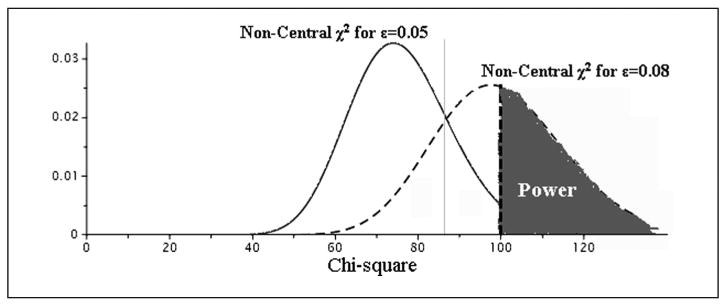
Estimation of the power using the noncentrality parameters of the χ² distribution for null and alternative hypothesis based on the RMSEA (root mean square error of approximation) values.

Figure 2.

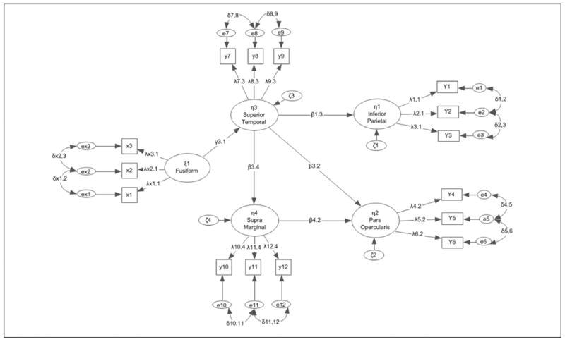
Hypothetical measurement model that formed the basis for the simulation using LISREL notation.

$$\lambda =(N-1)d{\varepsilon }^2$$ (2)

with N being the sample size, d the number of degrees of freedom, and ε² the null RMSEA₀ (the value of RMSEA that the model becomes acceptable). In the example of Figure 2, drawing a sample from Simos, Rezaie, Fletcher, and Papanicolaou (2013), the noncentrality parameter was estimated to be λ₀ = (ö− 1)dε² = (51 − 1) * 76 * (.05)² = 9.5 under the null hypothesis. The respective estimate for the alternative hypothesis λ₁ was (51 − 1) * 76 * (.08)² = 24.32. So, for approximate power of 80%, α = 5%, null RMSEA = .05, and a noncentrality parameter of 9.5, 159 participants would suffice. In this context, the present study examines how different sample sizes affect the behavior of the parameters in the model, namely, the omnibus chi-square test, Type I errors, and biased fit indices.

The Problem Under Study

Modeling neuroimaging data using SEM methods is challenging because it involves estimating a large number of parameters using relatively small sample sizes. This apparent contradiction is unfortunately built on our estimate of power estimation using the RMSEA: When the number of parameters is large (as in extended models that assess functional brain connectivity) the sample size required to evaluate close model fit, becomes increasingly small (Herzog, Boomsma, & Reinecke, 2007). For example, for a latent variable model with 80 indicators V defining 8 latent variables ξ, the required number of participants is 29! (for power equal to 80%, null RMSEA = .05 and alternative RMSEA = .02). It is rather utopic to expect that a sample size of 29 participants would suffice to measure population parameters (e.g., factor loadings, standard errors, etc.), for at least two reasons. First, the small sample size would adversely affect the estimate of the noncentrality parameter and thus, compromising the validity of the sample size estimation.³ Second, LRT estimates would likely reflect Type I errors, thus incorrect acceptance of poorly fitted models (Herzog & Boomsma, 2009). It has been well documented that chi-square tests are seriously inflated as the number of parameters increases (Herzog et al., 2007; Kenny & McCoach, 2003). Third, asymptotic distribution theory requires large numbers to provide stable estimates. MacCallum et al. (1996) suggested that N should always be greater than p. This proposition suggests that for a 70- or 80-item model, sample sizes of 71 or 81 participants would suffice. This, however, is a tentative assumption without strong support from the empirical literature. On the contrary, power analysis simulations most often suggest sample sizes greater than 200 participants (e.g., Cirillo & Barroso, 2012; Curran et al., 2003; Hu & Bentler, 1999) with 200 participants being particularly inadequate when model sizes increase (Herzog et al., 2007). Cases where smaller sample sizes have been recommended involve corrections of the maximum likelihood chi-square statistic for various factors (e.g., Bartlett, 1950; Swain, 1975; Yuan, 2005), which are beyond the scope of the present article. Table 1 presents sample size estimates for various SEM designs based on the noncentral chi-square test. As shown in Table 1, sample sizes range between 31 and 286 participants. In fact, designs having more than 20 measured indicators and between 4 and 10 latent variables, all required fewer than 100 participants. So a focal question relates to the adequacy of various sample sizes in latent variable structural models in order to explore functional connectivity in the brain.

Table 1.

Sample Sizes Required for Various Covariance Structure Models as a Function of RMSEA_diff Equal to .05 (i.e., RMSEA₀ = .05, RMSEA_a = .08).

Number of measured variables: Latent factors (ratio)	Sample size, N	Degrees of freedom, df
10:2	286	34
15:3	147	87
20:4	97	164
25:5	70	265
30:6	56	390
35:7	47	539
40:8	41	712
45:8	35	917
50:10	31	1130

Note. The degrees of freedom were estimated using the formula by Rigdon (1994), where df = m* (m+ 1)/2 − 2 *m−ξ* (ξ− 1)/2 − B −Γ. RMSEA = root mean square error of approximation.

Importance of the Study and Hypotheses Tested

At present the use of multivariate methods that account for the complexity and interactions in the brain are of limited use in applied research. Several methodologies have been proposed in the literature but have largely been inaccessible to applied researchers. Methods related to SEM have been proposed by Price et al. (2009) making use of Bayesian methods or Chen et al. (2011) suggesting autoregressive methods within path modeling but with measured variables rather than latent (see also Roebroeck, Formisano, & Goebel, 2005). One of the most prominent approaches to correlated structures involves the simplex model (Rogosa & Willett, 1985), which is traced originally to the pioneering work of Guttman (1954) and posits that later measures of a construct are regressed onto earlier measures of the same construct. It is important that proper methods are tested and made accessible so that the wealth of available neurophysiological information will be properly modeled. SEM is potentially one such methodology, as it allows for modeling complexities in behavior (e.g., model loops, cross-lagged effects, autocorrelation structures, etc.), given adequate sample sizes. Given cost-related issues in this line of research it is important to select a properly estimated sample size to achieve representativeness, parameter stability, and correct decision making (regarding hypotheses of model fit). Unfortunately, however, information about sample size cannot be drawn from other research-related power analyses as the specificity of the complex brain relationships needs to be properly modeled (e.g., by modeling multivariate relationships and autocorrelation structures). The use of earlier suggested rules of thumb cannot be relied on as these rules have been largely atheoretical (not model based), have been outdated, and are unable to account for the complexity often encountered with various data types (e.g., continuous versus categorical, dimensional, count, etc.). They are also silent with regard to model complexity, magnitude of communalities, missing data, and other factors. The present study attempts to (a) model a complex structure in the brain of typical readers and (b) evaluate the minimum sample size requirements to validly support the hypotheses of interest. The following research questions were examined:

1. What are the requirements in sample size to model an autoregressive structure in a confirmatory path model based on the RMSEA?

2. How do different sample sizes affect Type I errors of the LRT test?

3. How does sample size affect the behavior of various fit indices, when null hypotheses are true?

Method

Description of Study and Theoretical Model

The data in the present study came from Simos et al. (2013). Participants were 58 right-handed children (28 boys and 30 girls, with a mean age of 10.4 ± 1.6 years, range 7.5-12.5 years) with the valid cases being 51. Participants had never experienced difficulties in reading and scored >90 on the Basic Reading Composite (average of Word Attack and Letter-Word Identification subtest scores of the Woodcock–Johnson Tests of Achievement-III [W-J III]; Woodcock, McGrew, & Mather, 2001). Neuromagnetic activity was recorded from each student, while performing an oral reading task involving three-letter pronounceable nonwords (e.g., zan). Using a random schedule, four blocks of 25 stimuli were presented using a Sony LCD projector on a screen approximately 60 cm in front of each participant. Event-related magnetoencephalographic data segments were recorded with a whole-head neuromagnetometer array (4-D Neuroimaging, Magnes WH3600) time-locked to the onset of each stimulus. Following artifact rejection, low-pass filtering, baseline correction, and averaging across single epochs separately for each participant, a minimum norm algorithm was used to obtain estimates of the time-varying strength of intracranial currents (MNE Software, v. 2.5 http://www.nmr.mgh.harvard.edu/martinos/userInfo/data/index.php; Hämäläinen & Ilmoniemi, 1994) in approximately 6000 anatomically constrained cortical sources (obtained through a MRI-derived surface model of each participant's brain; Dale, Fischl, & Sereno, 1999). Temporally constrained pairwise functional associations between three left hemisphere temporoparietal regions (superior temporal gyrus, STG/BA22; supramarginal gyrus, SMG/BA40; angular gyrus, ANG/BA39), and the inferior frontal gyrus (IFG/BA44/45) were assessed. Functional contributions made by activity in the left fusiform gyrus (BA 37) to each of the temporoparietal regions and IFG were also explored (see Figure 2). The original study employed partial correlation analysis to evaluate pairwise interdependencies in the average current in successive 50-ms bins after controlling for autoregressive (or simplex model) effects. The latent variable model fitted to the same data is shown in Figure 2 as derived from the results of Simos et al. (2013) with two exceptions: paths from fusiform to the angular gyrus and from the angular gyrus to IFG were not associated with significant regression coefficients and were dropped from the model. The final structural model featured contributions by the left fusiform gyrus to the superior temporal gyrus, which in turn affected the degree of activity in the supramarginal, angular, and inferior frontal gyri. Activity in the inferior prefrontal cortex was determined by superior temporal and supramarginal activation (see Figure 2). Index variables defining each latent variable represented activity in early (150-200 ms after stimulus onset), middle (500-550 ms after stimulus onset), and late activation in each region (800-850 ms post–stimulus onset). The sample's estimates were used to simulate the data in the present study.

Covariance Structure Modeling: Description of the Model and the Simulation

The present model poses several challenges. First, it is multivariate in nature with several latent variables each defined by several indicators. Second, the indicators represent time series observations. Thus, a typical SEM structure would not hold. For this reason we tested a correlated structure that theoretically is described by an autoregressive process (in that observations at time t are a function of lagged variables from the preceding period; Curran & Bollen, 2001; van Buuren, 1997). Implementation of an autoregressive process on measured variables, rather than errors, was conducted as suggested by Chen et al. (2011) and J. Kim et al. (2007).

Estimating Power

Power analysis was conducted to estimate the required number of participants to achieve levels of power equal to 80% for the SEM model described in Figure 3. The estimation requires null and alternative models with regard to the magnitude of the RMSEA, the degrees of freedom, and the level of significance. The degrees of freedom were estimated by subtracting the number of model parameters (elements in the covariance matrix) from the number of free parameters in the model (factor loadings, variances of errors, and covariances). In SEM, the model parameters are equal to p(p + 1)/2, where p equals the number of measured variables [i.e., for a model with 70 measured variables, 70(70 + 1)/2 = 2485]. The number of free parameters equals the number of factor loadings, the errors and the factor covariances (in the above example they are equal to 161; 70 factor loadings, 70 errors, 21 factor covariances). The degrees of freedom for the structural model were estimated using the formula by Rigdon (1994): df = m* (m + 1)/2 − 2 *m−ξ* (ξ− 1)/2 − ö −Γ, with m being the number of measured variables, ξ the number of latent factors, and ö and Γ the number of coefficients that are estimated in the ö and Γ matrices. For the present study with a SEM model with 15 measured variables and 5 latent constructs, the number of degrees of freedom is 76 (i.e., 120 − 30 − 10 − 3 − 1). Power was estimated using the free package R (see Preacher & Coffman, 2006). For a sample syntax file, see the Appendix. The estimated sample size for a level of significance α = 5%, df = 76, null RMSEA₀ = .05 (which is a test of close fit) and an alternative RMSEA_a = .08 (test of not so close fit) equaled 159 participants. Thus, power analysis answered the question how many participants were required in order to rule out the hypothesis that two models with a difference of .03 points in their RMSEA values are significantly different from each other (difference between .05 and .08). The focal question of the present study was to evaluate sample sizes in which the power analysis estimate no longer holds.

Figure 3.

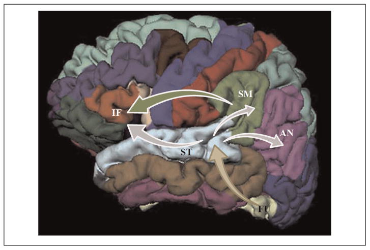
Schematic illustration of regional interdependencies included in the hypothetical measurement model assessed in the present study. According to this model the main source of input to the superior temporal gyrus (ST) originates in the fusiform gyrus (FU). Activity in the former region contributes directly to the activation observed in the supramarginal (SM), angular (AN; inferior parietal region in Figure 1), and inferior frontal gyri (IF; pars opercularis in Figure 1). A direct contribution from the supramarginal to the inferior frontal region is also included in the model.

Description of the Simulation

A Monte Carlo reactive simulation⁴ (Marcoulides & Saunders, 2006) was run with 1,000 samples being generated from the specified latent variable structural model of Figure 4). Sample sizes were increased by a unit of 10 for up to 100 participants and then following recommended conventions thus, there were samples of 20, 30, 40, 50, 60, 70, 80, 90, 100, 150, 200, 500, and 1,000 participants (Wolf et al., 2013). The samples of all sizes were generated from the original data of 51 students, using sampling with replacement (Simos et al., 2013). All analyses were run using the maximum likelihood estimation method and the factor loadings were modeled from the original data (Simulation 1) as well as a set of simulated data that posited all measurement and structural coefficients to have a standardized effect of .5 in order to evaluate power estimation with a configuration of modest relationships and thus, provide a blueprint for a wider range of measured relationships (Simulation 2). Autocorrelation coefficients were set as previously to .30. For the simulation that was guided from the original data, the standardized factor loadings guided the simulation were the following: For indicators X₁, X₂, and X₃, they were λ₁₁ = .652, λ₂₁ = .765, and λ₃₁ = .900; For items Y₁ to Y₁₂, they were λ₁₁ = .577, λ₂₁ = .769, λ₃₁ = .836, λ₄₁ = .915, λ₅₁ = .829, λ₆₁ = .636, λ₇₁ = .724, λ₈₁ = .737, λ₉₁ = .783, λ₁₀₁ = .659, λ₁₁₁ = .646, and λ₁₂₁ = .840. The structural paths were defined as follows: γ₃₁ = .874, β₁₃ = .977, β₃₂ = .867, and β₄₂ = .236. Lag-1 autocorrelation coefficients were fixed to .30 to provide for an identifiable effect given a medium effect size. Outcomes of interest were percentages of model solutions (out of 1,000) that converged, termed solution propriety (Gagne, & Hancock, 2006), mean significance estimate of chi-square tests, amount of Type I errors of the chi-square test, mean value of the RMSEA and minimum– maximum values, confidence intervals of the RMSEA, mean values of the measurement paths and minimum–maximum values, mean values of the structural paths and minimum–maximum values, and mean values of the following descriptive fit indices: goodness-of-fit index (GFI), AGFI, incremental fit index (IFI), McDonald fit index (MFI), NFI, nonnormed fit index (NNFI), and CFI. Bias, then, was evaluated as the difference between the simulated parameters and those of the sample (considered to be population parameters; Kelley & Maxwell, 2003) with values exceeding 5% of the population value being considered discrepant (Muthén & Muthén, 2002).

Figure 4.

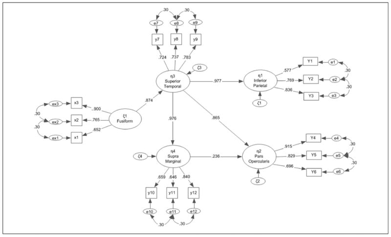
Measurement model with sample's parameter estimates that formed the basis for the first simulation study.

For all evaluations, reference model estimates were those obtained from simulation samples of 1,000 participants providing (through replacement) 1,000 replication samples. All subsequent comparisons were based on the above “population” model (e.g., difference in the estimates between the model having 50 participants versus the reference model with 1,000 participants across 1,000 simulations). Evidence in favor of the stability of parameters within a specific sample size would be provided when the following conditions were met (a) the RMSEA mean value should be contained within the confidence interval defining close fit (i.e., RMSEA < .05), (b) factor loading difference should be within recommended conventions (λ₁ − λ₂ < .10; Wang, Whittaker, & Beretvas, 2012), (c) Δ-Fit index variability should be within ±.02⁵ (Fan & Sivo, 2009), (d) more than 90% of the models should converge, and (e) Type I errors should be less than 25%.

Results

Power Analysis Based on the RMSEA and the Observed Sample Estimates (Simulation 1)

Table 2 summarizes the results for power levels equal to 80%. The second column refers to the average probability level observed on the chi-square test from 1,000 replications of size N. The third column refers to percentage of Type I errors again from 1,000 replications. The loading bias column (sixth column from the left) refers to the absolute discrepancy of the mean of the four structural paths (Figure 4) across the 1,000 replications. Last, for all estimates the reference model, characterized as the population model, was the model including sample sizes of 1,000 participants across 1,000 replications.

Table 2.

Simulation of Type I Errors, RMSEA Bias, Convergence, Factor Loading Bias, Structural Path Bias, and CFI Values as a Function of Number of Parameters and Sample Size Using 1,000 Replications: Simulation Is Based on Actual Data's Parameters.^a

Sample size, N	Mean probability of χ2	% of Type 1 errors based on χ2	Mean RMSEA	CI RMSEAb	Structural path mean bias Δc	Measurement path bias	CFI	% Model convergenced
20	.0106 (.000-.049)	95.1	.1740 (.114-.233)	.1135-.2194ncf	0.0422 (−0.077 to 0.084)	0.111 (−0.225 to 0.265)	.824 (.710-.926)	98.4
30	.0972 (.000-.464)	61.9	.0952 (.015-. 144)	.0383-.1427ncf	0.0559 (−0.084 to 0.011)	0.075 (−0.260 to 0.260)	.935 (.871-.998)	99.3
40	.1751 (.002-.634)	37.9	.0657 (.00-.110)	.0175-.1117ncf	0.0761 (−0.143 to 0.143)	0.062 (−0.119 to 0.251)	.966 (.920-1.000)	99.6
50	.2529 (.004-0.775)	25.2	.0479 (.000-.092)	.0098-.0924ncf	0.0081 (−0.002 to 0.013)	0.071 (−0.224 to 0.256)	.979 (.945-1.000)	99.9
60	.2964 (.006-.819)	20.4	.0383 (.000-.081)	.0067-.0807ncf	0.0079 (−0.006 to 0.016)	0.061 (−0.029 to 0.256)	.985 (.957-1.000)	99.9
70	.3059 (.009-.831)	20.4	.0345 (.000-.073)	.0059-.0741ncf	0.0057 (−0.003 to 0.009)	0.071 (−0.224 to 0.256)	.988 (.964-1.000)	100.0
80	.3379 (.010-.857)	15.2	.0293 (.000-.067)	.0043-.0672ncf	0.0035 (0.003 to 0.005)	0.071 (−0.223 to 0.256)	.991 (.972-1.000)	100.0
90	.3647 (.019-.866)	13.5	.0254 (.000-.059)	.0033-.0619ncf	0.0043 (−0.003 to 0.007)	0.071 (−0.223 to 0.257)	.993 (.977-1.000)	100.0
100	.3765 (.012-.883)	11.4	.0234 (.000-.059)	.0032-.0584ncf	0.00273 (−0.002 to 0.006)	0.071 (−0.224 to 0.257)	.993 (.977-1.000)	100.0
150	.4221 (.029-.916)	9.3	.0165 (.000-.044)	.0017-.0455cf	0.00298 (−0.001 to 0.005)	0.071 (−0.223 to 0.256)	.996 (.987-1.000)	100.0
200	.4351 (.030-.922)	8.3	.0136 (.000-.038)	.0014-.0389cf	0.00233 (−0.004 to 0.005)	0.071 (−0.224 to 0.257)	.997 (.990-1.000)	100.0
500	.4812 (.048-.939)	5.3	.0073 (.000-.022)	.0005-.0235cf	0.0017 (−0.003 to 0.003)	0.071 (−0.224 to 0.256)	.999 (.997-1.000)	100.0
1,000	.5028 (.049-.948)	5.1	.0048 (.00-.016)	.0004-.0162cf	Reference	0.071 (−0.223 to 0.257)	1.000 (.998-1.000)	100.0

Note. RMSEA = root mean square error of approximation; CFI = comparative fit index; CI = confidence interval.

^aValues in parentheses are minimum and maximum values of the relevant statistics.

^bncf = not close fit based on MacCallum et al. (1996); cf = close fit based on MacCallum et al. (1996).

^cEvaluated using a cutoff of 0.10 as an indication of a small bias (Wang et al., 2012).

^dN size required in order to identify a significant difference between two models that have a difference between .05 and .08 in RMSEA values. Percentage of models out of 1,000 simulations per sample size that converged without errors.

When looking at the mean RMSEA values, sample sizes of 50 participants were associated with mean RMSEA values less than .05, suggesting close fit. When considering the respective confidence intervals of RMSEA, sample sizes of approximately 70 participants were associated with models evaluating close and not so close fit 95% of the time. With 70 participants, the percentage of Type I errors of the chi-square was 20.4%, which represents a small margin of error for a test of exact fit (which is rather unrealistic). With 70 participants, 100% of the models converged, and the ΔCFI value suggested very small amounts of bias, equal to 0.012, less than the cutoff value of .02 suggested by Fan and Sivo (2009). Furthermore, the bias in the structural paths was negligible, that is, equal to 0.0057, and much less than the .10 criterion put forth by Wang et al. (2012). Thus, 70 participants would suffice to draw valid conclusions about a model having close to not so close fit across all standards and based on the actual sample's estimates.

A sample size of 50 participants was further associated with negligible path bias (equal to 0.0081) and plausible close fit according to mean RMSEA values. The vast majority of models converged properly (99.9% of the time) and the mean chi-square value was nonsignificant (for the strict test of exact fit). Thus, for liberal versus conservative estimates of sample size, 50 to 70 participants would be adequate in testing the hypothesized relationships of the model of Figure 3.

Sample sizes of 40 participants or less are not considered adequate as the upper level of the RMSEA confidence interval was above .10, which is indicative of a poorly fitted model. Interestingly, with 40 participants the structural paths bias was negligible thus stability of the parameters was not an issue. Furthermore, most models converged properly (99.6%).

For a test of close fit, one would need 150 participants in order for the RMSEA confidence interval to be less than .05 so that the value of close fit would be within the 95% confidence interval. This estimate is nevertheless, much lower than earlier recommendations regarding proper sample sizes. If, however, a researcher is targeting global fit measures, sizes of 150 participants are imperative.

When looking at the behavior of the fit indices, three were associated with minimum biases, less than .02, with sample sizes equal to 50 participants (see Figure 5). These were the CFI, the IFI, and the NNFI. The remaining indices were heavily influenced by sample size, which was expected given their formulae. Thus, these three indices suggested that sample sizes of 50 participants were associated with minimal bias and proper evaluation of model fit.

Figure 5.

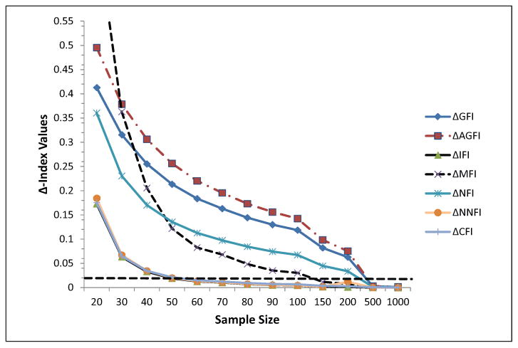
Δ-Index values as a function of sample size. The dashed line indicates a cutoff value of .02 as suggested by Fan and Sivo (2009). Estimates are based on simulating the responses from the Simos et al. (2013) functional magnetic resonance imaging study.

Power Analysis Based on the RMSEA and Parameter Estimates of Modest Magnitude (Simulation 2)

As a thoughtful reviewer stated the simulation based on the observed estimates from the Simos et al. (2013) study would underestimate sample sizes as model fit was excellent. Thus, the simulation was rerun with factor loading estimates equal to .5 in order to evaluate sample size needs with more realistic data sets. These findings are shown in Table 3 and Figure 6 for power levels equal to 80%. Results indicated that the findings from the second simulation closely replicated those from the observed data. Once again, sample sizes with 20 to 50 participants were associated with non-acceptable rejection rates of the chi-square statistic and corresponding power levels below .80. Thus, with regard to the omnibus chi-square test a sample size of 70 participants was associated 79.6% correct rejections. Similarly, if omnibus model fit is of interest, 150 participants would be required for the RMSEA value of 5% to be estimated within a 95% confidence interval. If, however, one is willing to accept a confidence interval window up to .08, which is still acceptable given conventional standards, a sample size of N = 60 would suffice. Of greater importance, however are parameter estimates and the ability to estimate them with minimal bias. Results, similar to the first simulation, indicated that again 50 participants suffice to accurately estimate measurement and structural paths or even smaller sample sizes; however, fewer than 50 participants were associated with worrisome effects on measures of global fit.

Table 3.

Simulation of Type 1 Errors, RMSEA Bias, Convergence, Factor Loading Bias, Structural Path bias, and CFI values as a Function of Number of Parameters and Sample Size Using 1,000 Replications: Simulation Is Based on Hypothetical Measurement and Structural Paths Equal to .50 in Order to Evaluate SEM Models With Moderate Fit.^a

Sample size, N	Mean probability of χ2	% of Type 1 errors based on χ2	Mean RMSEA	CI RMSEAb	Structural path mean bias Δc	Measurement path bias	CFI	% Model convergenced
20	.0113 (.000-.057)	94.1	.1742 (.111-.234)	.1135-.2197ncf	0.0987 (0.077-0.136)	0.0804 (−0.247 to 0.032)	.661 (.477-.845)	96.5
30	.1003 (.000-.478)	60.9	.0947 (.007-.145)	.0381-.1426ncf	0.0711 (−0.071 to 0.156)	0.0864 (−0.181 to 0.028)	.857 (.724-.999)	99.5
40	.178 (.001-.666)	38.7	.0655 (.000-.113)	.0178-.1116ncf	0.0766 (−0.096 to 0.132)	0.0797 (−0.154 to 0.0158)	.921 (.820-1.000)	99.3
50	.2516 (.003-785)	24.5	.0480 (.000-.093)	.0096-.0926ncf	0.0731 (0.035 to 0.115)	0.0744 (−0.215 to 0.006)	.950 (.871-1.000)	100.0
60	.297 (.008-.812)	21.0	.0385 (.000-.080)	.0070-.0809ncf	0.0847 (−0.121 to 0.176)	0.0764 (−0.186 to 0.020)	.964 (.896-1.000)	99.8
70	.3055 (.008-.826)	20.4	.0348 (.000-.074)	.0060-.0740ncf	0.0665 (0.025 to 0.106)	0.0728 (−0.213 to 0.006)	.970 (.916-1.000)	100.0
80	.3399 (.010-.857)	15.8	.0292 (.000-.067)	.0044-.0671ncf	0.0659 (0.028 to 0.107)	0.0722 (−0.211 to 0.005)	.977 (.930-1.000)	100.0
90	.3612 (.014-.872)	13.5	.0257 (.000-.061)	.0035-.0623ncf	0.0632 (0.027 to 0.103)	0.0717 (−0.210 to 0.007)	.982 (.943-1.000)	100.0
100	.3797 (.012-.887)	13.2	.0233 (.000-.059)	.0035-.0584ncf	0.0609 (0.022 to 0.104)	0.0714 (−0.208 to 0.007)	.984 (.943-1.000)	100.0
150	.4213 (.030-.921)	8.4	.0164 (.000-.044)	.0015-.0454cf	0.0616 (0.022 to 0.105)	0.0698 (−0.205 to 0.006)	.991 (.969-1.000)	100.0
200	.4300 (.031-.920)	8.3	.0138 (.000-.037)	.0013-.0390cf	0.0574 (0.016 to 0.105)	0.0697 (−0.206 to 0.007)	.994 (.977-1.000)	100.0
500	.4824 (.053-.942)	4.7	.0072 (.000-.022)	.0004-.0235cf	0.0555 (0.013 to 0.098)	0.0714 (−0.202 to 0.008)	.998 (.992-1.000)	100.0
1,000	.5014 (.049-.942)	5.2	.0048 (.000-.016)	.0004-.0162cf	Reference	0.0683 (−0.203 to 0.008)	.999 (.996-1.000)	100.0

Note. RMSEA = root mean square error of approximation; CFI = comparative fit index; SEM, structural equation modeling; CI = confidence interval.

^aValues in parentheses are minimum and maximum values of the relevant statistics.

^bncf = not close fit based on MacCallum et al. (1996); cf = close fit based on MacCallum et al. (1996).

^cEvaluated using a cutoff of 0.10 as an indication of a small bias (Wang et al., 2012).

^dN size required in order to identify a significant difference between two models that have a difference between .05 and .08 in RMSEA values. Percentage of models out of 1,000 simulations per sample size that converged without errors.

Figure 6.

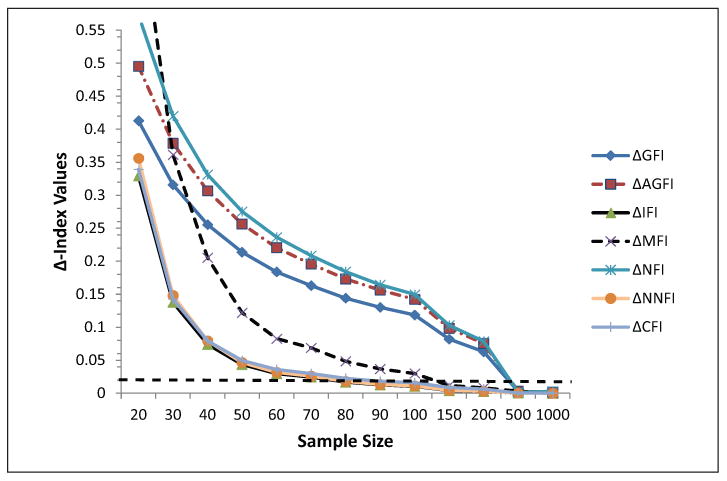
Δ-Index values as a function of sample size. The dashed line indicates a cutoff value of .02 as suggested by Fan and Sivo (2009). Data are based on the simulated data with measurement and structural paths equal to .500.

Fit indices became substantially worse compared with the original data simulation (see Figure 6). That is, previously sample sizes of 50 participants were associated with minimal bias when relying on the CFI, IFI, and NNFI. When simulating factor loadings to have modest contributions to the latent construct, the required sample sizes for bias less than .02 shifted from 50 participants to 80 participants. Thus, with regard to those three descriptive fit indices, required sample sizes are greater than 80 participants or between 70 and 80 participants. With 150 participants, the MFI was also within a minimum margin of error; all other fit indices, however, required more than 500 participants, which is likely prohibitive for this line of research.

Discussion and Conclusions

The present study attempted to evaluate the minimum sample size requirements to validly support specific hypotheses regarding functional brain connectivity using real neuromagnetic data. The results showed that 50 to 70 participants seemed to suffice in order to maintain low Type-I error rates, ensure RMSEA values are between .05 and .08 and stable model parameters. Models converged properly (convergence ranged between 99.9% and 100% for sample sizes equal or greater than 50 participants). Estimates of change in descriptive fit statistics were also below the cutoff point of 0.02 with just 50 participants given the simulation that relied on actual data and between 70 and 80 participants using more modest parameter effects. These estimates are much lower compared to earlier recommendations of sample sizes in structural equation modeling (e.g., MacCallum et al., 1996; MacCallum & Hong, 1997) and are much larger compared to estimates proposed with regard to path models (Chen et al., 2011; Price et al., 2009), or longitudinal latent variable models. These findings are encouraging for researchers modeling brain relationships as they recommend manageable numbers.

Modeling the above relations with 40 participants seemed to be unacceptable because the error rates of the chi-square test increase exponentially. The RMSEA was between close and not so close fit but with a larger confidence interval that moved beyond acceptance. The loading bias for both measurement and structural paths was also worrisome. Thus, as earlier researchers did before us we do not recommend the use of sample sizes with fewer than 40 participants (e.g., Chin, & Newstead, 1999; Muthén & Muthén, 2002). Thus, this sample size is not sufficient. The marginal size of 50 participants was associated with a properly accepting chi-square test but with a Type I error of 25%. The point estimate of the RMSEA was acceptable but not its confidence interval that just went higher than .08. Thus 60 to 70 participants are needed to ensure proper model fit and decision making. The above recommendation is based on simulating the actual data set; when using more modest parameter estimates the required sample size becomes N = 80.

One advantage of the present study relates to modeling and simulation of real functional connectivity data, thus, distributional issues and idiosyncrasies of such data were properly accounted for and this analysis was also supplemented with a simulation having more modest effects in order to provide suggestions based on a broader range of estimated models (i.e., having more modest relationships. This contrasts with previous simulation studies using fixed factor loadings that may not resemble real relationships and actual estimates of measurement error. Also, this study captures the essential limitation of observing a large amount of Type I errors of the chi-square test with data that misfit a model (E. S. Kim, Yoon, & Lee, 2012). Moreover, the correlated nature of brain connectivity was modeled using novel auto-regressive methods suggested by J. Kim et al. (2007) by first evaluating the observed lagged relationships. Thus, the findings of the present simulation likely reflect real rather than artificial scenarios of hypothesized regional brain interdependencies. Another advantage of the present study was that a manageable number of indicators was selected (based on lagged relationships) so that conservative estimates of power were obtained (large numbers of indicators could result in excessive power estimates; Marsh, Hau, Balla, & Grayson, 1998; Wolf et al., 2013).

Interestingly, we did not find as great as an effect of the magnitude of factor loadings and their influence on sample size as previous researchers (Wolf et al., 2013). For example, we concluded that 70 participants would be adequate for both global model fit and stability of item parameters with the simulation of observed data (that had strong measurement and structural relations). When modeling modest relations, however, we found that only a marginal increase in sample size (from 70 to 80 participants) was required to observe both proper model fit and stable parameter estimates. Under various conditions Wolf et al. (2013) recommended between 60 and 190 observations.

Researchers should also target the largest sample size possible to improve proximity with population parameters (Kelley & Maxwell, 2003). Additionally, power should be estimated for the smallest-needed estimated effect. For example, if the interest is in deciphering a small-to-medium correlation between two activation areas, then large samples would be needed and one would need to estimate power for that specific configuration.

The present study is limited by a number of factors. First, the analysis was not performed for power levels equal to .90 or .95 (see Wang et al., 2012). Such power levels would be associated with findings that would require much larger samples. Instead, the present findings reflect the absolute minimum in terms of sample size requirements and should be viewed as conservative, and in light of contributing absolutely minimum recommendations to the applied researcher. Second, the model tested was of medium size involving only five brain regions and three time indicators per region so inferences about larger models cannot be made. However, such a restricted model is much more appropriate to estimate measurement error in assessing activity in brain areas through latent variables, compared to aggregated terms. Third, the present power estimates are based on real data and thus, the first simulation's findings are bound to the specificities and idiosyncrasies of the present sample and magnetoence-phalography data set. It is important to state here, however, that even larger effects with regard to reading behavior in dyslexia have been previously reported (Koyama et al., 2013). To account for that limitation we conducted an ancillary proactive simulation in order to evaluate the requirements of minimum sample size with more modest effects (i.e., factor loadings and structural paths equal to .50 in standardized values). Fourth, a number of factors that influence the present estimates have not been accounted for. For example, nonnormality in the data or various missing patterns can seriously moderate the present findings (Davey & Salva, 2009). Fifth, there must be a mention of the positive bias of RMSEA in conditions when it is estimated to be below zero (Curran et al., 2003; Fan, Thompson, & Wang, 1999). Last, the present simulation presents sample size estimation using a specific approach, which has its own limitations (Herzog & Boomsma, 2009), and assumptions (Curran et al., 2002) although other alternatives to sample size estimation exist (e.g., Muthén & Muthén, 2002; Satorra & Saris, 1985).

In the future, it will be interesting to estimate factors related to the reliability of the measured constructs and ways to account for low reliability when modeling the hypothesized relationships. For example, if constructs are defined by lagged effects one may consider including a large number of lagged relationships (Bollen & Curran, 2004) in order to improve construct reliability (Wolf et al., 2013). Also, it will be interesting to see where the power analysis model breaks down as the number of parameters increases for a given sample size or when the data misfit the model. The issue of sample size estimation for multigroup models may become particularly important as one would want to test various configurations in the brain across groups (Raykov, Marcoulides, Lee, & Chang, 2013). Regardless, the present study suggests that a modest and realistic number of participants suffices to model complex, time-dependent interrelationships in regional brain activity.

Appendix

R routine for the estimation of power as a function of a difference between .05 and .08 in the RMSEA, for a 50-item, 5-factor scale (the syntax came from Preacher & Coffman, 2006). Power for the estimated model below was equal to 80%.

alpha <- 0.05 ! Define alpha level relevant to the study; it is for a two-tailed test

d <- 1165 ! Provide the estimated degrees of freedom of the model for which power is estimated

n <- 31 ! Provide the number of participants for which power is estimated

rmsea0 <- 0.05 ! Provide null RMSEA value

rmseaa <- 0.08 ! Provide alternative RMSEA value

ncp0 <- (n-1)*d*rmsea0ˆ2

ncpa <- (n-1)*d*rmseaaˆ2

if(rmsea0<rmseaa) {

cval <- qchisq(alpha,d,ncp=ncp0,lower.tail=F)

pow <- pchisq(cval,d,ncp=ncpa,lower.tail=F)

}

if(rmsea0>rmseaa) {

cval <- qchisq(1-alpha,d,ncp=ncp0,lower.tail=F)

pow <- 1-pchisq(cval,d,ncp=ncpa,lower.tail=F)

}

print(pow)! Printing of results on screen

References

- Bartlett MS. Tests of significance in factor analysis. British Journal of Psychology. 1950;3:77–85. [Google Scholar]
- Bentler PM, Chou CH. Practical issues in structural equation modeling. Sociological Methods & Research. 1987;16:78–117. [Google Scholar]
- Bollen KA. An alternative two stage least squares (2SLS) estimator for latent variable equations. Psychometrika. 1996;61:109–121. [Google Scholar]
- Bollen KA, Curran PJ. Autoregressive latent trajectory (ALT)models: A synthesis of two traditions. Sociological Methods & Research. 2004;32:336–383. [Google Scholar]
- Boomsma A. Robustness of Lisrel against small sample sizes in factor analysis models. In: Jöreskog KG, Wold H, editors. Systems under indirection observation: Causality, structure, prediction (Part I) Amsterdam, Netherlands: North Holland: 1982. pp. 149–173. [Google Scholar]
- Breivik E, Olsson U. Adding variables to improve fit: The effect of model size on fit assessment in Lisrel. In: Cudeck R, du Toit S, Sorbom D, editors. Structural equation modeling: Present and future. Lincolnwood, IL: Scientific Software International; 2001. pp. 169–194. [Google Scholar]
- Browne MW, Cudeck R. Alternative ways of assessing model fit. In: Bollen KA, Long JS, editors. Testing structural equation models. Newbury Park, CA: Sage; 1993. pp. 136–162. [Google Scholar]
- Chen G, Glen DR, Saad ZS, Paul Hamilton J, Thomason ME, Gotlib IH, Cox RW. Vector autoregression, structural equation modeling, and their synthesis in neuroimaging data analysis. Computers in Biology and Medicine. 2011;41:1142–1155. doi: 10.1016/j.compbiomed.2011.09.004. [DOI] [PMC free article] [PubMed] [Google Scholar]
- Cheung GW, Rensvold RB. Evaluating goodness-of-fit indexes for testing measurement invariance. Structural Equation Modeling. 2002;9:233–255. [Google Scholar]
- Chin W, Newstead P. Structural equation modeling analysis with small samples using partial least squares. In: Hoyle R, editor. Statistical strategies for small sample research. Thousand Oaks, CA: Sage; 1999. pp. 307–341. [Google Scholar]
- Cirillo MA, Barroso LP. Robust regression estimates in the prediction of latent variables in structural equation models. Journal of Modern Applied Statistical Methods. 2012;11:42–53. [Google Scholar]
- Curran PJ, Bollen KA. The best of both worlds: Combining autoregressive and latent curve models. In: Collins LM, Sayer AG, editors. New methods for the analysis of change. Washington, DC: American Psychological Association; 2001. pp. 105–136. [Google Scholar]
- Curran PJ, Bollen KA, Chen F, Paxton P, Kirby J. Finite sampling properties of the point estimates and confidence intervals of the RMSEA. Sociological Methods & Research. 2003;32:208–252. [Google Scholar]
- Curran PJ, Bollen KA, Paxton P, Kirby J, Chen F. The noncentral chi-square distribution in misspecified structural equation models: Finite sample results from a Monte Carlo simulation. Multivariate Behavioral Research. 2002;37:1–36. doi: 10.1207/S15327906MBR3701_01. [DOI] [PubMed] [Google Scholar]
- Dale AM, Fischl B, Sereno MI. Cortical surface-based analysis. I. Segmentation and surface reconstruction. NeuroImage. 1999;9:179–194. doi: 10.1006/nimg.1998.0395. [DOI] [PubMed] [Google Scholar]
- Davey A, Salva J. Estimating statistical power with incomplete data. Organizational Research Methods. 2009;12:320–346. [Google Scholar]
- Fan X, Sivo SA. Using Δgoodness-of-fit indexes in assessing mean structure invariance. Structural Equation Modeling. 2009;16:54–69. [Google Scholar]
- Fan X, Thompson B, Wang L. Effects of sample size, estimation method, and model specification on structural equation modeling fit indexes. Structural Equation Modeling. 1999;6:56–83. [Google Scholar]
- Gagne P, Hancock G. Measurement model quality, sample size, and solution propriety in confirmatory factor models. Multivariate Behavioral Research. 2006;41:65–83. doi: 10.1207/s15327906mbr4101_5. [DOI] [PubMed] [Google Scholar]
- Guttman LA. A new approach to factor analysis. The radix. In: Lazarsfeld PF, editor. Mathematical thinking in the social sciences. New York, NY: Columbia University Press; 1954. pp. 258–348. [Google Scholar]
- Hancock GR, Freeman MJ. Power and sample sizes for the root mean square error of approximation test of not close fit in structural equation modeling. Educational and Psychological Measurement. 2001;61:741–758. [Google Scholar]
- Hämäläinen MS, Ilmoniemi RJ. Interpreting magnetic fields of the brain: Minimum norm estimates. Medical and Biological Engineering and Computing. 1994;32:35–42. doi: 10.1007/BF02512476. [DOI] [PubMed] [Google Scholar]
- Herzog W, Boomsma A. Small-sample robust estimators of noncentrality-based and incremental model fit. Structural Equation Modeling. 2009;16:1–27. [Google Scholar]
- Herzog W, Boomsma A, Reinecke S. The model-size effect on traditional and modified tests of covariance structures. Structural Equation Modeling. 2007;14:361–390. [Google Scholar]
- Hu LT, Bentler PM. Cutoff criteria for fit indexes in covariance structure analysis: Conventional criteria versus new alternatives. Structural Equation Modeling. 1999;6:1–55. [Google Scholar]
- Iacobucci D. Structural equation modeling: Fit indices, sample size, and advanced topics. Journal of Consumer Psychology. 2010;20:90–98. [Google Scholar]
- Jung S. Structural equation modeling with small sample sizes using two-stage least-squares estimation. Behavior Research Methods. 2013;45:75–81. doi: 10.3758/s13428-012-0206-0. [DOI] [PubMed] [Google Scholar]
- Kelley K, Maxwell SE. Sample size for multiple regression: Obtaining regression coefficients that are accurate, not simply significant. Psychological Methods. 2003;8:305–321. doi: 10.1037/1082-989X.8.3.305. [DOI] [PubMed] [Google Scholar]
- Kenny DA, McCoach DB. Effect of the number of variables on measures of fit in structural equation modeling. Structural Equation Modeling. 2003;10:333–351. [Google Scholar]
- Kim ES, Yoon M, Lee T. Testing measurement invariance using MIMIC: Likelihood ratio test with a critical value adjustment. Educational and Psychological Measurement. 2012;72:469–492. [Google Scholar]
- Kim J, Zhu W, Chang L, Bentler PM, Ernst T. Unified structural equation modeling approach for the analysis of multisubject, multivariate functional MRI data. Human Brain Mapping. 2007;28:85–93. doi: 10.1002/hbm.20259. [DOI] [PMC free article] [PubMed] [Google Scholar]
- Koyama M, Martino A, Kelly C, Jutagir D, Sunshine J, Schwartz S, Milham M. Cortical signatures of dyslexia and remediation: An intrinsic functional connectivity approach. PLoS One. 2013;8(2):e55454. doi: 10.1371/journal.pone.0055454. [DOI] [PMC free article] [PubMed] [Google Scholar]
- Loehlin JC. Latent variable models: An introduction to factor, path, and structural equation analysis. Mahwah, NJ: Lawrence Erlbaum; 2004. [Google Scholar]
- MacCallum RC, Browne MW, Sugawara HM. Power analysis and determination of sample size for covariance structure modeling. Psychological Methods. 1996;1:130–149. [Google Scholar]
- MacCallum RC, Hong S. Power analysis in covariance structure modeling using GFI and AGFI. Multivariate Behavioral Research. 1997;32:193–210. doi: 10.1207/s15327906mbr3202_5. [DOI] [PubMed] [Google Scholar]
- MacCallum RC, Lee T, Browne MW. The issue of isopower in power analysis for tests of structural equation models. Structural Equation Modeling. 2010;17:23–41. [Google Scholar]
- Marcoulides GA. Structural equation modeling for scientific research. Journal of Business and Society. 1989;2:130–138. [Google Scholar]
- Marcoulides GA. Evaluation of confirmatory factor analytic and structural equation models using goodness-of-fit indices. Psychological Reports. 1990;67:669–670. [Google Scholar]
- Marcoulides GA, Saunders C. PLS: A silver bullet? MIS Quarterly. 2006;30:iii–ix. [Google Scholar]
- Marsh H, Balla J, McDonald R. Goodness of fit indices in confirmatory factor analysis. Psychological Bulletin. 1988;103:391–410. [Google Scholar]
- Marsh H, Hau KT, Balla JR, Grayson D. Is more ever too much? The number of indicators per factor in confirmatory factor analysis. Multivariate Behavioral Research. 1998;33:181–220. doi: 10.1207/s15327906mbr3302_1. [DOI] [PubMed] [Google Scholar]
- McQuitty S. Statistical power and structural equation models in business research. Journal of Business Research. 2004;57:175–183. [Google Scholar]
- Meade AW, Johnson EC, Braddy PW. The utility of alternative fit indices in tests of measurement invariance; Paper presented at the annual Academy of Management Conference; Atlanta, GA. 2006. Aug, [Google Scholar]
- Muthén LK, Muthén BO. How to use a Monte Carlo study to decide on sample size and determine power. Structural Equation Modeling. 2002;4:599–620. [Google Scholar]
- Nunnally JC. Psychometric theory. New York, NY: McGraw-Hill; 1967. [Google Scholar]
- Olsson UH, Foss T, Troye SV, Howell RD. The performance of ML, GLS, and WLS estimation in structural equation modeling under conditions of misspecification and nonnormality. Structural Equation Modeling. 2000;7:557–595. [Google Scholar]
- Preacher KJ, Coffman DL. Computing power and minimum sample size for RMSEA. 2006 [Computer software]. Available from http://quantpsy.org/
- Price LR, Laird AR, Fox PT, Ingham RJ. Modeling dynamic functional neuroimaging data using structural equation modeling. Structural Equation Modeling. 2009;16:147–162. doi: 10.1080/10705510802561402. [DOI] [PMC free article] [PubMed] [Google Scholar]
- Raykov T. On the large sample bias, variance, and mean squared error of the conventional noncentrality parameter estimator of covariance structure models. Structural Equation Modeling. 2000;7:431–441. [Google Scholar]
- Raykov T, Marcoulides GA. Multivariate effect size estimation: confidence interval construction via latent modeling. Journal of Educational and Behavioral Statistics. 2010;35:407–421. [Google Scholar]
- Raykov T, Marcoulides GA, Lee CL, Chang C. Studying differential item functioning via latent variable modeling: A note on a multiple-testing procedure. Educational and Psychological Measurement. 2013;73:898–908. [Google Scholar]
- Rigdon EE. Calculating degrees of freedom for a structural equation model. Structural Equation Modeling. 1994;1:274–278. [Google Scholar]
- Roebroeck A, Formisano E, Goebel F. Mapping directed influence over the brain using granger causality mapping. NeuroImage. 2005;25:230–242. doi: 10.1016/j.neuroimage.2004.11.017. [DOI] [PubMed] [Google Scholar]
- Rogosa D, Willett J. Satisfying a simplex structure is simpler than it should be. Journal of Educational Statistics. 1985;10:99–107. [Google Scholar]
- Rottelo C, Zeng M. Analysis of RT distributions in the remember-know paradigm. Psychonomic Bulletin & Review. 2008;15:825–832. doi: 10.3758/pbr.15.4.825. [DOI] [PubMed] [Google Scholar]
- Satorra A, Saris WE. Power of the likelihood ratio test in covariance structure analysis. Psychometrika. 1985;50:83–90. [Google Scholar]
- Simos PG, Rezaie R, Fletcher JM, Papanicolaou AC. Time-constrained functional connectivity analysis of cortical networks underlying phonological decoding in typically developing school-aged children: A magnetoencephalography study. Brain & Language. 2013;125:156–164. doi: 10.1016/j.bandl.2012.07.003. [DOI] [PMC free article] [PubMed] [Google Scholar]
- Steiger JH. Structural model evaluation and modification: An interval estimation approach. Multivariate Behavioral Research. 1990;25:173–180. doi: 10.1207/s15327906mbr2502_4. [DOI] [PubMed] [Google Scholar]
- Steiger JH, Lind JM. Statistically based tests for the number of common factors; Paper presented at the annual meeting of the Psychometric Society; Iowa City, IA. 1980. Jun, [Google Scholar]
- Swain AJ. Unpublished doctoral dissertation. Department of Statistics, University of Adelaide; Australia: 1975. Analysis of parametric structures for variance matrices. [Google Scholar]
- van Buuren S. Fitting ARMA time series by structural equation models. Psychometrika. 1997;62:215–236. [Google Scholar]
- Wang D, Whittaker T, Beretvas N. The impact of violating factor scaling method assumptions on latent mean difference testing in structured means models. Journal of Modern Applied Statistical Methods. 2012;11:24–41. [Google Scholar]
- Wolf E, Harrington KM, Clark SL, Miller MW. Sample size requirements for structural equation models: An evaluation of power, bias, and solution propriety. Educational and Psychological Measurement. 2013;73:913–934. doi: 10.1177/0013164413495237. [DOI] [PMC free article] [PubMed] [Google Scholar]
- Woodcock RW, McGrew KS, Mather N. Woodcock-Johnson III Tests of Achievement. Itasca, IL: Riverside; 2001. [Google Scholar]
- Yuan KH. Fit indices versus test statistics. Multivariate Behavioral Research. 2005;40:115–148. doi: 10.1207/s15327906mbr4001_5. [DOI] [PubMed] [Google Scholar]