Shape Mode Analysis Exposes Movement Patterns in Biology: Flagella and Flatworms as Case Studies

Abstract

We illustrate shape mode analysis as a simple, yet powerful technique to concisely describe complex biological shapes and their dynamics. We characterize undulatory bending waves of beating flagella and reconstruct a limit cycle of flagellar oscillations, paying particular attention to the periodicity of angular data. As a second example, we analyze non-convex boundary outlines of gliding flatworms, which allows us to expose stereotypic body postures that can be related to two different locomotion mechanisms. Further, shape mode analysis based on principal component analysis allows to discriminate different flatworm species, despite large motion-associated shape variability. Thus, complex shape dynamics is characterized by a small number of shape scores that change in time. We present this method using descriptive examples, explaining abstract mathematics in a graphic way.

Introduction

Life presents itself in manifold morphologies. Quantifying morphology is often the first step to relate form and function. A common task in shape characterization amounts to finding those morphological features and geometric quantities with maximal descriptive power. This is especially challenging when aiming to understand shape changes of soft or flexible structures, such as beating cilia or animals without rigid skeletons. Shape mode analysis is a standardized way to find such quantities a posterori, after data collection, by combining a large number of partially redundant morphometric features into a small set of distinct shape scores [1]–[5].

Shape mode analysis is a well-known technique in engineering and computer science, e.g. for image recognition [6], yet only recently researchers began to apply it to biological data sets. One of the earliest application of this method to biological shape data was by Sanger et al., analyzing human arm posture [7]. Pioneered by Ryu et al., shape mode analysis has been particularly used to analyze motility patterns of the round worm C. elegans [3], [8]–[10].

Here, we adapt principal component analysis to analyze and quantify movement patterns in two 2D image data sets: (i) the bend centerline of beating flagella, and (ii) the closed boundary outline of gliding flatworms. We reconstruct a limit cycle of flagellar oscillations using a data set from swimming bull sperm, which allows us to study not only regular flagellar oscillations, but also noisy deviations from perfect periodicity, thereby contributing to the characterization of the flagellum as a noisy oscillator [11], [12].

In contrast to flagella or the slender shapes of the round worm C. elegans, many cells and organisms display morphologies that are more suitably described by their outline contour. However, outline contours can vary dramatically in the absence of skeletal elements, as is the case in planarian flatworms. Planarians have recently become an important model system for regeneration and growth dynamics [13]. Their flattened and elongated body plan morphology is kept in shape by a deformable extracellular matrix material and the contraction status of their muscular plexus. Many species exist worldwide that often differ in body shape. However, measuring body shape in behaving animals is challenging, because changes in muscle tone constantly change the projected body shape and still images therefore rarely capture the “true” shape of the animal. Accurate quantification of shape in fixed specimens is similarly problematic, owing to various contraction artifacts of the fixation methods. We therefore thought to explore shape mode analysis with respect to its utility in extracting average shape information from movie sequences of living animals. As a first test, we analyzed an extensive high-precision tracking data set of gliding flatworms. Planarians display a smooth gliding motility, resulting from the coordinated beat patterns of the cilia in their densely ciliated ventral epithelium [14], [15]. We find that a bending mode correlates with active turning during gliding motility, showing that steering is achieved by a bending of the long body axis. Additional modes characterize stereotypic width changes of these worms not reported before. These width changes are shown to become particularly pronounced during a second type of motility behavior, inch-worming, normally associated to escape responses, but also observed in phenotypes with impaired cilia functionality [14], [15]. Our method reveals regular lateral contraction waves with a period of about in inch-worming worms. We find that the extraction of body postures from tracked outline contours enables accurate shape measurements of flatworms, which we demonstrate by the ability to differentiate between different flatworm species. Supporting the notoriously difficult taxonomy of these soft-bodied animals with statistical quantification of genus- or species specific body shapes represents an interesting application of our method.

By analyzing two typical classes of biological data sets in a pedagogical setting and by explaining the mathematics in a graphic way, we hope to provide an accessible account of this versatile method. Here, shape mode analysis is based on the mathematical technique of principal component analysis and allows to project a multi-feature data set on a small set of empirical shape modes, which are directly inferred from the data itself. Principal component analysis thus represents a dimensionality-reduction technique, where a big data set residing in a high-dimensional ‘feature space’, is projected from onto a convenient ‘shape space’ of lower dimension with minimal information loss [4], [5]. As a side-effect, this method reduces measurement noise by averaging over several, partially redundant features. The wide applicability of principal component analysis comes at the price of a diverse terminology across different disciplines, see Table 1.

Table 1. Principal component analysis is used across different disciplines, giving rise to a diverse terminology, which is summarized here.

			Ref.
coefficients, loadings	principal components	eigenvalues	[4]
characteristic vectors, eigenvectors	z-scores	characteristic roots, latent roots	[5]
eigenvectors	amplitudes	eigenvalues	[8]
coefficients, loadings	scores	latents, eigenvalues	MATLAB [43]

For simplicity, we focus on linear principal component analysis in the main text. In an appendix, we discuss non-linear generalizations such as kernel methods and show how these can be used to analyze angular data, using the sperm data set as a descriptive example. Our analysis demonstrates how to relate organism shape and motility patterns in a pedagogical setting using flagella and flatworms as prototypical examples.

Results and Discussion

A minimal example

First, we discuss a minimal example to illustrate the key concept of dimensionality reduction by principal component analysis, which forms the basis of our shape mode analysis approach.

Assume we are given a data set that comprises geometrical features measured for each of individuals, say the distribution of length and height in a shoal of fish such that , see Fig. 1A. To mimic the partial redundancy of geometrical features commonly observed in real data, we further assume that these two features are strongly correlated, see Fig. 1B.

Figure 1. Illustration of principal component analysis.

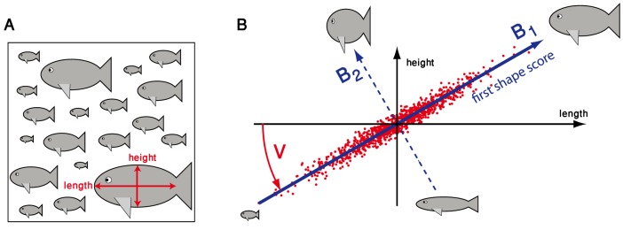
A. As a minimal example, we consider a hypothetical data set of length and height measurements for a collection of individuals, i.e. there are just geometric features measured here. B. In this example, length and height are assumed to be strongly correlated, thus mimicking the partial redundancy of geometrical features commonly observed in real data. Principal component analysis now defines a change of coordinate system from the original (length,height)-axes (shown in a black) to a new set of axes (blue) that represent the principal axes of the feature-feature covariance matrix of the data. Briefly, the first new axis points in the direction of maximal data variability, while the second new axis points in the direction of minimal data variability. The change of coordinate system is indicated by a rotation around the center of the point cloud representing the data. By projecting the data on those axes that correspond to maximal feature-feature covariance, in this example the first axis, one can reduce the dimensionality of the data space, while retaining most of the variability of the data. In the context of morphology analysis, we will refer to these new axes as ‘shape modes’ , which represent specific combinations of features. The new coordinates are referred to as ‘shape scores’ .

Principal component analysis now defines a unique change of coordinate system such that the new axes (blue) point along the principal directions of feature-feature covariance: in the new coordinate system, the shape coordinates become linearly uncorrelated. In the context of shape mode analysis, the new axes are called ‘shape modes’ , while the corresponding coordinates will be referred to as ‘shape scores’ . The first shape mode points into the direction of maximal variation in the data. In this example, the shape score corresponding to this first shape mode provides a robust measure of size that combines length and height measurements. The remaining second shape mode points along the direction of least covariance. The corresponding shape score can be interpreted as an aspect ratio in this example. As this second shape score displays only little variation, the data set is well described by just the first shape score , which represents an effective dimensionality reduction from to one dimension.

We emphasize that the concept of an measurement-feature matrix is rather generic and is encountered in many other contexts, such as measurements of dynamic flagellar centerline shapes or flatworm outlines as discussed next.

Characterizing the flagellar beat as a biological oscillator

Sperm cells are propelled in a liquid by regular bending waves of their flagellum, a slender cell appendage of length [16]. The flagellar beat is powered by ten-thousands of dynein molecular motors inside the flagellum that constantly convert chemical energy into mechanical work [17]. The regular shape changes of the flagellum determine speed and direction of sperm swimming [18], [19]. Eukaryotic flagella propel also many other microswimmers including green algae and ciliated Protozoans, or participate in fluid transport inside multicellular animals [20]. Here, we analyze a data set of flagellar swimming of bull sperm [21] using shape mode analysis. Methods are described in [21]; the frame-rate was .

Tangent angles characterize flagellar waves

In these experiments, sperm cells swam parallel to a boundary surface with an approximately planar flagellar beat. This effective confinement to two space dimension greatly facilitates tracking of flagellar shapes and their analysis. The (projected) shape of a bent flagellum at a time is described by the position vector of points along the centerline of the flagellum for , where is the arclength along the flagellar centerline and the total flagellar length, see Fig. 2A. To characterize shapes, we need a description that is independent of the actual position and orientation of the cell in space. To this end, we introduce a material frame of the sperm head consisting of the head center position and a unit vector pointing along the long axis of the prolate sperm head. The length of this long axis is , such that corresponds to the proximal tip of the flagellum. Additionally, we introduce a second unit vector , which is obtained by rotating in the plane of swimming by an angle of in a counter-clockwise fashion. With respect to this material frame, the tracked flagellar shape is characterized by a tangent angle as [19], [21]

(1)

Figure 2. Principal shape modes of sperm flagellar beating.

A. High-precision tracking of planar flagellar centerline shapes (, red) are characterized by their tangent angle as a function of arc-length along the flagellum. B. The time-evolution of this flagellar tangent angle is shown as a kymograph. The periodicity of the flagellar beat is reflected by the regular stripe patterns in this kymograph; the slope of these stripes is related to the propagation of bending waves along the flagellum from base to tip. By averaging over the time-dimension, we define a mean flagellar shape characterized by a tangent angle profile . For illustration, this mean flagellar shape is shown in black superimposed to tracked flagellar shapes (grey). C. We define a feature-feature covariance matrix from the centered tangent angle data matrix as explained in the text. The negative correlation at arc-length distance reflects the half-wavelength of the flagellar bending waves. D. The normalized eigenvalue spectrum of the covariance matrix sharply drops after the second eigenvalue, implying that the eigenvectors corresponding to the first two eigenvalues together account for 97% of the observed variance in the tangent angle data. E. Using principal component analysis, we define two principal shape modes (blue, red), which correspond precisely to the two maximal eigenvalues of the covariance matrix in panel C. The lower plot shows the reconstruction of a tracked flagellar shape (black) by a superposition of the mean flagellar shape and these two principal shape modes (magenta). In addition to tangent angle profiles, respective flagellar shapes are shown on the right. F. Each tracked flagellar shape can now be assigned a pair of shape scores and , indicating the relative weight of the two principal shape modes in reconstruction this shape. This defines a two-dimensional abstract shape space. A sequence of shapes corresponds to a point cloud in this shape space. We find that these point form a closed loop, reflecting the periodicity of the flagellar beat. We can define a shape limit cycle by fitting a curve to the point cloud. By projecting the shape points on this shape limit cycle, we can assign a unique flagellar phase modulo to each shape. This procedure amounts to a binning of flagellar shapes according to shape similarity. G. By requiring that the phase variable should change continuously, we obtain a representation of the beating flagellum as a phase oscillator. The flagellar phase increases at a rate equal to the frequency of the flagellar beat and rectifies the progression through subsequent beat cycles by increasing by . H. Amplitude fluctuations of flagellar beating as a function of flagellar phase. An instantaneous amplitude of the flagellar beat is defined as the radial distance of a point in the -shape space, normalized by the radial distance of the corresponding point on the limit cycle of same phase. A phase-dependent standard deviation was fitted to the data (black solid line). Also shown are fits for additional cells (gray; the position of was defined using a common set of shape modes). J. Swimming path of the head center during one beat cycle computed for the flagellar wave given by the shape limit cycle (panel F) using resistive force theory [18] as described previously [19]. The path is characterized by a wiggling motion of the head superimposed to net propulsion. For a ‘standing wave’ beat pattern characterized by the oscillation of only one shape mode, net propulsion vanishes.

This tangent angle measures the angle between the vector and the local tangent of the flagellum at position . Importantly, this tangent angle representation characterizes flagellar shape independent of cell position and orientation. Tracking a high-speed recording with frames corresponding to time-points and using control points along the flagellum, we obtain an measurement matrix for the tangent angle with . This matrix represents a kymograph of the flagellar beat; an example is shown in Fig. 2B. The apparent stripe pattern reflects the periodicity of the flagellar beat. The slope of the stripes is directly related to the wave velocity of traveling bending waves that pass down the flagellum from its proximal to its distal end. On a more abstract level, the matrix comprises independent measurements (time points) of geometric features (tangent angle at the control points).

PCA decomposition of flagellar bending waves

We will now show how a set of principal shape modes can be extracted from this representation. First, we define a mean shape of the flagellum by averaging each column of the matrix , i.e. we average over the measurements [21]. The resultant mean tangent angle and corresponding flagellar shape is shown in Fig. 2B. We note that taking a linear mean of angular data is admissible here, since angles stay in a bounded interval and do not jump by ; a general procedure that can cope also with jumps of is discussed in the appendix. The mean tangent angle is non-zero, which relates to an intrinsic asymmetry of the flagellar bending waves. Asymmetric flagellar beating implies swimming along curved paths [19], [22]. Cellular signaling can change this flagellar asymmetry [23] and has been assigned a crucial role in non-mammalian sperm chemotaxis [24]. Here, we are interested in flagellar shape changes, i.e. deviations from the mean shape. Thus, we devise an -matrix all of which rows are equal to the mean tangent angle . We can now compute the feature-feature covariance matrix as

(2)

see Fig. 2C. We find strong positive correlation along the main diagonal of this covariance matrix (dashed line), which implies that tangent angle measurements at nearby control points are correlated. This short-range correlation relates to the bending stiffness of the flagellum. It implies partial redundancy among the measurements corresponding to nearby control points along the flagellum. More interestingly, we find negative correlation between the respective tangent angles that are an arclength distance apart. What does this mean? The flagellar beat can be approximated as a traveling bending wave with a certain wave length . This wavelength manifests itself as a “long-range correlation” in the covariance matrix .

We will now employ an eigenvalue decomposition of the covariance matrix C, yielding eigenvalues and eigenvectors such that . In analogy to the minimal example above, we refer to the eigenvectors as shape modes. The shape modes correspond to axes of a new coordinate system of feature space; in this coordinate system, the variations of the data along each axis are linearly uncorrelated and have respective variance for axis , . We can assume without loss of generality that the eigenvalues of are sorted in descending order, see Fig. 2D. For the sperm data, we observe that the eigenvalue spectrum sharply drops after ; in fact, the first two shape modes and together account for of the variance of the data. We now choose to deliberately chop the eigenvalue spectrum after and project the data set on the reduced “shape space” spanned by the shape modes and . Generally, the mode-number cutoff will be application specific and requires supervision. Formal criteria to chose the optimal cutoff have been discussed in the literature, see e.g. [2] and references therein.

Each recorded flagellar shape, that is each row of the data matrix can now be uniquely expressed as a linear combination of the shape modes

(3)

The shape scores can be computed by a linear least-square fit. Fig. 2E displays the principal shape modes and as well as the superposition of a typical flagellar shape into these two modes. Using this procedure, the entire data set gets projected onto an abstract shape space with just two axes representing the shape scores and .

Limit cycle reconstruction

Inspecting Fig. 2F, we find that the shape point cloud in shape space forms a closed loop: During each beat cycle, the shape points corresponding to subsequent flagellar shapes follow this shape circle to make one full turn. Thus, the shape space representation reflects the periodicity of the flagellar beat [25]. As a next step, we can fit a closed curve to this point cloud, which defines a “shape limit cycle”. We can then project each point of the cloud onto this limit cycle; this assignment is indicated as color-code in Fig. 2F. We parameterize the shape limit cycle by a phase angle that advances by after completing a full cycle. Furthermore, one can always assume that this phase angle increases uniformly along the curve [26]. This procedure assigns a unique phase to each tracked flagellar shape and is equivalent to a binning of flagellar shapes according to shape similarity. We have thus arrived at a description of periodic flagellar beating in terms of a single phase variable that increases continuously

(4)

where is the angular frequency of flagellar beating, see Fig. 2G. Eq. (4) is a phase oscillator equation, which is a popular theoretical description for generic oscillators. This minimal description represents a starting point for more elaborate descriptions. For example, external forces have been shown to speed up or slow down the flagellar beat, which can be described by a single extra term in equation (4) [25]. Further, the scatter of the shape point cloud around the limit cycle of perfectly periodic flagellar beating reflects active fluctuations of the flagellar beat, which can be analyzed in a similar manner [11].

As an application of the shape-space representation, we follow [11] to define an instantaneous amplitude of the flagellar beat as the radial distance of a point in the -shape space, normalized by the radial distance of the corresponding point on the limit cycle of same phase. We find that the fluctuations of this amplitude are phase-dependent, attaining minimal values during bend initiation at the proximal part of the flagellum, see Fig. 2H. We argue that these amplitude fluctuations represent active fluctuations stemming from the active motor dynamics inside the flagellum that drives flagellar waves. As a test for the contribution from measurement noise, we added random perturbations to the tracking data, using known accuracies of tracking [21]. Phases and amplitudes computed for perturbed and unperturbed data were strongly correlated.

In conclusion, the reduction of the full data set comprising feature dimensions to just a single phase variable involved a linear dimension reduction using principal component analysis to identify a shape limit cycle, followed by a problem-specific non-linear dimensionality reduction, the projection onto this limit cycle, to define phase and amplitude. In future work, the shape space representation of the flagellar beat developed here can be used to quantify responses of the flagellar beat to mechanical or chemical stimuli.

Undulatory swimming with two shape modes

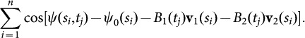
We will close this section by relating the results of our shape analysis to the hydrodynamics of flagellar swimming. For simplicity, we neglect variations of the flagellar beat and consider a perfect flagellar bending wave characterized by a “shape point” circling along the “shape limit cycle”. At the length scale of a sperm cell, inertia is negligible and the hydrodynamics of sperm swimming is governed by a low Reynolds number, which implies peculiar symmetries of the governing hydrodynamic equation (the Stokes equation) [27]. In particular, the net displacement of the cell after one beat cycle will be independent of how fast the “shape limit cycle” is transversed. Further, playing the swimming stroke backwards in time would result exactly in a reversal of the motion. This implies that no net propulsion is possible for a reciprocal swimming stroke that looks alike when played forward or backward [28]. The periodic modulation of just one shape mode is an example of such a reciprocal swimming stroke. In fact, the periodic modulation of one shape mode represents a standing wave, which does not allow for net propulsion, but implies that the sperm cells transverses a closed loop during a beat cycle, see Fig. 2J. The superposition of two shape modes, however, represents a minimal system for swimming: the superposition of two standing waves results in a traveling wave that breaks time-reversal symmetry and thus allows for net propulsion. The relation between standing and traveling waves can be illustrated by a minimal example of a trigonometric identity, which decomposes a traveling wave on the l.h.s. into two, periodically modulated shape modes of sinusoidal shape

(5)

In this minimal example, the shape modes would be given by sinusoidal standing wave profiles and with oscillating shape scores given by and . Here, corresponds to the wave-length of the waves. In the limit of small beat amplitudes, it can be formally shown that the net swimming speed of the cell is proportional to the area enclosed by the shape limit circle [29].

Shape and motility analysis of flatworms

We now apply shape mode analysis to time-lapse imaging data of the flatworm Schmidtea mediterranea (Fig. 3A). This animal is a popular model organism for studies on regeneration and growth [13]. Flatworms (greek: Platyhelminthes) represent some of the simplest organisms with bilateral body plan. Yet, they possess a distinct brain with two lobes, setting them apart from simpler worms like C. elegans. Flatworms can steer their path in response to light, chemical stimuli, and temperature. Even a limited ability for learning has been proposed, including habituation and Pavlovian conditioning [30]. Hence, flatworms posses a sufficiently rich behavioral repertoire, whose control mechanisms are unknown to date. Flatworms are found in virtually all parts of the world, living in both salt- and freshwater, and include parasitic species like the cause of bilharzia. A subset of non-parasitic species, commonly referred to as ‘planarians’, with Schmidtea mediterranea as a prominent member, is now entering the stage of modern model organisms to study regeneration, growth, and associated motility phenotypes [13], [31].

Figure 3. Three shape modes characterize projected flatworm body shape dynamics.

A. Our custom-made MATLAB software tracks worms in movies and extracts worm boundary outline (red) and centerline (blue). B. The radial distance between the boundary points and midpoint of the centerline (, red dot) is calculated as a parameterization of worm shape. We normalize the radial distance profile of each worm by the mean radius . C. The second symmetry axis (dotted line) of the covariance matrix corresponds to statistically symmetric behavior of the worm with respect to its midline. D. The three shape modes with the largest eigenvalues account for 94% of the shape variations. The first shape mode characterizes bending of the worm and alone accounts for 61% of the observed shape variance. On the top, we show its normalized radial profile on the left as well as the boundary outline corresponding to the superposition of the mean worm shape and this first shape mode (solid red: , dashed red: , black: mean shape with ). The second shape mode describe lateral thinning (), while the third shape mode corresponds unlike deformations of head and tail (), giving the worm a wedge-shaped appearance. E. The first shape mode with score describing worm bending strongly correlates with the instantaneous turning rate of worm midpoint trajectories. F. We manually selected 30 movies where worms clearly show inch-worming and 50 movies with no inch-worming behavior. The variance of score and increases for the inch-worming worms. G. The autocorrelation of mode and the crosscorrelation between mode and mode reveals an inch-worming frequency of approximately , hinting at generic behavioral patterns.

Unlike the roundworm C. elegans, planarians do not move by undulatory body motion. Instead, planarians glide over the substratum, being propelled by the beating of numerous short flagella (or cilia) that project from their multi-ciliated ventral epithelium. Planaria lack a rigid body wall and thus possess comparably soft bodies that can deform significantly by muscle contractions. Thus, a continuous challenge in the field is the development of a reliable method to quantify shape variations of these soft-bodies animals. Below, we characterize their pronounced shape plasticity using shape mode analysis to characterize the outline of two-dimensional projections of their flat body. Similar characterization of outlines as closed curves are likely to be encountered in other contexts, such as the shape analysis of adherent or crawling cells [32].

Worm handling and tracking

In the experiments, we use a clonal line of an asexual strain of Schmidtea mediterranea [33], [34]. Worms were maintained at 20°C as described in [35] and were starved for at least one week prior to imaging. To monitor the 2D-projection of the worm body as in Fig. 3A, we used a Nikon macroscope (AZ 100M, 0.5x objective) and a Nikon camera set-up (DS-Fi1, frame rate 3 Hz, total observation period 15 s, resolution 1280×960 pixel). The flatworms were placed one at a time into a plastic petri dish ( mm), clean petri dishes were used for each experimental series (comprising movies of worms). After being exposed to light, worms displayed a typical flight response. Movies were analyzed off-line using custom-made MATLAB software. A first shape proxy was determined from background-corrected movie frames via edge detection using a canny-filter, followed by a dilation-erosion cycle. In a subsequent refinement step, the worm perimeter was adjusted by finding the steepest drop in intensity along directions transverse to the perimeter proxy. As a result we were able to automatically track the boundary outline (red) as well as the centerline (blue) of worms with sub-pixel accuracy in a very robust manner, see Fig. 3A.

Radial profiles characterize non-convex outlines

In analyzing the tracked outline shapes, we face the challenge of characterizing the shape of closed, planar curves. For non-convex shapes, this can be non-trivial. We describe a closed curve by a position vector as a function of arc-length along its circumference, see Fig. 3B. We use the tip of the worm tail as a distinguished reference point that specifies the position of . We further specify a center point , using the midpoint of the tracked centerline of the worms. The profile of radial distances measured with respect to the center point characterizes outline shape, even for non-convex outlines. Shapes of convex curves might also be characterized by a profile of radial distances as a function of a polar angle . However, this definition does not generalize to non-convex curves (or, more precisely, to curves that are not radially convex with respect to ). To adjust for different worm sizes, we normalize the radial distance profiles by the mean radius as and plot it as a function of normalized arc-length , where is the total length of the circumference. As a mathematical side-note, we remark that using the signed curvature along the circumference, instead of the radial distance profile , would amount to a significant disadvantage: The property that a certain curvature profile actually corresponds to a closed curve imposes a non-trivial constraint on the set of admissible curvature profiles. For the normalized radial distance profiles, however, there is a continuous range of distance profiles that correspond to closed curves, making this choice of definition more suitable for applying linear decomposition techniques such as shape mode analysis. In fact, given a particular normalized radial distance profile, the corresponding circumference length is reconstructed self-consistently by the requirement that the associated curve must close on itself.

A bending mode and two width-changing modes

We extracted worm outlines from a total of 745 analyzed movies. We computed normalized radial distance profiles as described above, each profile being represented by radii, resulting in a large data matrix. From the average of all radial profiles, we define a mean worm shape that averages out shape variations, see Fig. 3D (right inset,black). Next, we computed the covariance matrix between the individual radial profiles, using the centered (mean-corrected) data matrix, Fig. 3C. The symmetry of the covariance matrix along the dotted diagonal shows that shape variations are statistically symmetric with respect to the worm midline. Again, the eigenvectors corresponding to the largest eigenvalues of this matrix are those with maximal descriptive power for shape variance. Fig. 3D shows the first three shape modes, which together account for of the observed shape variance. We find that the dominant shape mode is anti-symmetric, describing an overall bending of the worm. In contrast, the second and third mode describe symmetric width changes of the worm: The second shape mode characterizes a lateral thinning of the worm associated with a pointy head and tail. Correspondingly, a negative contribution of the second shape mode with describes lateral thickening of the worm (with slightly more roundish head and tail). The third shape mode , finally, is also symmetric and is associated with unlike deformations of head and tail, giving the worm a wedge-like appearance. Superpositions of these three shape modes describe in-plane bending of the worms, and a complex width dynamics of head and tail.

The bending mode characterizes turning

Next, we investigated the relationship between flatworm shape and motility. Flatworms employ numerous beating cilia on their ventral epithelium to glide on surfaces. We observe that worms actively regulate their gliding speed over a considerable range of , in quantitative agreement with earlier work [36]. Yet, we did not observe pronounced correlations between shape dynamics and gliding speed (not shown). This is consistent with the notion that muscle contractions play a minor role in the generation of normal gliding motility. However, we find that shape changes control the direction of gliding motility and thus steer the worm's path: Fig. 3E displays a significant correlation between the rate of turning along the worm trajectory and the first shape score , which characterizes bending of the worm. The sign and magnitude of this “bending score” directly relates to the direction and rate of turning. For simplicity, we had restricted the analysis to a medium size range of 8–10 mm length, analogous results are found for other size ranges.

The second and third modes characterize inch-worming

In addition to cilia-driven gliding motility, flatworms employ a second, cilia-independent motility pattern known as inch-worming, which provides a back-up motility system in case of dysfunctional cilia [14] or as an escape response. To test whether modes two and three might relate to this second motility pattern, we analyzed movies of small worms known to engage more frequently in this kind of behaviour.

We therefore manually classified movies of worms smaller than mm that have been starved for 10 weeks, yielding a number inch-worming and non-inch-worming worms for a differentiated motility analysis (cases of ambiguity were not included). We find that the second and third shape mode, which characterize dynamic variations in body width, are indeed more pronounced in inch-worming worms, see Fig. 3F. Next, we computed the temporal autocorrelation of time series of the second shape mode , see Fig. 3G (solid blue). We observe stereotypical shape oscillations with a characteristic frequency of 0.26 Hz. From the cross-correlation between and in Fig. 3G (dashed black), we find that both shape scores oscillate with a common frequency and relative phase lag of (where lags behind). Thus, both shape modes act together in an orchestrated manner to faciliate inch-worming, hinting at coordinated muscle movements and periodic neuronal activity patterns.

In conclusion, we identified different shape modes that can characterize different fundamental types of motility in a quantitative manner. The characteristic periodic shape dynamics associated with inch-worming posses the question about underlying generic patterns of neuronal and muscular activity.

PCA discriminates flatworm species

Having developed tools to measure shape changes of the same animal over time, we next explored the utility of shape mode analysis in shape comparisons between different animals. The model species Schmidtea mediterranea is but one of many hundred flatworm species existing worldwide [37]. The taxonomic identification of planarian species is challenging, relying largely on the time-consuming mapping of internal characters. The availability of quantitative bodyplan morphological parameters would be of interest in this context. Having available a large live collection of planarian species, we choose four species representing the genera Girardia, Phagocata, Schmidtea and Polycelis. Besides potentially size-dependent variations in aspect ratio, the four species differ by their characteristic head shapes, see Fig. 4A. Accordingly, we restricted shape analysis to the head region only (defined as the most anterior of the worm body). We characterized each head shape by a vector of distances from the midpoint of the head (red dot, of the worm length from the tip of the head) to the outline of the head region and proceeded as above. We found that the first two eigenmodes captured of head shape variability within this multi-species data set. Fig. 4B shows species-specific mean shapes for each of the four species in a combined head shape space, as well as ellipses of variance covering (dark color) and (light color) of motility-associated shape variability, respectively. This comparison of flatworm species representing four genera illustrates linear dimensionality reduction as a simple means to map morphological differences across species.

Figure 4. Distinguishing head morphologies of four different flatworm species.

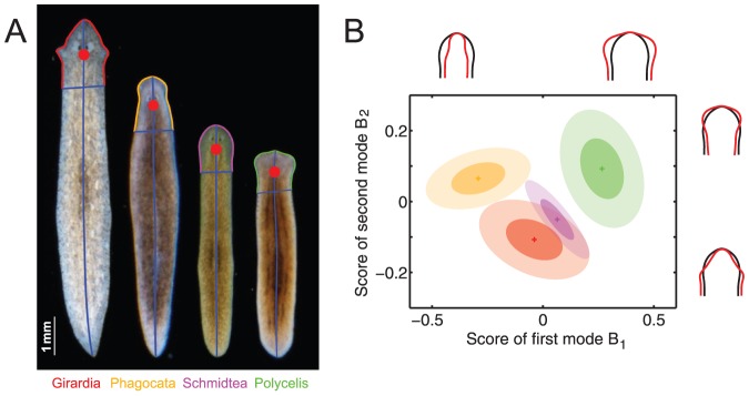
A. Application of our method to parametrize head morphology of four different flatworm species. For each species, time-lapse sequences of different worms were recorded as two independent runs of duration frames. The head is defined as most anterior of the worm body. Radial distances are computed with respect to the midpoint of the head (red dot at of the worm length from the tip of the head). B. By applying PCA to this multi-species data set, we obtain two shape modes, which together account for of the shape variability. Deformations of the mean shape with respect to the the two modes are shown (black: mean shape, red: superposition of mean shape and first mode with and second mode with , respectively). We represent head morphology of the four species in a combined shape space of these two modes. Average head shapes for each species are indicated by crosses, with ellipses of variance including (dark color) and (light color) of motility-associated shape variability, respectively.

Conclusion

Using two biological examples, swimming sperm and gliding flatworms, we demonstrated shape mode analysis as a versatile tool to characterize morphological shapes and its dynamical changes. In both cases, we obtained a low-dimensional description of organism shape. Our observation that complex shapes dynamics can be concisely described by just a few shape scores corroborates the high coordination of molecular motor activity in the sperm flagellum, as well as contraction of muscles in flatworms during both gliding and inch-worming motility, respectively.

In the case of a beating flagellum, shape mode analysis revealed a limit cycle that characterizes the periodicity of the beat. This limit cycle allowed the definition of a flagellar phase that rectifies the progression through a periodic sequence of shapes as well as the quantification of noisy deviations from perfectly periodic shape dynamics. In the appendix, we comment on the challenges to deal with the periodicity of angular data.

In the case of flatworms, shape mode analysis concisely characterizes a behavioral repertoire and the associated body shape dynamics. It is known that flatworms employ two distinct motility mechanisms: (i) gliding motility, relying on beating of their ventral cilia with occasional turns, and, (ii) inch-worming, which is driven by muscle contractions [14], [15]. We find that bending and turning maneuvers are strongly correlated, revealing a generic mechanism for steering. Furthermore, we quantitatively analyzed the motility mechanisms of inch-worming, which is evoked in case of dysfunctional cilia [14], [15] or as an escape response. We observe a concerted shape dynamics of lateral thinning of head and tail with a characteristic period of about . Our analysis can serve as basis for future studies of generic behavioral responses in planarians and underlying patterns of neuronal and muscular activity, irrespective of their higher level of complexity [3], [8] compared to other model organisms such as C. elegans. Previous studies of planarian motility had focused on coarse-grained motility parameters such as net speed or the mean-squared-displacement of worm tracks [36]. To the best of our knowledge, our study represents the first application of shape mode analysis to flatworm motility, linking shape and motion in a quantitative manner, thus enabling the characterization of motility phenotypes.

Additionally, our method presents a simple means to compare and distinguish different flatworm species. Further refinements of the method that take into account the whole body shape could generate a useful supplement of taxonomic traits to help in the classification of new planarian species. Further, the ability to precisely quantify differences in head shape now enable the dissection of the underlying molecular pathways that control morphogenesis. Based on the principal components defining head shape, it is conceivable that planarian head morphogenesis is mainly controlled by two molecular networks: One controlling maximal head width at the position of the auricles and a second one determining the posterior displacement of the point of maximal head width. The availability of transcriptome sequence information for these species (Liu et al, in preparation) will now allow testing of this hypothesis, e.g., by RNAi screens with shape mode analysis as read-out or systematic expression level comparisons in head transcriptomes of species with different head morphologies. Similar inter-species comparisons of beak morphology in Darwin finches could be correlated with the ecological niche of the animals [38]. The corners of the observed shape set corresponded to archetypical species that are highly specialized to a narrow environmental niche, while species corresponding to interior points of the shape set represent generalists, whose fitness is optimized simultaneously for several traits. It will be interesting to test similar hypotheses for flatworm species, some of which inhabit extreme environments.

Mathematical appendix: PCA for angular data and kernel methods

We discuss an extension of principal component analysis using a distance kernel, which is particularly suited for the analysis of angular data. Linear operations on angular data can be problematic, e.g. if angles jump by . We define a feature-feature similarity matrix that accounts for the -ambiguity of angle data

(6)

Rows and columns of this matrix do not automatically average to zero, so kernel centering [39] has to be applied,

We can now proceed as below eq. (2), obtaining shape modes from the eigenvectors of the matrix . (Without kernel centering, the resultant shape modes would comprise a contribution from the non-zero average of all the measurements [40].) Shape scores can be defined by maximizing the similarity measure

Here, the ‘mean flagellar shape’ is defined using the circular mean . Fig. 5 compares the first shape mode and its scores for this kernel PCA and linear PCA as considered in the main text.

Figure 5. Principal component analysis for angular data using kernel PCA.

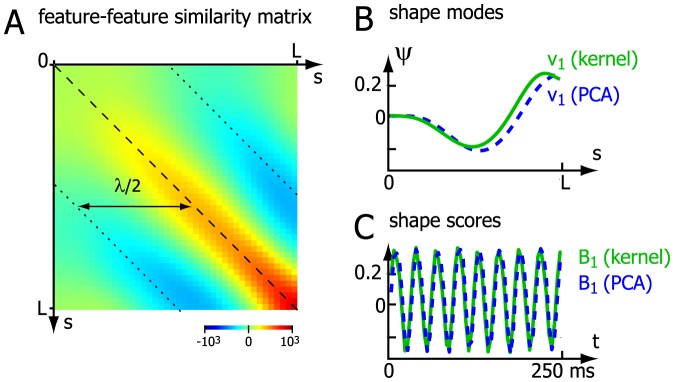
A. Centered feature-feature similarity matrix according to eq. (6) for the sperm tangent angle data. B. First shape mode for the kernel method (green) compared to the first shape mode as obtained by linear PCA (blue dashed). C. Corresponding shape scores as a function of measurement time for both the kernel method (green) and for linear PCA (blue dashed).

If one is only interested in shape scores, but not the corresponding shape modes, an alternative approach would be to use a measurement-measurement similarity matrix

known as a Gram's matrix [39]. The eigenvalues and eigenvectors , , of the kernel-centered Gram matrix provide a proxy for the shape scores via .

A mathematical motivation for the use of such kernel methods stems from the fact eq. (2) can be interpreted as a special case of a similarity kernel. For linear PCA, the eigenvector decomposition of the feature-feature covariance matrix and that of the measurement-measurement covariance matrix yield analogous results as can be shown using the singular value decomposition of the mean centered data matrix

(7)

Here, and are unitary and matrices, respectively, and is a diagonal matrix. From eq. (7), we readily fi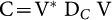nd and , where and are diagonal matrices with the same eigenvalues. These matrix decompositions are illustrated in Fig. 6 for linear PCA on sperm data.

Figure 6. The mathematics behind principal component analysis (PCA).

A. For illustration, we start with a measurement matrix featuring the beat of a sperm flagellum with measurement (rows) and tangent angles at equidistant positions along the flagellar centerline (columns). Subtracting the mean defines the centered data matrix . The mathematical technique of singular value decomposition factors the data matrix into a product of a unitary matrix , a “diagonal” matrix that has non-zero entries only along its diagonal, and a unitary matrix . Singular value decomposition may be regarded as a generalization of the usual eigensystem decomposition of symmetric square matrices to non-square matrices. A unitary matrix U generalizes the concept of a rotation matrix to n-dimensional space.; it is defined by being equal to the identity matrix. Second row: A restriction to the top- singular values defines sub-matrices of , , of dimensions , , , respectively, whose product represents a useful approximation of the full factorization that reduces feature dimensions to only shape modes. B. The feature-feature covariance matrix is defined in terms of the centered data matrix . It can be written as a product of a diagonal matrix , whose diagonal features the eigenvalues of and a unitary -matrix V whose columns correspond to the respective (left) eigenvectors of . This matrix V is exactly the same as previously encountered in the singular value decomposition of . C. Similarly, the measurement-measurement covariance matrix , known as the Gram matrix, can be decomposed using a diagonal matrix and a unitary matrix . Importantly, the rows of V comprise just the shape modes of the data matrix as defined by linear PCA, while the columns of the matrix yield the corresponding shape scores.

Using a nonlinear similarity measure as in eq. (6) breaks the exact correspondence between PCA and kernel PCA based on the measurement-measurement covariance matrix. Nevertheless, the use of kernels allows to analyze more complicated data sets and depicts the road to nonlinear dimension reduction methods [39]. In fact, several nonlinear dimensionality reduction algorithms rely on kernel PCA, including the popular Isomap algorithm [41]. Such algorithms have been used for automated frame-sorting, including flagellar video-microscopy [42]. Additionally, the concept of a Gram matrix is used in multi-dimensional-scaling to reconstruct embeddings into a high-dimensional feature space using only a Gram matrix of mutual distances between individual measurements.

Supporting Online Material

A Matlab script is a available for download that illustrates the method of shape mode analysis by principal component analysis, and the reconstruction of a limit cycle as shown in Fig. 2.

Supporting Information

File S1

Example source code (Matlab) demonstrating the use of PCA and limit cycle reconstruction, closely following the analysis of sperm tracking data shown in Fig. 2 . The reader is invited to study this code interactively. First, a pseudo data set is generated, thereby making the program independent of any data files. Then, principal component analysis is applied and shape modes and scores are displayed. A limit cycle is fitted to the resulting shape space dynamics, and the uniform phase parametrization is derived. Finally, singular value decomposition and kernel PCA are visualized.

(M)

Data Availability

The authors confirm that all data underlying the findings are fully available without restriction. All relevant data are within the paper.

Funding Statement

SW and BMF received funding from the BMBF grant 031 A 099 (http://www.bmbf.de/en/1398.php). The funders had no role in study design, data collection and analysis, decision to publish, or preparation of the manuscript.

References

- 1.Pearson K (1901) On lines and planes of closest fit to systems of points in space. The London, Edinburgh, and Dublin Philosophical...: 559–572.
- 2. Abdi H, Williams LJ (2010) Principal component analysis. Wiley Interdisciplinary Reviews: Computational Statistics 2:433–459. [Google Scholar]
- 3. Stephens GJ, Johnson-Kerner B, Bialek W, Ryu WS (2010) From modes to movement in the behavior of Caenorhabditis elegans. PloS one 5:e13914. [DOI] [PMC free article] [PubMed] [Google Scholar]
- 4.Jolliffe I (2005) Principal component analysis. Wiley Online Library.
- 5.Jackson JE (2005) A user's guide to principal components. John Wiley & Sons.
- 6. Cootes T, Taylor C, Cooper D, Graham J (1995) Active Shape Models-Their Training and Application. Computer Vision and Image Understanding 61:38–59. [Google Scholar]
- 7. Sanger TD (2000) Human arm movements described by a low-dimensional superposition of principal components. The Journal of neuroscience: the official journal of the Society for Neuroscience 20:1066–72. [DOI] [PMC free article] [PubMed] [Google Scholar]
- 8. Stephens GJ, Johnson-Kerner B, Bialek W, Ryu WS (2008) Dimensionality and dynamics in the behavior of C. elegans. PLoS Comp Biol 4:e1000028. [DOI] [PMC free article] [PubMed] [Google Scholar]
- 9. Raviv TR, Ljosa V, Conery AL, Ausubel FM, Carpenter AE, et al. (2010) Morphology-guided graph search for untangling objects: C. elegans analysis. Medical image computing and computer-assisted intervention: MICCAI International Conference on Medical Image Computing and Computer-Assisted Intervention 13:634–41. [DOI] [PMC free article] [PubMed] [Google Scholar]
- 10. Gallagher T, Bjorness T, Greene R, You YJ, Avery L (2013) The geometry of locomotive behavioral states in C. elegans. PloS one 8:e59865. [DOI] [PMC free article] [PubMed] [Google Scholar]
- 11. Ma R, Klindt GS, Riedel-Kruse IH, Jülicher F, Friedrich BM (2014) Active Phase and Amplitude Fluctuations of Flagellar Beating. Physical Review Letters 113:048101. [DOI] [PubMed] [Google Scholar]
- 12.Wan KY, Goldstein RE (2014) Stability of Eukaryotic Flagellar Beating to Noise and Mechanical Perturbations: 5.
- 13. Newmark PA, Sánchez Alvarado A (2002) Not your father's planarian: a classic model enters the era of functional genomics. Nature reviews Genetics 3:210–9. [DOI] [PubMed] [Google Scholar]
- 14. Rink JC, Gurley KA, Elliott SA, Sánchez Alvarado A (2009) Planarian Hh signaling regulates regeneration polarity and links Hh pathway evolution to cilia. Science (New York, NY) 326:1406–10. [DOI] [PMC free article] [PubMed] [Google Scholar]
- 15. Rompolas P, Patel-King RS, King SM (2010) An outer arm Dynein conformational switch is required for metachronal synchrony of motile cilia in planaria. Molecular biology of the cell 21:3669–79. [DOI] [PMC free article] [PubMed] [Google Scholar]
- 16.Alberts B, Bray D, Lewis J, Raff M, Roberts K, et al.. (2002) Molecular Biology of the Cell. New York: Garland Science, 4th edition, 1616 pp.
- 17.Howard J (2001) Mechanics of Motor Proteins and the Cytoskeleton. Sunderland, MA: Sinauer, 367 pp.
- 18. Gray J, Hancock GT (1955) The propulsion of sea-urchin spermatozoa. J exp Biol 32:802–814. [Google Scholar]
- 19. Friedrich BM, Riedel-Kruse IH, Howard J, Jülicher F (2010) High-precision tracking of sperm swimming fine structure provides strong test of resistive force theory. J exp Biol 213:1226–1234. [DOI] [PubMed] [Google Scholar]
- 20. Sanderson MJ, Sleigh MA (1981) Ciliary activity of cultured rabbit tracheal epithelium: beat pattern and metachrony. J Cell Sci 47:331–47. [DOI] [PubMed] [Google Scholar]
- 21. Riedel-Kruse IH, Hilfinger A, Howard J, Jülicher F (2007) How molecular motors shape the flagellar beat. HFSP J 1:192–208. [DOI] [PMC free article] [PubMed] [Google Scholar]
- 22. Brokaw CJ (1979) Calcium-induced asymmetrical beating of triton-demembranated sea urchin sperm flagella. J Cell Biol 82:401–411. [DOI] [PMC free article] [PubMed] [Google Scholar]
- 23. Wood CD, Nishigaki T, Furuta T, Baba SA, Darszon A (2005) Real-time analysis of the role of Ca(2+) in flagellar movement and motility in single sea urchin sperm. The Journal of cell biology 169:725–31. [DOI] [PMC free article] [PubMed] [Google Scholar]
- 24. Alvarez L, Friedrich BM, Gompper G, Kaupp UB (2014) The computational sperm cell. Trends in cell biology 24:198–207. [DOI] [PubMed] [Google Scholar]
- 25. Geyer VF, Jülicher F, Howard J, Friedrich BM (2013) Cell-body rocking is a dominant mechanism for flagellar synchronization in a swimming alga. Proc Natl Acad Sci USA 110:18058–63. [DOI] [PMC free article] [PubMed] [Google Scholar]
- 26. Kralemann B, Cimponeriu L, Rosenblum M, Pikovsky A, Mrowka R (2008) Phase dynamics of coupled oscillators reconstructed from data. Phys Rev E 77:066205. [DOI] [PubMed] [Google Scholar]
- 27. Lauga E, Powers TR (2009) The hydrodynamics of swimming microorganisms. Rep Prog Phys 72:096601. [Google Scholar]
- 28. Purcell EM (1977) Life at low Reynolds numbers. Am J Phys 45:3–11. [Google Scholar]
- 29. Shapere A, Wilczek F (1987) Self-propulsion at low Reynolds number. Phys Rev Lett 58:2051–2054. [DOI] [PubMed] [Google Scholar]
- 30. Shomrat T, Levin M (2013) An automated training paradigm reveals long-term memory in planarians and its persistence through head regeneration. The Journal of experimental biology 216:3799–810. [DOI] [PubMed] [Google Scholar]
- 31. Inoue T, Kumamoto H, Okamoto K, Umesono Y, Sakai M, et al. (2004) Morphological and Functional Recovery of the Planarian Photosensing System during Head Regeneration Morphological and Functional Recovery of the Planarian Photosensing System during Head Regeneration. Zool Sci 21:275–283. [DOI] [PubMed] [Google Scholar]
- 32. Driscoll MK, Fourkas JT, Losert W (2011) Local and global measures of shape dynamics. Physical biology 8:055001. [DOI] [PubMed] [Google Scholar]
- 33. Sánchez Alvarado A, Newmark PA, Robb SM, Juste R (2002) The Schmidtea mediterranea database as a molecular resource for studying platyhelminthes, stem cells and regeneration. Development (Cambridge, England) 129:5659–65. [DOI] [PubMed] [Google Scholar]
- 34. Benazzi M, Ballester R, Baguñá J, Puccinelli I (1972) The Fissiparous Race of the Planarian Dugesia Lugubris S.L. Found in Barcelona (Spain) Belongs to the Biotype G: Comparative Analysis of the Karyotypes. Caryologia 25:59–68. [Google Scholar]
- 35. Cebrià F, Newmark PA (2005) Planarian homologs of netrin and netrin receptor are required for proper regeneration of the central nervous system and the maintenance of nervous system architecture. Development (Cambridge, England) 132:3691–703. [DOI] [PubMed] [Google Scholar]
- 36. Talbot J, Schötz EM (2011) Quantitative characterization of planarian wild-type behavior as a platform for screening locomotion phenotypes. The Journal of experimental biology 214:1063–7. [DOI] [PubMed] [Google Scholar]
- 37. Liu SY, Selck C, Friedrich B, Lutz R, Vila-Farré M, et al. (2013) Reactivating head regrowth in a regeneration-deficient planarian species. Nature 500:81–4. [DOI] [PubMed] [Google Scholar]
- 38. Shoval O, Sheftel H, Shinar G, Hart Y, Ramote O, et al. (2012) Evolutionary trade-offs, Pareto optimality, and the geometry of phenotype space. Science (New York, NY) 336:1157–60. [DOI] [PubMed] [Google Scholar]
- 39.Scholkopf B, Smola AJ, Bernhard S (2002) Learning with Kernels: Support Vector Machines, Regularization, Optimization, and Beyond (Adaptive Computation and Machine Learning). Cambridge, USA: MIT Press, 648 pp.
- 40. Cannistraci CV, Alanis-Lobato G, Ravasi T (2013) Minimum curvilinearity to enhance topological prediction of protein interactions by network embedding. Bioinformatics (Oxford, England) 29:i199–209. [DOI] [PMC free article] [PubMed] [Google Scholar]
- 41. Tenenbaum JB, Silva VD, Langford JC (2000) A global geometric framework for nonlinear dimensionality reduction. Science (New York, NY) 290:2319–23. [DOI] [PubMed] [Google Scholar]
- 42. Bayly PV, Lewis BL, Ranz EC, Okamoto RJ, Pless RB, et al. (2011) Propulsive forces on the flagellum during locomotion of Chlamydomonas reinhardtii. Biophys J 100:2716–25. [DOI] [PMC free article] [PubMed] [Google Scholar]
- 43.MATLAB (2013) version 8.2.0.701 (R2013b). Natick, Massachusetts: The MathWorks Inc.
Associated Data
This section collects any data citations, data availability statements, or supplementary materials included in this article.
Supplementary Materials