Abstract
Although cervical softening is critical in pregnancy, there currently is no objective method for assessing the softness of the cervix. Shear wave speed (SWS) estimation is a noninvasive tool used to measure tissue mechanical properties such as stiffness. The goal of this study was to determine the spatial variability and assess the ability of SWS to classify ripened vs. unripened tissue samples. Ex vivo human hysterectomy samples (n = 22) were collected, a subset (n = 13) were ripened. SWS estimates were made at 4–5 locations along the length of the canal on both anterior and posterior halves. A linear mixed model was used for a robust multivariate analysis. Receiver operating characteristic (ROC) analysis and the area under the ROC curve (AUC) were calculated to describe the utility of SWS to classify ripened vs. unripened tissue samples. Results showed that all variables used in the linear mixed model were significant (p<0.05). Estimates at the mid location for the unripened group were 3.45 ± 0.95 m/s (anterior) and 3.56 ± 0.92 m/s (posterior), and 2.11 ± 0.45 m/s (anterior) and 2.68 ± 0.57 m/s (posterior) for the ripened (p < 0.001). The AUC’s were 0.91 and 0.84 for anterior and posterior respectively suggesting SWS estimates may be useful for quantifying cervical softening.
Index Terms: cervix, shear wave speed, linear mixed model
I. Introduction
During pregnancy, the cervix goes through extensive remodeling resulting in softening, shortening, and dilation (a process referred to as “ripening”) to allow for delivery 1–3. Premature changes may be associated with preterm birth. Of particular interest is cervical softening, which begins soon after conception and progresses throughout pregnancy 1;4. Currently, the clinical method for assessing the cervix involves a subjective evaluation of cervical stiffness into categories “soft, medium, and firm” based on digital examination.
Cervical remodeling is associated with changes in the microstructure, which is primarily composed of layers of aligned collagen 3;5. Studies in human cervix specimens describe three layers including a middle circumferential band and two flanking longitudinal layers6–8. Invasive experiments in animal models suggest that these layers become indistinct by the time of delivery with the circumferential layer undergoing the most significant change3;9;10. Since layering of collagen in the cervix may increase variance in quantitative parameter estimates, a method to target specific areas of the cervix is essential.
Studies involving quasistatic (palpation-type) elastography have been reported but have encountered challenges in measurement method and interpretation 11. These studies compare images pre- and post-deformation of the cervix to assess cervical softness/stiffness, however, efforts to control the amount of force and boundary conditions of the deformation have been inconsistent12–14. Due to the layering of aligned collagen, the cervix should be considered heterogenous3;5 and quasistatic elastography seems ill-suited to capture such heterogeneity and assess changes in overall stiffness.
Shear wave speed estimation is a noninvasive technique which is largely operator-independent (except for the initial preload) and can target a specific area of interest. Shear waves can be induced remotely with acoustic radiation force15;16. In linear, isotropic, elastic media the speed of the wave is related to shear modulus (μ) and Young’s modulus (E) by:
| (1) |
where ρ is the mass density and ν is Poisson’s ratio. For an incompressible solid (ν = 0.5), E = 3μ17. However, due to the layering in the cervix (it is not isotropic), viscoelasticity, and the relative size of specimen compared to the shear wave length, assumptions leading to (1) are violated. Therefore, until a more sophisticated model is developed to determine elastic moduli in the cervix, shear wave speed should remain as the primary quantitative measurement.
Our initial studies in the ex vivo cervix found a consistent increase in SWS from distal to proximal end as well as differences in the anterior and posterior planes, and differences between ripened vs. unripened specimens18. The main conclusion from the study was in order to make meaningful comparisons between SWS estimates in the cervix (either serially in a particular cervix or making comparisons among women) the spatial location of the estimate is very important. The purpose of this analysis was to statistically evaluate the sources of spatial and biological variability by performing a multivariate analysis using a linear mixed model. The advantage of this model is that if the location is known, there is potential to account for spatial variability in SWS. We found that SWS estimation is a promising tool for objectively assessing the softness of the cervix.
II. Methods
A. Tissue Acquisition and Preparation
Hysterectomy specimens (n = 22) were collected from normal non-pregnant premenopausal (26–49 yr.) female subjects with no cervical pathologies. Seven subjects were given an exogenous prostaglandin agent (misoprostol) to induce ripening/softening 12 hours prior to surgery and six subjects were bleeding due to menstruation or experiencing significant dysmenorrhea and expecting menstruation on the day of surgery. Serum (endogenous) prostaglandins are elevated during uterine bleeding, especially with significant dysmenorrhea, and they also cause cervical softening. SWS estimates in those two groups (elevated exogenous and endogenous prostaglandins) were statistically equivalent which justified combining those subjects into a single ‘ripened’ group (n = 13) 18. All subjects provided informed consent prior to surgery and the study protocol was Health Insurance Portability and Accountability Act (HIPAA) compliant and Institutional Review Board (IRB) approved.
After surgery, specimens were immediately submersed in saline solution and brought to room temperature to eliminate temperature as a source of variability. Next, after the anatomy was correctly identified by a gynecologic pathologist, each specimen was bivalved into anterior and posterior halves so that a large aperture transducer could be used to make measurements from within the endocervical canal. The samples were secured to a piece of sound absorbing rubber (9×15×1 cm) to reduce reverberations from the saline container. Pins were delicately placed through the outer serosa and into the sound absorbing rubber to prevent stretching or distorting the tissue while holding the cervix against it to prevent bulk motion due to radiation force.
B. Data Acquisition and Processing
SWS measurements were performed with a modified Siemens Acuson S2000™ ultrasound system (Siemens Healthcare, Ultrasound Business Unit, Mountain View, CA, USA) using a modified version of the Virtual Touch™ Tissue Quantification software package to acquire shear wave data. A commercially-available Siemens 9L4 linear array transducer was used for scanning. Imaging parameters are summarized in Table I. The 38 mm transducer aperture allowed the ultrasound data field to cover the entire length of the endocervical canal. At each lateral location in the ROI, the custom acquisition sequence consisted of 21 reference A-lines, followed by a long duration pushing pulse to mechanically excite the tissue which induces the shear wave. Then 103 A-lines were used to track the shear wave as it moved across that lateral location in the ROI. The reference and tracking A-lines were located at the same relative spatial position and were used to monitor bulk tissue motion. This sequence was repeated 7 times with the pushing location fixed relative to the chosen ROI position. The distance between the 7 lateral tracking locations was 0.69mm. A 4:1 parallel receive mode was used to reduce the acquisition time (4 receive/tracking beams in each of the 7 locations) resulting in a total of 28 lateral locations.
TABLE I.
Summary of acoustic parameters for SWS data acquisition.
| Parameter | Value |
|---|---|
| Probe | 9L4 |
| Push Freq. (MHz) | 4 |
| Track Freq. (MHz) | 6.15 |
| Push Cycles | 400 |
| Push duration | 100μs |
| Track PRF | 9259Hz |
| Push F\# | 1.5 |
| Track F\# | 1.5 |
| Push focal depth | 3cm |
| Elevation focus | 3.8cm |
| MI | 1.9 |
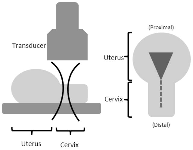
A schematic diagram of the experimental set up is shown in Fig. 1. The transducer was aligned parallel to the endocervical canal and SWS data were acquired from each specimen at 3 cm depth (close to elevational focus) with a saline acoustic path for acoustic coupling. A 5×5 mm region of interest (ROI) for SWS measurement was placed about midway through the thickness (about 7mm deep – the thickness for each half was 13.6±0.19 mm; mean±1 SD) of the cervical canal and measurements were made at 4–5 non-overlapping locations along the length of the cervix. Five repeat measurements were made at each location to improve estimate precision.
Fig. 1.
A schematic diagram of the experimental setup. (Right) View of half a cervix from above. The dashed line indicates the endocervical canal and triangle is uterine cavity. (Left) View from the side of a cervix half. The transducer is aligned parallel to endocervical canal and focused mid-depth through the cervix indicated by lateral beam contours.
All data processing was performed offline with MATLAB (The MathWorks). Tissue motion from the acoustic radiation force was measured by the Loupas Method on I-Q echo data19. A threshold of 0.98 was used for complex correlation coefficient magnitude between consecutive frames of data to remove poor displacement estimates. A low pass filter with a cutoff at 1 kHz was used to remove high frequency jitter in displacement estimates. The shear wave speed was estimated in the remaining data using the RANSAC algorithm described by Wang et al.20.
C. Data Analysis
The mean cervical length was 2.79±0.38 cm. To standardize measurement locations among cervices of different lengths, the cervical canals were partitioned based on fractional distances from the internal os. The distal and proximal ends (external and internal os, respectively) were identified by a Maternal-Fetal Medicine subspecialist (HF) on the B-mode images, as illustrated in Fig. 2, and measurements were made between these endpoints. Regions that included cystic structures were avoided because such structures would perturb shear wave propagation. Each SWS estimation location was labeled based on fractional length (FL) from the proximal end as follows: 0.05–0.25 - proximal, 0.26–0.44 - mid-proximal, 0.45–0.55 - mid, 0.56–0.75 - mid-distal, and 0.76–0.95 - distal. In some cases, only four measurements were made on cervices that were shorter. To get a mid measurement, a value was interpolated from the mid-proximal and mid-distal locations.
Fig. 2.
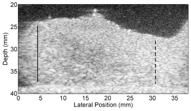
B-mode image of half of a bivalved cervix sample. The endocervical canal is located at the top, the distal end is on the left and proximal end/uterus is on the right. The bright line on the bottom is the SoAb rubber interface. The solid lines mark the distal end (external os) and the dashed lines the proximal end (internal os). These locations were verified by HF (the Maternal Fetal Medicine subspecialist co-author). Measurements were made between these endpoints.
D. Statistical Analysis
Statistical analysis was performed to (1) evaluate SWS variability as a function of location along the length of the canal; (2) evaluate SWS as a function of anterior/posterior cross sectional position; and (3) evaluate SWS as a function of ripening. A linear mixed model was used to represent SWS as a function of anterior vs. posterior plane, location (fixed effects/independent of a particular cervix), ripened vs. unripened, and individual cervix (random effects/dependent on a particular cervix). Location was converted to a numerical variable based on fraction length (FL) from the external os (0 = distal, 0.25 = mid-distal,...1 = proximal) and all other variables were treated as binary (0 or 1) as summarized in Table II. A sequential model building strategy was used to test each hypothesis based on a likelihood ratio F-test to assess the improvement in the fit between the model and the SWS estimates at each step in the model with a p<0.05 (two-sided) criterion for significance. Maximum Likelihood values were selected in model construction. Diagnostic and exploratory plots were used to assess any possible violations in model assumptions. Statistical analyses were performed in R (R Foundation, Vienna, Austria) with the ‘nmle’ package21;22. The models were as follows:
TABLE II.
Summary of Linear Mixed Model Variables. Location refers to the length along the canal (fractional length (FL)).
| Variable | Name | Numerical Type | Values |
|---|---|---|---|
| Location | FL | Integer | Distal = 0 Mid-Distal = 0.25 Mid = 0.5 Mid-Proximal = 0.75 Proximal = 1 |
| Anterior/Posterior | AP | Binary | Anterior = 0 Posterior = 1 |
| Ripened/Unripened | Ripe | Binary | Ripened = 0 Unripened = 1 |
1) Model 1: Basic Additive Model
This was the base model consisting of all terms listed in Table II using only fixed effects for all variables. This model results in a single slope (b′) in SWS as a function of fractional length (FL) along the canal for all specimens but the intercepts can vary for each specimen. This model can be interpreted as:
| (2a) |
| (2b) |
Lower case letters (with/without apostrophe) denote fixed or random effect coefficients for each variable, respectively.
2) Model 2: Model 1 + Location/(Anterior vs. Posterior) Interaction
The term FL * AP was introduced into Model 1 to allow for differences in the gradient in SWS along the canal between anterior and posterior slices.
| (3a) |
| (3b) |
3) Model 3: Model 2 + (Anterior vs. Posterior)/Ripe Interaction Term
The term AP * Ripe was introduced to Model 2 allow for differences between ripened vs. unripened and anterior vs. posterior. This model allows for differences in SWS slope between groups of specimens (anterior v. posterior slices; ripened v. unripened specimens), but requires, for example, that the slope of the SWS for all unripened specimens in the anterior plane to be the same.
| (4a) |
| (4b) |
4) Model 4: Modified Model 3 with Randomized Slope Term
Model 3 was modified to allow for differences in SWS along the canal for different groups of specimens. Model 4 allows for variability in SWS slope along the canal among individuals (i), but it retains the fixed effect of anterior vs. posterior slice orientation.
| (5a) |
| (5b) |
5) Model 5: Modified Model 4 with Randomized Anterior vs. Posterior Intercept Term
Model 4 was modified to allow for variability in SWS slope along the canal among individuals including individual variability for the effect of anterior v. posterior slice orientation.
| (6a) |
| (6b) |
6) Model 6: Model 5 + Location/Ripe Interaction Term
The term FL * Ripe was introduced into Model 5 to allow for differences in slope between ripened and unripened. This was the final model for the mean SWS for each group, with fixed effects (random effects bi average to zero for all samples) coefficients shown in equation 9 below.
| (7a) |
| (7b) |
7) Model 7: Model 6 + Location/Ripe/(Anterior vs. Posterior) Interaction Term
The term FL * Ripe * AP was introduced into Model 6 to allow for differences in slope between ripened and unripened as well as anterior vs. posterior. The addition of this variable resulted in a p-value of 0.78 (a non-significant improvement over Model 6).
| (8a) |
| (8b) |
It is important to note that the ripened group (n=13) contained both subjects who received a prostaglandin agent (n=7) and subjects who were experiencing uterine bleeding at the time of surgery (n=6). Endogenous prostaglandins are known to be associated with cramping and cervical softening 23–26. An exogenous prostaglandin (misoprostil) is used clinically to soften the cervix for many obstetric and gynecology exams27–30. Data are not shown here, but linear mixed model found no significant difference between misoprostil ripened and uterine bleeding/cramping groups (p = 0.86). This justified combining groups to increase statistical power.
To test the ability of SWS estimates to correctly classify ripened versus unripened cervix tissue, receiver operating characteristic (ROC) curves and area under the curve (AUC) were calculated for the mid location in anterior vs. posterior data. If a mid location did not exist for a particular sample (only 4 locations measured instead of 5) then a “mid” location was interpolated by averaging the mid-distal and mid-proximal estimates.
III. Results
A. Linear Mixed Model
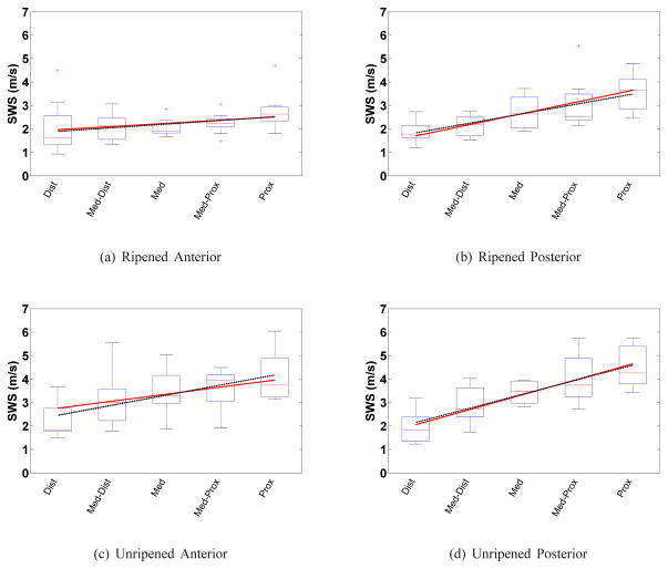
Shear wave speed increased from the distal to proximal end for all samples. Fig. 3 shows the box plot of the mean SWS for anterior/posterior slices for the ripened and unripened groups. The linear mixed model for each group and location as defined by equation (9):
| (9) |
Fig. 3.
Box plots of the mean SWS from each sample vs. cervical canal location for each group and cervix half for: ripened (a–b), and unripened (c–d); anterior (left column) and posterior (right column) slices. The boxes represent the interquartile range (IQR) among SWS estimates, the horizontal line near the middle of each box is the median value for that group, the whiskers represent the maxima and minima within 1.5*IQR, and crosses are outliers outside of 1.5*IQR. The solid line spanning the boxes is the mixed model fit based on equation 9. Similarly, the dashed line is the linear regression result for the mean SWS in that group. The linear regression does not take into account the repeated measures within the same specimen, whereas the mixed model does.
This form is shorthand for the four fits in Fig. 3 corresponding to the four combinations of the binary variables AP and Ripe. The coefficients are fixed effects coefficients representing an average over all samples. The random effects were necessary to seperate average vs. individual components to capture variation between subjects. The corresponding likelihood ratio F-test results of adding each variable are shown in Table III to justify the addition of each variable in Model 6. Most variables were found to be significant (p<0.05) with the exception of FL * Ripe but the p-value was only slightly over 0.05 (p = 0.0534) possibly due to limited sample size and was included after sequentially building upon each model. Therefore Model 6 was chosen as the best fit to the data set.
TABLE III.
Likelihood ratio F-Test results of Sequential Model Building
| Test | Added Term | Likelihood Ratio | P-value |
|---|---|---|---|
| 1 vs. 2 | FL * AP | 50.02 | < 0.0001 |
| 2 vs. 3 | Ripe * AP | 5.58 | 0.02 |
| 3 vs. 4 | Random FL | 243.63 | < 0.0001 |
| 4 vs. 5 | Random FL * AP | 517.48 | < 0.0001 |
| 5 vs. 6 | Ripe * FL | 3.73 | 0.0534 |
| 6 vs. 7 | AP * Ripe * FL | 0.08 | 0.78 |
A comparison among mixed and linear regression model SWS slopes is shown in Table IV. The unripened group showed the greatest increase in SWS from distal to proximal end. The ripened group showed a smaller increase in SWS from distal to proximal end for both anterior and posterior. That group also had lower variance in SWS among specimens than the unripened group. The linear least squares fit was computed to individually assess the SWS vs. location gradient (dashed line). The slopes for posterior data, compared to anterior, were larger for both ripened and unripened specimens. As expected, the linear mixed model slopes for each group are very similar to the respective linear regression results.
TABLE IV.
Shear wave speed gradient (m·s−1· FL−1) along the cervical canal determined by the linear mixed effects model (equation 9) and linear regression for individual groups.
| Linear Mixed Effects | Linear Regression | |
|---|---|---|
| Ripened Anterior | 0.54 | 0.62 |
| Ripened Posterior | 1.94 | 1.66 |
| Unripened Anterior | 1.2 | 1.72 |
| Unripened Posterior | 2.60 | 2.44 |
B. Classification of Ripened vs. Unripened
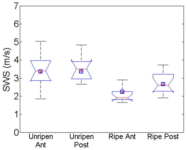
To make future comparisons between unripened and ripened in a clinical setting, a standardized location along the length of the canal needed to be chosen. The largest difference between ripened and unripened occurred at the proximal location and the least difference at the distal location. Due to feasibility concerns in a clinical setting (e.g., proximity to the fetal membranes and fetal head), the mid location was chosen 18. Fig. 4 shows a box plot of mean SWS at the mid location for anterior and posterior slices for both ripened and unripened groups. The notches in the box plot indicate the 95% confidence interval for the median for that group. The black diamonds indicate predicted values with the linear mixed model and the blue squares are values from the least squares regression model. The unripened anterior and posterior data are likely equivalent to each other. The ripened anterior and posterior data are roughly equivalent to each other, but both are outside the 95% confidence interval for the unripened data. The mean SWS estimate values from the samples for unripened were 3.45±0.97 m/s, 3.56±0.92 m/s for anterior and posterior, respectively. The ripened group SWS estimates were significantly less, 2.11±0.45 m/s, 2.68±0.57 m/s (p< 0.001). In Fig. 4, the predicted SWS estimates for both linear regression and mixed model at the mid-location are near the respective median value and well within the interquartile range.
Fig. 4.
Boxplot of mean SWS at mid location for each group; Unripened Anterior, Unripened Posterior, Ripened Anterior, and Ripened Posterior respectively. The notches indicate 5% significance if two intervals do not overlap. The diamonds indicate the SWS predicted using the linear mixed model and squares are least squares predicted value.
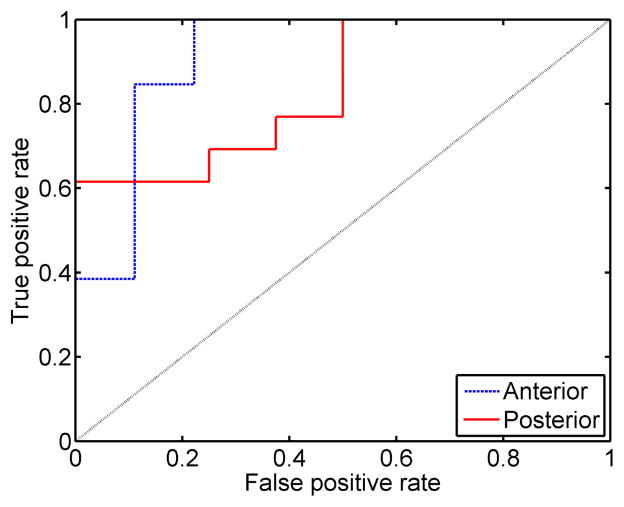
To test the ability to discriminate ripened from unripened cervix tissue based on estimates of SWS at the mid location, the ROC curve was calculated and is shown in Fig. 5. A positive condition was a ripened cervix sample. The ROC curve for anterior data is shown as a dashed line and posterior a solid line. The dotted black line shows a 50% chance of correctly identifying a ripened cervix. The AUC values were 0.91 (anterior) and 0.84 (posterior). The sensitivity for anterior and posterior mid location SWS estimates were 85% and 69%. The corresponding specificity values were 89% and 75% for anterior and posterior, respectively at the operating point of maximum combined sensitivity and specificity. The corresponding SWS thresholds were 2.37 m/s and 3.02 m/s for anterior and posterior, respectively. Power was not computed a priori, but with n = 22, a two sample Student’s t-test can detect a difference of 0.86 standard deviations with 80% power at the 5% significance level.
Fig. 5.
Empirical receiver operating characteristic curves (ROC) for anterior (dashed) and posterior (solid) SWS mean SWS estimates at the mid location with a positive assigned to ripened tissue.
C. SWS vs. Thickness
A test was performed to investigate the potential for Lamb wave propagation, as opposed to shear wave propagation, due to large wavelength of the observed transverse waves compared to the thickness of the cervix wall. (Lamb wave speed for a given material is proportional to the ratio of the material thickness and the wavelength of the disturbance31;32). The estimated transverse wave speeds among unripened tissue specimens were compared to the cervical wall thickness for each specimen, and linear regression was used to determine if there was any correlation between these variables. Fig. 6 shows mean transverse wave speeds at the mid location vs. cervical thickness from each half for anterior (asterisks) and posterior (circles). The corresponding least squares coefficient of determination (r2) values were 0.22 and 0.002 for anterior and posterior, respectively. This suggests there is no correlation between cervix wall thickness and the estimated transverse wave speed.
Fig. 6.
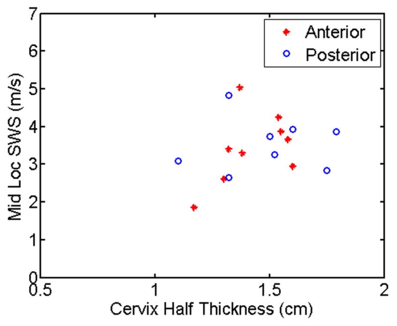
Mean SWS from the mid location for each unripened cervix half vs. thickness (radius of cervix).
IV. Discussion
The goal of this study was to characterize the spatial and biological variability among SWS estimates in the cervix using a multivariate analysis and to assess the suitability of SWS for predicting ripened vs. unripened state. Due to the complexity of cervical microstructure, this is necessary for a comprehensive understanding of tissue properties for future development of an objective method for monitoring the cervix during pregnancy.
Pertaining to spatial variability, we found that there is consistent spatial variability along the length of the cervix as well as a difference in anterior vs. posterior slices among samples, as shown in Fig. 3. Interestingly, this gradient in SWS values is larger on the posterior half of the cervix for both ripened and unripened groups, which explains the need for including the FL * AP interaction into model 6. The linear mixed model shows that the variables for position along the canal (fractional length; FL) and cervix half (AP) both influence SWS estimates with p-values < 0.05 confirming our observations. The model also shows a clear difference between ripened and unripened tissue indicated by the variable accounting for ripening (Ripe) which shifts the intercept up and down. In particular, the model found correlation between slope anterior vs. posterior and slope and ripening (although p-value was 0.0534). This suggests as the cervix ripens, it become more uniform spatially. Overall, the linear mixed model shows a relatively good fit to experimental data and only small deviations from the least squares fit which strengthens the validity of our model.
Due to the significance of location on SWS estimates, we chose a consistent measurement location to make comparisons between ripened and unripened groups. Fig. 4 shows there is a significant difference between ripened and unripened samples for both anterior and posterior slices (no overlap in the 95% confidence interval comparing ripened to unripened specimens) at the mid location. The linear mixed model and least square predictions are also within the respective IQR indicating a good fit. Fig. 5 shows the corresponding empirical ROC curves calculated from these SWS estimates. The AUC of 0.91 for the anterior slices suggests promise for discriminating ripened from unripened cervix tissue. However, the lower AUC for the posterior slices, while still demonstrating good performance, illustrates that these ROC curves are undersampled and no strong statements can be made until more data are available.
Due to the small size of the cervix relative to the shear wave length (thickness of each half was 13.6±0.19 mm) compared to the wavelength of the induced transverse wave (22±6 mm for unripened anterior mid location), there was concern regarding the potential for Lamb wave behavior (wave speed proportional to the ratio of the cervix wall thickness and the wavelength of the disturbance). Results in Fig. 6 show no correlation between SWS and cervix radius suggesting the appropriate model for wave propagation is not a simple low order Lamb wave in isotropic media. But, the wave also cannot strictly be considered a shear wave due to the boundary conditions. The most appropriate label for these waves is likely a “pseudo-transverse” or “pseudo-shear” wave32. However, to avoid confusion in the medical elastography literature, and to be consistent with prior use of the term “shear waves” under similar conditions in the technical literature [see, for example, Gennisson et al.33], we chose to continue to use the term “shear waves” to refer to the general class of transverse waves created with acoustic radiation force.
The model clearly supports the observation that there is an increase in SWS along the length of the canal and that the slope among posterior slices is higher than anterior. It was suggested in our earlier work that the anterior mid position would be the preferred location 18. Based upon our ROC analysis, this is a reasonable suggestion. We claim that the ripened group will more closely resemble the pregnant cervix. The lower variance and slope in the ripened group suggests that, as pregnancy progresses, the significance of small deviations in positioning will become less important since the cervix likely becomes less heterogeneous as found using invasive techniques in animal models34;35.
One limitation of our study was the assumption that SWS is constant throughout a 5×5mm ROI. Fig. 3 demonstrates SWS changes at discrete locations along the canal, but it is more likely that the SWS continuously increases from the distal to proximal end. This would suggest the shear wave accelerates as it propagates along the canal and the time-to-peak data would be better modeled with a quadratic function instead of a linear fit20. Fig. 7 shows a time-to-peak estimate from one measurement and location of an unripened sample averaged over a full (5 mm) axial range vs. lateral location for one SWS estimate. The dashed line shows the typical linear fit (constant SWS) for time to peak data and the dotted line shows a quadratic fit (constant acceleration in SWS of 0.99 m·s−1·cm−1). This figures shows that due to noise in displacement estimates, a small increase in SWS (<1 m·s−1·cm−1) over a 5mm lateral span is not resolvable with these methods. This suggests that acceleration of the shear wave within the ROI has minimal affect on the SWS estimate. Also, these slopes in SWS estimates along the canal suggest that if measurement location varies within a few millimeters, the SWS estimates will not change significantly.
Fig. 7.
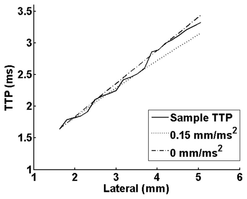
Time-to-peak (TTP in ms) vs. lateral location for one SWS measurement. The sample TTP is shown as a solid line and was averaged over the full 5mm axial range. A simulated TTP for a constant SWS estimate of 1.91 m/s (dashed) and a simulated TTP for a constant increase in SWS of 0.99 m·s−1cm−1 (dotted).
Another limitation of our study is the use of a probe unsuitable for in vivo study. This transducer had a much larger aperture (38 mm) that could cover the entire length of the cervix to reduce measurement time. A smaller aperture array, such as the 14 mm prototype endocavity transducer 36, would be more applicable to in vivo use. Such an array is small enough to fit inside the vagina and be placed along the cervical canal. It is also capable of producing high intensity, long duration ultrasound pulses necessary for shear wave imaging. We have performed initial testing and simulations to compare performance of the larger commercial array and the prototype array and found similar performance. However, for this study, the prototype array was impractical to acquire the large data set needed to investigate spatial variability in SWS estimates.
Each sample was bivalved in order to measure from the inside surface the canal (we initially thought placing the prototype transducer inside the cervical canal had advantages). The cervix contains a large circumferential band of collagen, and severing this layer likely relieves stress/tensile strain and changes mechanical properties. It should also be mentioned that loading conditions in vivo will likely be different. In our initial studies in pregnant women involve placement of a clinician’s finger on the cervix which may add variance to repeat measurements (due to initial preload). In addition, samples were brought from body temperature to room temperature which likely effects mechanical properties. Furthermore, one significant assumption was that there was no dispersion present. The shear waves in the unripened anterior mid location had a center frequency of about 100Hz and a −6 dB bandwidth of 200Hz. Using shear waves with different spectral content may have significant implications on the viscoelastic behavior of cervical tissue, resulting in biased group velocities36. While the SWS estimates found in this paper may not be representative of the true in vivo SWS values, the experiments were well controlled and trends found should remain consistent.
V. Conclusions
In summary, shear wave speed estimation should provide an excellent tool for eventual calculation of an elastic modulus, and a more targeted approach to evaluating the cervix. Due to the large spatial variability (1.2 m·s−1·FL−1 for anterior) within the unripened cervix, knowing the specific location along the canal becomes increasingly important. However, during pregnancy the cervix will likely be more similar to the ripened cervix (0.54 m·s−1·FL−1 for anterior) and small changes in location will likely have little impact on measurements. Our study has shown that if the location is accounted for, comparisons between patients and can distinguish between ripened vs. unripened subjects. The transition into in vivo study should not be difficult and preliminary results are encouraging.
Acknowledgments
This work was supported by NIH Grants T32CA009206, R21HD061896, R21HD063031 and R01HD072077 from the Eunice Kennedy Shriver National Institute of Child Health and Human Development. The authors would also like to recognize Dr. Michael Wang for providing RANSAC code, Dr. Paul Urie and Deanna Staker, PA-C in the Pathology Department at Utah Valley Regional Medical Center for their invaluable assistance. We are grateful to Siemens Medical Solutions for the equipment loan and technical support that made this study possible.
References
- 1.Read CP, Word RA, Ruscheinsky MA, Timmons BC, Mahendroo MS. Cervical remodeling during pregnancy and parturition: molecular characterization of the softening phase in mice. Reproduction. 2007 Aug;134(2):327–340. doi: 10.1530/REP-07-0032. [DOI] [PubMed] [Google Scholar]
- 2.Word RA, Li XH, Hnat M, Carrick K. Dynamics of cervical remodeling during pregnancy and parturition: Mechanisms and current concepts. Semin Reprod Med. 2007 Jan;25(1):69–79. doi: 10.1055/s-2006-956777. [DOI] [PubMed] [Google Scholar]
- 3.Akins ML, Luby-Phelps K, Mahendroo M. Second harmonic generation imaging as a potential tool for staging pregnancy and predicting preterm birth. J Biomed Opt. 2010 May;15(2):026020. doi: 10.1117/1.3381184. [DOI] [PMC free article] [PubMed] [Google Scholar]
- 4.Hassan SS, Romero R, Vikyadhari D, Fusey S, Baxter J, Khandelwal M, Vijayaraghavan J, Trivedi Y, Soma-Pillay P, Sambarey P, Dayal A, Potapov V, O’Brien J, Astakhov V, Yuzko O, Kinzler W, Phillips JA, Creasy GW and for the PREGNANT Trial, . Vaginal progesterone reduces the rate of preterm birth in women with a sonographic short cervix: a multicenter, randomized, double-blind, placebo-controlled trial. Ultrasound Obstet Gynecol. 2011 Jul;38(1):18–31. doi: 10.1002/uog.9017. [DOI] [PMC free article] [PubMed] [Google Scholar]
- 5.Parra-Saavedra M, Gmez L, Barrero A, Parra G, Vergara F, Navarro E. Prediction of preterm birth using the cervical consistency index. Ultrasound Obstet Gynecol. 2011 Jul;38(1):44–51. doi: 10.1002/uog.9010. [DOI] [PubMed] [Google Scholar]
- 6.Dubrauszky V, Schwalm H, Fleischer M. Fibre system of connective tissue in childbearing age, menopause, and pregnancy. Arch Gynakol. 1971;210(3):276. doi: 10.1007/BF00667740. [DOI] [PubMed] [Google Scholar]
- 7.Hukins DWL, Aspden RM. Composition and properties of connective tissues. Trends Biochem Sci. 1985 Jul;10(7):260–264. [Google Scholar]
- 8.Aspden RM. Collagen organization in the cervix and its relation to mechanical function. Coll Relat Res. 1988;8(2):103–112. doi: 10.1016/s0174-173x(88)80022-0. [DOI] [PubMed] [Google Scholar]
- 9.Breeveld-Dwarkasing VN, de Boer-Brouwer M, Tekoppele JM, Bank RA, van der Weijden C, Taverne MA, van Dissel-Emiliani FMF. Regional differences in water content, collagen content, and collagen degradation in the cervix of nonpregnant cows. Biol Reprod. 2003;69(5):1600–1607. doi: 10.1095/biolreprod.102.012443. [DOI] [PubMed] [Google Scholar]
- 10.Breeveld-Dwarkasing VN, Tekopele JM, Bank RA, van der Weifden C, Taverne MA, van Dissel-Emiliani FMF. Changes in water content, collagen degradation, collagen content and concentration on repeat biopsies of the cervix of pregnant cows. Biol Reprod. 2003;69(5):1608–1614. doi: 10.1095/biolreprod.102.012534. [DOI] [PubMed] [Google Scholar]
- 11.Feltovich H, Hall TJ, Berghella V. Beyond cervical length: emerging technologies for assessing the pregnant cervix. Am J Obstet Gynecol. 2012 Nov;207(5):345–354. doi: 10.1016/j.ajog.2012.05.015. [DOI] [PMC free article] [PubMed] [Google Scholar]
- 12.Swiatkowska-Freund M, Preis K. Elastography of the uterine cervix: implications for success of induction of labor. Ultrasound Obstet Gynecol. 2011 Jul;38(1):52–56. doi: 10.1002/uog.9021. [DOI] [PubMed] [Google Scholar]
- 13.Molina FS, Gómez LF, Florido J, Padilla MC, Nicolaides KH. Quantification of cervical elastography: a reproducibility study. Ultrasound Obstet Gynecol. 2012 Jun;39(6):685–689. doi: 10.1002/uog.11067. [DOI] [PubMed] [Google Scholar]
- 14.Hernandez-Andrade E, Hassan SS, Ahn H, Korzeniewski SJ, Yeo L, Romero R. Evaluation of cervical stiffness during pregnancy using semiquantitative ultrasound elastography. Ultrasound Obstet Gynecol. 2013 Feb;41(2):152–161. doi: 10.1002/uog.12344. [DOI] [PMC free article] [PubMed] [Google Scholar]
- 15.Torr GR. The acoustic radiation force. Am J Phys. 1984;52(5) [Google Scholar]
- 16.Sarvazyan AP, Rudenko OV, Swanson SD, Fowlkes J, Emelianov SY. Shear wave elasticity imaging: a new ultrasonic technology of medical diagnostics. Ultrasound Med Biol. 1998;24(9):1419–1435. doi: 10.1016/s0301-5629(98)00110-0. [DOI] [PubMed] [Google Scholar]
- 17.Lai WM, Rubin DH, Rubin D, Krempl E. Introduction to continuum mechanics. Burlington, MA: Butterworth-Heinemann; 2009. [Google Scholar]
- 18.Carlson LC, Feltovich H, Palmeri ML, Dahl JJ, del Rio A, Hall TJ. Shear wave speed estimation in the human uterine cervix. Ultrasound Obstet Gynecol. 2013 doi: 10.1002/uog.12555. [Online]. Available: http://dx.doi.org/10.1002/uog.12555. [DOI] [PMC free article] [PubMed]
- 19.Pinton G, Dahl J, Trahey G. Rapid tracking of small displacements with ultrasound. IEEE Trans Ultrason, Ferroelectr, Freq Control. 2006 Jun;53(6):1103–1117. doi: 10.1109/tuffc.2006.1642509. [DOI] [PubMed] [Google Scholar]
- 20.Wang MH, Palmeri ML, Rotemberg VM, Rouze NC, Nightingale KR. Improving the robustness of time-of-flight based shear wave speed reconstruction methods using ransac in human liver in vivo. Ultrasound Med Biol. 2010 May;36(5):802–813. doi: 10.1016/j.ultrasmedbio.2010.02.007. [DOI] [PMC free article] [PubMed] [Google Scholar]
- 21.R Development Core Team. R: A Language and Environment for Statistical Computing. R Foundation for Statistical Computing; Vienna, Austria: 2011. [Online]. Available: http://www.R-project.org/ [Google Scholar]
- 22.Pinheiro JC, BDM . Mixed-effect models in S and S-Plus. New York: Springer; 2000. [Google Scholar]
- 23.Clark K, Myatt L. Prostaglandins and the reproductive cycle. CD-ROM: Gynecology and Obstetrics. 2004;5 [Google Scholar]
- 24.Pulkkinen MR, Henzl MO, Csapo AI. The effect of naproxen-sodium on the prostaglandin concentrations of the menstrual blood and uterine “jet-washing” in dysmenorrehic women. Prostaglandins. 1978 Mar;13(1):543–550. doi: 10.1016/0090-6980(78)90138-7. [DOI] [PubMed] [Google Scholar]
- 25.Chan WY, Dawood MY. Prostaglandin levels in menstrual fluid of nondysmenorrheic and dysmen-orrheic subjects with and without oral contraceptive on ibuprofen therapy. Adv Prostaglandin Thromboxane Res. 1980;8:1443–1447. [PubMed] [Google Scholar]
- 26.Pickles V, Hall W, Best F, Smith G. Prostaglandins in endometrium and menstrual fluid from normal and dysmenorrhoiec subjects. J Obstet Gynaecol Br Commonw. 1965 Apr;72:185–192. doi: 10.1111/j.1471-0528.1965.tb01415.x. [DOI] [PubMed] [Google Scholar]
- 27.Allen R, O’Brien BM. Uses of misoprostol in obstetrics and gynecology. Rev Obstet Gynecol. 2009;2(3):159–168. [PMC free article] [PubMed] [Google Scholar]
- 28.Crane JM, Healey S. Use of misoprostol before hysteroscopy: a systematic review. J Obstet Gynaecol Can. 2006;28(5):373–379. doi: 10.1016/s1701-2163(16)32150-8. [DOI] [PubMed] [Google Scholar]
- 29.Kelly AJ, Malik S, Smith L, Kavanagh J, Thomas J. Vaginal prostaglandin (pge2 and pgf2a) for induction of labour at term. Cochrane Database Syst Rev. 2009 Oct;7(4):CD003101. doi: 10.1002/14651858.CD003101.pub2. [DOI] [PubMed] [Google Scholar]
- 30.Hofmeyr GJ, Gulmezoglu AM, Pileggi C. Vaginal misoprostol for cervical ripening and induction of labour. Cochrane Database Syst Rev. 2010 Oct;6(10):CD000941. doi: 10.1002/14651858.CD000941.pub2. [DOI] [PMC free article] [PubMed] [Google Scholar]
- 31.Viktorov IA. Rayleigh and Lamb waves: physical theory and applications. Vol. 147 Plenum press; New York: 1967. [Google Scholar]
- 32.Auld B. Acoustic Fields and Waves in Solids. 1&2 Malabar, FL: Krieger; 1973. [Google Scholar]
- 33.Gennisson JL, Grenier N, Combe C, Tanter M. Supersonic shear wave elastography of invivo pig kidney: Influence of blood pressure, urinary pressure and tissue anisotropy. Ultrasound Med Biol. 2012;38(9):1559–1567. doi: 10.1016/j.ultrasmedbio.2012.04.013. [DOI] [PubMed] [Google Scholar]
- 34.Myers K, Socrate S, Tzeranis D, House M. Changes in the biochemical constituents and morphologic appearance of the human cervical stroma during pregnancy. Eur J Obstet Gynecol. 2009 May;144(S1):S82–S89. doi: 10.1016/j.ejogrb.2009.02.008. [DOI] [PubMed] [Google Scholar]
- 35.Zhang Y, Akins ML, Murari K, Xi J, Li MJ, Luby-Phelps K, Mahendroo M, Li X. A compact fiber-optic shg scanning endomicroscope and its application to visualize cervical remodeling during pregnancy. Proc Natl Acad Sci U S A. 2012 Aug;109(32):12 878–12 883. doi: 10.1073/pnas.1121495109. [DOI] [PMC free article] [PubMed] [Google Scholar]
- 36.Palmeri ML, Feltovich H, Homyk AD, Carlson LC, Hall TJ. Evaluating the feasibility of acoustic radiation force impulse shear wave elasticity imaging of the uterine cervix with an intracavity array: a simulation study. IEEE Trans Ultrason, Ferroelectr, Freq Control. 2013 Oct;60(10):2053–2064. doi: 10.1109/TUFFC.2013.2796. [DOI] [PMC free article] [PubMed] [Google Scholar]


