Abstract
Considering the high morbidity of hepatitis B in China, many epidemiological studies based on classic medical statistical analysis have been started but lack spatial information. However, spatial information such as the spatial distribution, autocorrelation and risk factors of the disease is of great help in studying patients with hepatitis B. This study examined 2851 cases of hepatitis B that were hospitalized in Shenzhen in 2010 and studied the spatial distribution, risk factors and spatial access to health services using spatial interpolation, Pearson correlation analysis and the improved two-step floating catchment area method. The results showed that the spatial distribution of hepatitis B, along with risk factors as well as spatial access to the regional medical resources, was uneven and mainly concentrated in the south and southwest of Shenzhen in 2010. In addition, the distribution characteristics of hepatitis B revealed a positive correlation between four types of service establishments and risk factors for the disease. The Pearson correlation coefficients are 0.566, 0.515, 0.626, 0.538 corresponding to bath centres, beauty salons, massage parlours and pedicure parlours (p < 0.05). Additionally, the allocation of medical resources for hepatitis B is adequate, as most patients could be treated at nearby hospitals.
Keywords: spatial epidemiology, spatial analysis, hepatitis B, Shenzhen
1. Introduction
The hepatitis B virus (HBV) is one of the most common viral infections in the world, leading to many deaths each year from associated liver diseases [1,2]. HBV is also an important public health issue in China [2], as national surveys conducted since the 1970s have repeatedly showed high morbidity from HBV infections in the general population [3,4]. To address this challenge, many scholars now to study the disease using different approaches (e.g., pathology, immunology and epidemiology), but none of these approaches incorporate spatial information [5]. With the development of Geographic Information System (GIS) technology and its applications in epidemiology [6], it has become clear the spatial information has great value in Epidemiology. Spatial epidemiology is a branch of epidemiology that uses spatial information to extend the analysis of disease distribution and risk factors. This information serves as a powerful analytical tool for epidemiological studies and will likely show greater significance in the future [7]. Our team have done some works on spatial epidemiology [8,9,10].
Using geographic information systems and spatial analysis technology, spatial epidemiology attempts to describe and analyze human diseases, including the spatial distribution characteristics of health and hygiene events as well as the regularity of changes and developments. Spatial epidemiology also explores the decisive elements that can impact public health and provides strategies and measures for disease prevention and cure and health promotion and hygiene services [7,11]. Research on this subject mainly utilizes four elements: disease mapping, risk assessment in relation to a point or line source, disease clustering analysis and geographical correlation studies [11]. Disease mapping is the most important tool in spatial epidemiology and is used to describe and evaluate disease area distribution [7]. The most typical example of disease mapping is the epidemiological investigation of a cholera outbreak caused by street water pollution in London in 1854 [12,13]. The assessment of risk factors is similar to geographical correlation studies in that they both focus on studying cause of geographical phenomenon. Moreover, analysis of disease clustering uses statistical methods to identify disease spatial aggregation, thus providing corresponding methods to search for etiologic clues [7,14,15].
Among the four study elements, disease mapping and disease clustering analysis are relatively mature, and typical methods and models, such as spatial interpolation and spatial scan statistics are commonly used [16,17,18]. However, exploring the risk factors for disease is complex and difficult, especially for diseases in which it is difficult to obtain patient exposure information, and data involving patients’ privacy [7]; this challenge represents a weak link in epidemiological studies. Compared with other infectious diseases such as schistosomiasis [19,20], most respiratory system diseases [21] and cardiovascular diseases [8], the spatial risk factors for hepatitis B are less obvious, and there have been few studies on this aspect. In view of this problem, this study sought to explore the spatial risk factors for hepatitis B and to discover the relationship between these risk factors and hepatitis B morbidity.
In addition, the prevention and control of disease is the main goal of spatial epidemiology, and one important research subject is spatial access to health services. Spatial access to health services refers to overcoming spatial obstacles to medical facilities [22,23]. Based on different application environments and requirements, many different research methods are used to measure spatial access. Among the numerous methods, the gravity model (also known as the potential model) and the two-step floating catchment area method are the most widely used [24,25]. However, both methods have flaws; the gravity model is somewhat abstract and difficult to understand, and the two-step floating catchment area method ignores the spatial access differences in demand points within the same search scope and the spatial access values in demand points outside of the search scope [26]. It is also difficult to set a reasonable search radius for each medical facility [27]. This current study used an improved two-step floating catchment area model to overcome these limitations. In particular this model considers the effect of distance decay by setting weighted distance values, and this improved method is also an effective method for setting a reasonable search radius for each medical facility. These two changes significantly improve the accuracy of measuring spatial access to health services.
2. Data and Methods
2.1. Study Area
Shenzhen is a coastal city located in the south of China, northeast of the Pearl River Estuary. This city is located south of the Tropic of Cancer, from 113°46′ to 114°37′ east longitude and between 22°27′ and 22°52′ north latitude, and the total area of Shenzhen is approximately 1952.84 km2 [27].
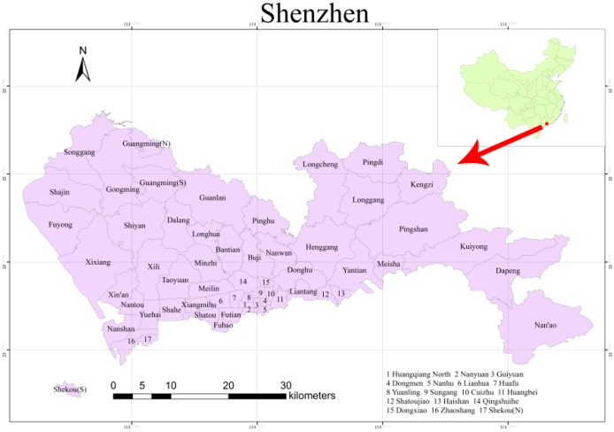
Shenzhen is located at the border between subtropical monsoon and tropical marine climates with abundant rainfall and beautiful scenery. The average annual precipitation is approximately 1924.7 mm. With 230 km of coastline, Shenzhen is rich in marine resources such as excellent ports and abundant fisheries. Shenzhen was the first special economic zone in China. With its rapid economic development, Shenzhen occupies a position of importance in China. At present, there are a total of 10 districts and 57 sub-districts in Shenzhen. Figure 1 shows the location of Shenzhen in China and the names of its sub-districts.
Figure 1.
The study area.
2.2. Study Data
The study area for this paper was the whole of Shenzhen City, which includes 10 districts and 57 sub-districts. The study mainly collected geographic, demographic, and hepatitis B case data, along with some service facility and medical resource data:
Basic geographic data: Administrative data for the division of Shenzhen were obtained from the Urban Planning, Land and Resources Commission of the Shenzhen Municipality [9].
Demographic data: These data, for all 57 different sub-district administrative regions, were obtained from the 6th national population census [28].
Hepatitis B case data: Data from the Shenzhen Centre for Health Information (SCHI), an institute directly administered by the Health, Population and Family Planning Commission of Shenzhen Municipality, were obtained from hospitalized patients’ medical records including the patients’ home addresses, ages, sexes, etc. in 2010.
Medical facility data: These data were also obtained from the Shenzhen Centre for Health Information with addresses and service levels for most hospitals.
Service facility data: Certain service facilities may promote hepatitis B infection. Address data were obtained by searching electronic maps on the Internet.
2.3. Study Methods
This study mainly applied spatial interpolation (Kriging), spatial risk factors correlation analysis and analysis of spatial access to health services. To be pointed out that the Shenzhen Center for Health Information (SCHI), an institute directly administered by the Health, Population and Family Planning Commission of Shenzhen Municipality gave the permission of the research involving hepatitis B cases and approved this retrospective study. In this study, written informed consent was obtained by participants so we could not reveal their personal information to the public. In addition, the study was approved by the Wuhan University Institutional Ethnic Committee, and we must keep the patients’ information secret.
2.3.1. Spatial Interpolation
Spatial interpolation is a process of intelligent guesswork in which the investigator attempts to make a reasonable estimate of the value of a continuous field in places where the field has not actually been measured [29]. This operation only makes sense from the continuous-field perspective. In addition, spatial interpolation can weaken the influence of administrative boundaries on the spatial distribution of certain attributes, and its methods include point and areal interpolation [30]. This paper adopted point interpolation, which is widely used in disease mapping to predict the disease morbidity in a specific area. Many methods can be used for spatial interpolation, such as inverse distance weighting, global polynomial, local polynomial, spline function, kriging, etc.
Among the various interpolation methods, kriging combines the advantages of other methods and also considers spatial variation factors, which are critical in the study of spatial epidemiology. Kriging is the best interpolation method, when the statistical data satisfies the hypothesis (either a normal distribution and second-order stationary hypothesis or an intrinsic hypothesis) [31]. Consequently, it is possible to precisely describe the random space processes of illness.
Kriging uses variograms which are widely used to describe regionalised variables. A variogram is defined as a type of variance in regionalised variables and is important in Geostatistical analysis [32]. Under the conditions of either a second-order stationary hypothesis or an intrinsic hypothesis, any random h can be indicated by the following formula:
| (1) |
If the sample points are presented as a discrete distribution, then the formula is:
| (2) |
where is the variogram and is the number of sample points with h spatial distance. and represent the values of regionalized variables in and .
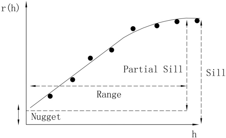
In the variogram model (Figure 2), spatial structures of geographical phenomena are mainly measured as nuggets, sills and ranges. The nugget is a random value reflected by spatial variability and measurement error.
Figure 2.
The variogram.
When the distance between sample points is approximately equal to zero, random error and spatial variability lead to variations in the variogram values, which will not be zero at the origin points. Range refers to the sample points within the range of spatial dependence. If the distance between two points is greater than the range, the sample point value differences will be stable. A sill is a platform value when the range is unchanged, and the sill is used to measure variation in an entire system.
2.3.2. Correlation Analysis of Spatial Risk Factors
Correlation analysis of spatial risk factors involves measuring and evaluating the correlations between a disease and its risk factors in a small area [7], and the general calculation for measuring risk factor and disease correlations is the Pearson correlation coefficient [33].
The Pearson correlation coefficient describes the degree of association between two variables. The coefficient is represented by the letter “r”, and the formula for the calculation is as follows:
| (3) |
where n is the sample number, and are the observed values of two variables, and are the averages of the two variables. R measures the degree of correlation between the two variables, and represents the standard deviations of the two variables. The value of r is between −1 and 1. If r > 0, there is a positive correlation between the two variables, whereas if r < 0, there is a negative correlation between the variables. For larger absolute values of r, there is greater correlation between the two variables. If r = 0, there is no linear correlation between the two variables.
As shown in Table 1, the interpretation of the Pearson correlation coefficient put forward by some scholars is as follows [34,35]. However, it should be noted that all of these criteria are, to a certain extent, arbitrary rather than strict [35]. The interpretation of correlation coefficients depends on the specific application background and purpose. Because the subject of this study was affected by various and complicated social factors, the requirements for the calculation results were not strict; thus, the criteria in the table can be considered reliable and reasonable.
Table 1.
Interpretation of the Pearson correlation coefficients.
| Correlation | Pearson Correlation Coefficient (Positive) | Pearson Correlation Coefficient (Negative) |
|---|---|---|
| Irrelevant | 0 to 0.09 | −0.09 to 0 |
| Weak correlation | 0.1 to 0.3 | −0.3 to −0.1 |
| Medium correlation | 0.3 to 0.5 | −0.5 to −0.3 |
| Strong correlation | 0.5 to 1.0 | −1.0 to −0.5 |
2.3.3. Analysis of Spatial Access
Spatial access is an uncertain concept that depends on specific occasions or practical problems [27]. In terms of this paper, spatial access was defined as the extent of overcoming spatial obstacles. Based on two groups of combination, potential and realized and spatial and non-spatial, access can be divided into four types: potential spatial access, potential non-spatial access, realized spatial access, realized non-spatial access [36]. Realized access refers to the actual consumption of services, whereas potential access refers to the possibility of service consumption. In this study, potential spatial access to medical resources was the study focus, because this form of access can evaluate whether the regional distribution of medical resources is reasonable.
In the study of spatial access to medical resources, there are mainly three factors: spatial distribution and the supply of medical services; spatial distribution and the residential area; and the spatial relationship between the population and medical services [27].
There are many methods for evaluating the spatial access. Generally speaking, the gravity model and the two-step floating catchment area method are extensively used in this field. This paper used the improved two-step floating catchment area method, which is different from the enhanced two-step floating catchment area method (E2SFCA, Luo W) [37], to measure the potential spatial interaction between patients and hospitals across administrative regions.
The improved two-step floating catchment area method is based on the method proposed by Radke and Mu but includes two improvements. First, the improved method considers the effect of distance decay in the search scope, thus overcoming the shortcoming that all of the demand points have the same access within the search scope. Second, the improved method offers an effective way to set the search radius for each hospital.
The improved two-step floating catchment area method includes the following two main steps, which are further elaborated:
(1) Setting the search radius value and calculating the ratio of supply and demand.
-
(a)
The search radius value can be set by the service level and capacity of each hospital. Hospitals are divided into three levels, with higher service levels, indicating a greater search radius value.
-
(b)
To set a more accurate hospital service radius, a group gradient search radius value can be set at the same hospital level. Each level has three search radius values.
-
(c)
Based on the requirements of the hospital, which mainly depend on the number of beds and the number of health technical personnel, each hospital’s service capacity can be calculated.
In sum, the hospital’s supply and demand ratio can be indicated by the following formula:
| (4) |
where is the hospital level, is the number of hospitals at that same level, is the number of study units, is the hospital’s service capacity and is the search radius. Each level has three search radius values. In addition, represents the distance between a residential area and a hospital, and is the population of each study unit.
(2) Calculating the spatial access in each study unit
To consider the effect of distance decay on search scope, a weight that is inversely proportional to the distance can be calculated according to the distance between residential areas and hospitals. The spatial access in each study unit, , can be indicated by the following formula:
| (5) |
where is the hospital level, is the number of hospitals at that same level, is the number of study units, is the hospital’s service capacity and is the search radius. Each level has three search radius values. In addition, represents the distance between a residential area and a hospital, and is the hospital level.
3. Results and Discussion
3.1. Spatial Distribution of Hepatitis B Morbidity in Shenzhen
3.1.1. Hepatitis B Data Processing
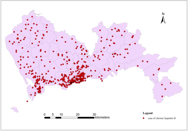
The statistical data for this paper included all new hospitalized hepatitis B cases in Shenzhen in 2010. In this group of data, there were 2,851 new hepatitis B cases. As shown in Figure 3, the distribution of hepatitis B cases was uneven, as cases were concentrated in the southwest of Shenzhen, but sparse in the rest of the city.
Figure 3.
Distribution of hepatitis B cases in Shenzhen in 2010.
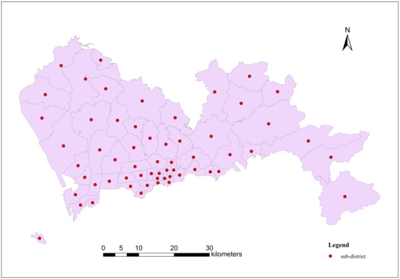
The home addresses of case were accurate to the sub-district level; as a result, geometric centre points of each sub-district could be used to represent respective spatial position (shown in Figure 4).
Figure 4.
The case data points in each sub-district.
These points represent the number of hepatitis B cases in each sub-district, as shown in Table 2. According to the table, Nantou, Lianhua and Yuehai demonstrated the most cases in Shenzhen in 2010.
Table 2.
The number of hepatitis B cases in each sub-district.
| Sub-District Name | Number of Cases | Sub-District Name | Number of Cases | Sub-District Name | Number of Cases |
|---|---|---|---|---|---|
| Shekou (N) | 7 | Dalang | 7 | Huangbei | 21 |
| Shekou (S) | 39 | Haishan | 1 | Liantang | 12 |
| Zhaoshang | 17 | Shatoujiao | 17 | Dongxiao | 6 |
| Nanshan | 9 | Meisha | 3 | Qingshuihe | 8 |
| Shahe | 21 | Yantian | 13 | Donghu | 37 |
| Nantou | 1443 | Shatou | 14 | Dapeng | 5 |
| Taoyuan | 4 | Nanyuan | 22 | Nanwan | 22 |
| Xili | 39 | Huaqiang North | 21 | Kuiyong | 5 |
| Yuehai | 74 | Xiangmihu | 15 | Buji | 73 |
| Longhua | 66 | Lianhua | 88 | Bantian | 18 |
| Xixiang | 57 | Yuanling | 10 | Henggang | 19 |
| Fuyong | 9 | HuaFu | 11 | Pingshan | 57 |
| Shiyan | 74 | Meilin | 40 | Pinghu | 48 |
| Shajin | 30 | Fubao | 7 | Longgang | 7 |
| Guangming (N) | 3 | Futian | 45 | Kengzi | 5 |
| Guangming (S) | 11 | Nanhu | 29 | Pingdi | 37 |
| Gongming | 50 | Guiyuan | 17 | Longcheng | 12 |
| Songgang | 38 | Dongmen | 13 | Nan’ao | 8 |
| Minzhi | 10 | Sungang | 8 | Xin’an | 15 |
| Guanlan | 39 | Cuizhu | 15 |
The raw statistical data based on the regional administrative units indicated the number of hepatitis B cases. These data were not suitable for spatial interpolation, but they can be converted to morbidity rates in epidemiological studies. The morbidity of hepatitis B was expressed as:
| (6) |
where M is the morbidity, is the number of new cases, and P is the exposed population.
In fact, with a larger population in a specific region, the morbidity from this calculation could be more accurate, and with a smaller population, the morbidity might be less accurate; thus, these morbidity data cannot reflect the true spatial distribution of hepatitis B. Based on the population in Shenzhen in 2010, there was a noticeable disparity among the different regions, making it necessary to adjust the morbidity in each sub-district to improve the accuracy.
Given that the true hepatitis B morbidity in one sub-district satisfying the normal distribution is a random variable, the hepatitis B morbidity obtained by calculation is only one instance of satisfying the normal distribution . Thus, more accurate hepatitis B morbidity can be determined using the Bayesian method and the results will be a linear combination of and [38]. The formulas are as follows:
| (7) |
| (8) |
where represents a weight with a value between 0 and 1, is population in each sub-district, represents mathematical expectation and represents variance of hepatitis B morbidity. The Equations (7) and (8) indicates that lower population leads to lower , and accounts for larger proportion of the weight, and is close to the . Conversely, is close to the .
The adjusted result of hepatitis B morbidity can be calculated using the Bayesian method with the mathematical expectation and variance of the normal distribution in each sub-district. The assessment of and is complex, whereas there is an easy way that the values of and in each sub-district are all the same to resolve this challenge, and thus and can be calculated using the number of new hepatitis B cases and the total population in each sub-district. The formulas are as follows:
| (9) |
| (10) |
where and represents the mean value of hepatitis B morbidity and population in the study area, respectively, and is the number of new hepatitis B cases in each sub-district.
Table 3 shows the adjusted hepatitis B morbidity in each sub-district, which was used for kriging interpolation after preprocessing. Before using kriging interpolation, morbidity data must be converted using a statistical method. Logarithmic conversion is widely used in this field, as it tends to shift data tend to a normal distribution and satisfy the data’s stationary hypothesis [39]. After the conversion, the morbidity data were in accordance with the demand of kriging interpolation.
Table 3.
The hepatitis B morbidity in each sub-district.
| Sub-District Name | Morbidity (104) | Sub-District Name | Morbidity (104) | Sub-District Name | Morbidity (104) | ||
|---|---|---|---|---|---|---|---|
| Shekou (N) | 1.56 | Dalang | 0.29 | Huangbei | 1.81 | ||
| Shekou (S) | 7.53 | Haishan | 0.33 | Liantang | 1.40 | ||
| Zhaoshang | 2.05 | Shatoujiao | 3.13 | Dongxiao | 0.67 | ||
| Nanshan | 0.64 | Meisha | 1.56 | Qingshuihe | 0.85 | ||
| Shahe | 1.70 | Yantian | 1.59 | Donghu | 4.06 | ||
| Nantou | 88.40 | Shatou | 0.65 | Dapeng | 1.12 | ||
| Taoyuan | 0.36 | Nanyuan | 1.97 | Nanwan | 1.13 | ||
| Xili | 2.04 | Huaqiang North | 3.49 | Kuiyong | 0.90 | ||
| Yuehai | 4.49 | Xiangmihu | 1.65 | Buji | 2.01 | ||
| Longhua | 1.78 | Lianhua | 5.01 | Bantian | 0.84 | ||
| Xixiang | 0.99 | Yuanling | 1.16 | Henggang | 0.64 | ||
| Fuyong | 0.22 | HuaFu | 1.53 | Pingshan | 2.70 | ||
| Shiyan | 2.92 | Meilin | 2.32 | Pinghu | 2.07 | ||
| Shajin | 0.58 | Fubao | 0.72 | Longgang | 0.37 | ||
| Guangming N) | 1.36 | Futian | 1.89 | Kengzi | 0.61 | ||
| Guangming (S) | 2.28 | Nanhu | 3.02 | Pingdi | 3.66 | ||
| Gongming | 1.21 | Guiyuan | 1.98 | Longcheng | 0.49 | ||
| Songgang | 0.96 | Dongmen | 1.43 | Nan’ao | 3.28 | ||
| Minzhi | 0.39 | Sungang | 1.27 | Xin’an | 0.39 | ||
| Guanlan | 0.87 | Cuizhu | 1.36 | ||||
3.1.2. The Spatial Distribution of Hepatitis B Morbidity
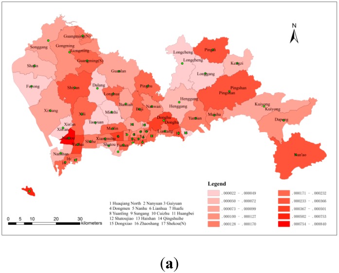
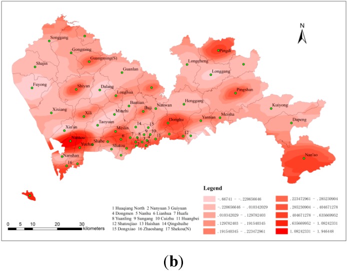
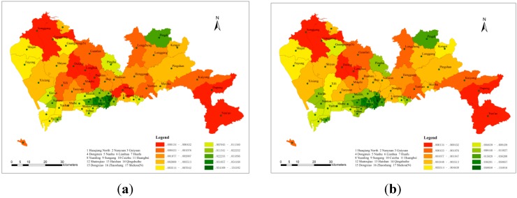
Figure 5 shows the spatial distribution of hepatitis B morbidity; Figure 5 used no interpolation method, whereas Figure 5b used kriging interpolation. In general, the locations of high morbidity on both graphs were the same, and the highest morbidity was observed in the southwest of Shenzhen. Nantou and its vicinity exhibited the most hepatitis B infections, and Guangming, Pingdi, Shiyan, Pingshan, Lianhua, Donghu, Nan’ao, Shekou (S) and their respective vicinities represented the other high-morbidity areas in Shenzhen in 2010. Comparing these two graphs, Figure 5a shows a statistical map of grade, whereas Figure 5 shows a contour map that weakens the influence of administrative boundaries on the spatial distribution of hepatitis B morbidity. The population often flows constantly from one district to another, and thus the results shown in Figure 5 better reflect the reality.
Figure 5.
(a) The spatial distribution of hepatitis B morbidity (non-interpolated) (b) The spatial distribution of hepatitis B morbidity (with kriging).
3.2. Spatial Risk Factor Analysis of the Spread of Hepatitis B
3.2.1. The Types of Risk Factors
The kriging interpolation results show that there were areas of high hepatitis B morbidity, and it can be inferred that some risk factors may have had an effect on this high morbidity. Hepatitis B is an infectious disease caused by HBV that is mainly transmitted through blood or body fluids. According to the conclusions of previous studies, some service facilities such as bath centres, beauty salons, massage parlours and pedicure parlours contribute to a high risk for HBV infection [40,41,42,43]. The shared utensils used at these facilities are not only unsterile, but also the skin of customers and service staff members can be easily broken during this services. Therefore, these four types of service facilities can be regarded as dangerous point sources of HBV infection.
3.2.2. Data Processing of Risk Factors
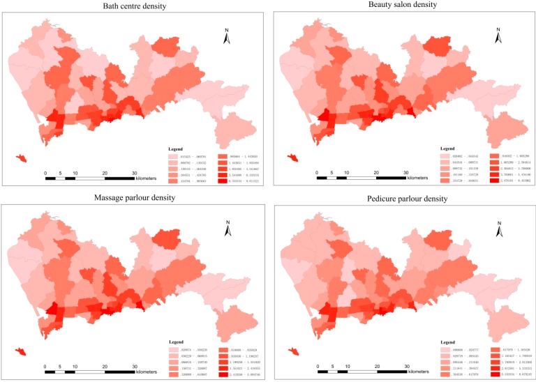
Data concerning the numbers and addresses for these four types of service facilities were extracted from Baidu maps. As shown in Figure 6, the spatial distribution of the four types of service facilities was uneven, with increasing numbers detected in southwest Shenzhen.
Figure 6.
The spatial distribution density of the four types of service facilities.
To accurately reflect the true spatial distribution of the four types of facilities, their density in each sub-district could be calculated with the following formula:
| (11) |
where is the density of the facilities in each sub-district, is the number of each type of facility in each sub-district, and S is the area of each sub-district.
Figure 6 shows the spatial distribution density of each type of service facility in each sub-district. The highest was observed in the south and southwest of Shenzhen. Comparing with Figure 5a,b and Figure 6, it is clear that there was a positive correlation between the hepatitis B morbidity distribution and the density distribution of the four types of service facilities. The correlation between these two factors could be measured accurately by calculating the Pearson correlation coefficient.
3.2.3. The Calculation and Explanation of the Pearson Correlation Coefficient
Table 4 shows the Pearson correlation coefficients calculated between each type of facility and the hepatitis B morbidity after performing a t-test (p < 0.05). In general, there was a positive correlation between these types of facilities and the hepatitis B morbidity, which suggests that these facilities have a positive effect on the spread of hepatitis B. Among the Pearson correlation coefficient results, the coefficient between massage parlours and hepatitis B morbidity was the largest of the four types of facilities, followed by bath centres, pedicure parlours and beauty salons.
Table 4.
Pearson correlation coefficients between hepatitis B morbidity and the type of service facility.
| Bath Centres | Beauty Salons | Massage Parlours | Pedicure Parlours |
|---|---|---|---|
| 0.566 | 0.515 | 0.626 | 0.538 |
Interpretation of the Pearson correlation coefficients is shown in Table 1. Because hepatitis B studies are related to the social sciences, the interpretation of coefficients in this table is considered to be reasonable and reliable. From the calculation results, each of the four types of service facilities showed a positive correlation with hepatitis B morbidity in Shenzhen in 2010. Although these four types of facilities to an extent can make people’s life convenient and drive local economic development, they greatly increase the risk of hepatitis B infection. Because of factors such as the large number of HBV-infected individuals in China, the troubling health status in the service facilities and a lack of disease prevention awareness, these four types of service establishment can be easily regarded as dangerous sources of HBV infection. Distinguishing between spatial risk factors not only helps to analyze how they influence the spatial spread of epidemic diseases, but also contributes to establishing disease prevention and control measures.
3.3. Analysis of Spatial Access to Medical Resources
3.3.1. The Spatial Distribution of Medical Resources
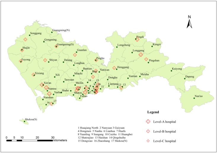
According to statistics from the Shenzhen Centre for Health Information, there were 139 hospitals in Shenzhen in 2010, and 65 hospitals with level certificates were related to the prevention and control of liver diseases. On the basis of the scale and level of medical treatment, the hospitals were divided into three levels in descending order: A, B and C. As shown in Figure 7, in terms of the number of hospitals, most hospitals were located in the southwest or south of Shenzhen. Specifically, there were 9 level-A hospitals, which have the largest red crosses; 22 level-B hospitals, with slightly smaller crosses; and 34 level-C hospitals, with the smallest crosses. Most of the hospitals with high service ability are also located in the southwest or south of Shenzhen. Thus, it can be concluded that Shenzhen lacks high-quality medical resources and that spatial distribution of medical resources is extremely uneven regardless of quantity or quality.
Figure 7.
Distribution of liver disease hospitals.
3.3.2. The Calculation of Spatial Access
The spatial access to medical resources was measured using the improved two-step floating catchment area method. The main calculation progress is described below:
1. Setting the value of the search radius
Based on the mean population density of Shenzhen and the number of people the hospitals provide with medical service [44], the search radius values for the different hospital levels were calculated. The result indicated that the level-A hospital search radius was 6 km, the level-B hospital search radius was 3 km, and the level-C hospital search radius was 1.7 km.
To more accurately determine the hospital service radius values, a group of gradient search radius values was set for the same hospital levels. Because Shenzhen lacked medical resources, the search radius value had to be somewhat larger. Therefore, for the level-A hospitals, the gradient search radius values were 6, 9 and 12 km; for the level-B hospitals, they were 3, 4 and 5 km and for the level-C hospitals, they were 1.7, 2 and 2.3 km.
2. Calculating the ratio of supply and demand
The calculation of spatial access to medical resources could be divided into three groups according to the different search radius values. Specifically, values of 6, 3 and 1.7 km, were used for the first group; 9, 4 and 2 km for the second group; and 12, 5 and 2.3 km for the third group.
Using the different search radius values for each group, search circles could be drawn using buffer analysis in ArcGIS Desktop (Environmental Systems Research Institute, Inc. [ERSI], Redlands, CA, USA). The number of points in the search circle was counted and the corresponding points in each sub-district were determined. Finally, each hospital’s supply and demand ratio was calculated using Equation (4).
3. Calculating the spatial access in each sub-district
Equation (5) uses two parameters: the distance between a residential area and a hospital, and each hospital’s level coefficient. The distance between the residential areas and hospitals was measured using the tools in ArcGIS. The hospital level coefficients, which were determined by hospital level, were 3, 2 and 1, corresponding to hospital levels A, B, and C. Then, spatial access to the hospitals in each sub-district could be calculated using Equation (5). However, some sub-districts may not have been included in any search circles; this would indicate that no services could be obtained for these sub-districts, which was highly unlikely. To resolve this challenge, we selected the nearest hospital to the sub-district and calculated its spatial access using the same process. Table 5 shows the spatial access to hospitals in each sub-district within different search radiuses.
Table 5.
Spatial access to hospitals in each sub-district within different search radiuses.
| Sub-District Name | Spatial Access to Hospitals at Different Search Radiuses (103) | ||
|---|---|---|---|
| 6, 3, 1.7 km | 9, 4, 2 km | 12, 5, 2.3 km | |
| Shekou (N) | 22.23 | 26.52 | 29.97 |
| Shekou (S) | 0.74 | 0.74 | 0.74 |
| Zhaoshang | 6.02 | 8.35 | 10.32 |
| Nanshan | 4.18 | 5.60 | 6.33 |
| Shahe | 2.30 | 5.64 | 9.26 |
| Nantou | 13.92 | 13.92 | 13.92 |
| Taoyuan | 1.49 | 2.76 | 7.24 |
| Xili | 0.67 | 4.09 | 4.77 |
| Yuehai | 7.04 | 8.44 | 9.93 |
| Longhua | 0.26 | 0.26 | 0.62 |
| Xixiang | 2.35 | 2.68 | 2.91 |
| Fuyong | 4.02 | 4.02 | 4.02 |
| Shiyan | 3.06 | 3.24 | 4.31 |
| Shajin | 4.35 | 4.35 | 4.35 |
| Guangming (N) | 3.05 | 3.05 | 3.05 |
| Guangming (S) | 6.02 | 6.02 | 6.02 |
| Gongming | 0.19 | 0.19 | 0.19 |
| Songgang | 0.43 | 0.43 | 0.43 |
| Minzhi | 0.82 | 1.48 | 2.50 |
| Guanlan | 0.70 | 0.70 | 0.70 |
| Dalang | 0.28 | 0.28 | 0.28 |
| Haishan | 11.34 | 11.34 | 13.46 |
| Shatoujiao | 5.95 | 5.95 | 9.24 |
| Meisha | 3.01 | 3.01 | 8.03 |
| Yantian | 1.08 | 1.08 | 1.08 |
| Shatou | 4.13 | 5.82 | 7.16 |
| Nanyuan | 20.63 | 24.50 | 25.40 |
| Huaqiang North | 51.10 | 58.86 | 60.84 |
| Xiangmihu | 7.82 | 14.52 | 19.33 |
| Lianhua | 30.58 | 31.72 | 31.72 |
| Yuanling | 29.13 | 35.10 | 36.31 |
| HuaFu | 54.17 | 57.96 | 58.23 |
| Meilin | 10.12 | 10.26 | 11.30 |
| Fubao | 9.60 | 12.30 | 12.30 |
| Futian | 8.31 | 10.47 | 10.47 |
| Nanhu | 42.56 | 46.43 | 47.67 |
| Guiyuan | 31.86 | 36.20 | 36.20 |
| Dongmen | 47.61 | 49.84 | 49.84 |
| Sungang | 42.51 | 46.05 | 47.65 |
| Cuizhu | 154.18 | 155.82 | 156.69 |
| Huangbei | 16.49 | 20.47 | 21.82 |
| Liantang | 3.51 | 3.51 | 7.98 |
| Dongxiao | 16.23 | 21.64 | 23.67 |
| Qingshuihe | 14.37 | 15.03 | 17.70 |
| Donghu | 0.20 | 2.76 | 6.57 |
| Dapeng | 0.13 | 0.13 | 0.13 |
| Nanwan | 1.60 | 3.22 | 4.67 |
| Kuiyong | 0.62 | 0.62 | 0.62 |
| Buji | 2.01 | 3.15 | 4.10 |
| Bantian | 0.38 | 1.58 | 2.89 |
| Henggang | 1.85 | 1.85 | 1.85 |
| Pingshan | 2.67 | 2.67 | 2.67 |
| Pinghu | 11.06 | 11.06 | 11.48 |
| Longgang | 1.77 | 2.82 | 2.82 |
| Kengzi | 2.49 | 4.64 | 4.64 |
| Pingdi | 24.79 | 26.83 | 26.83 |
| Longcheng | 0.60 | 0.60 | 1.11 |
| Nan’ao | 0.40 | 0.40 | 0.40 |
| Xin’an | 10.16 | 10.16 | 10.16 |
4. Kriging interpolation of spatial access
Kriging interpolation can also be used to determine the spatial access to medical resources. Using the same method of logarithmic conversion, the spatial access data for each sub-district were transformed to approximate the normal distribution and satisfy the stationary data hypothesis.
3.3.3. The Distribution of Spatial Access
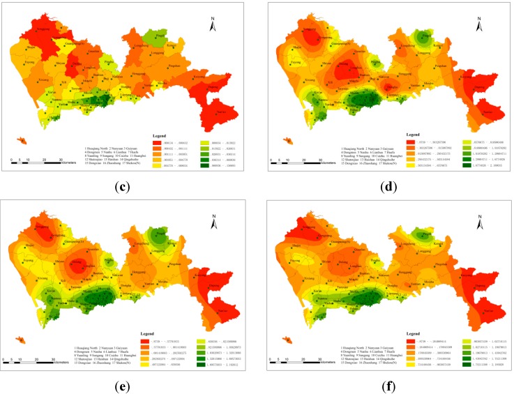
Figure 8a–c shows the spatial access in each sub-district, without interpolation, in the three different search radius groups. The search radius values in Figure 8a were 6, 3 and 1.7 km, corresponding to hospital levels A, B, and C, respectively. Similarly, the values in Figure 8b,c were 9, 4, 2 km and 12, 5, 2.3 km, respectively. These values showed the same corresponding relationship with hospital level. Within the three groups, Cuizhu, Huaqiang North and Huafu were the sub-districts with the most spatial access. Figure 8d–f shows three contour maps, for which kriging interpolation was used, that were also based on the different search radius values. The locations of high and low spatial access were approximately the same, and the distribution of access was uneven as well. In general, there were three centres with high spatial access, which were concentrated in the southwest, south and northeast, and two low-access centres, which were concentrated in the northwest and southeast. The reason for this distribution pattern is that most of the high-quality medical resources are concentrated in the southern area, which is the economic centre of Shenzhen. In addition, most of the level-A hospitals which have sufficient paramedics, advanced medical facilities, and professional medical staff, are located in the same region, whereas in areas with low spatial access, there is a lack of medical resources to meet the demands of the surrounding population.
Figure 8.
The spatial access in each sub-district. (a) 6, 3, 1.7 km (non-interpolated); (b) 9, 4, 2 km (non-interpolated); (c) 12, 5, 2.3 km (non-interpolated); (d) 6, 3, 1.7 km (with kriging); (e) 9, 4, 2 km (with kriging); (f) 12, 5, 2.3 km (with kriging).
3.3.4. Relationship between Hepatitis B Morbidity and Spatial Access
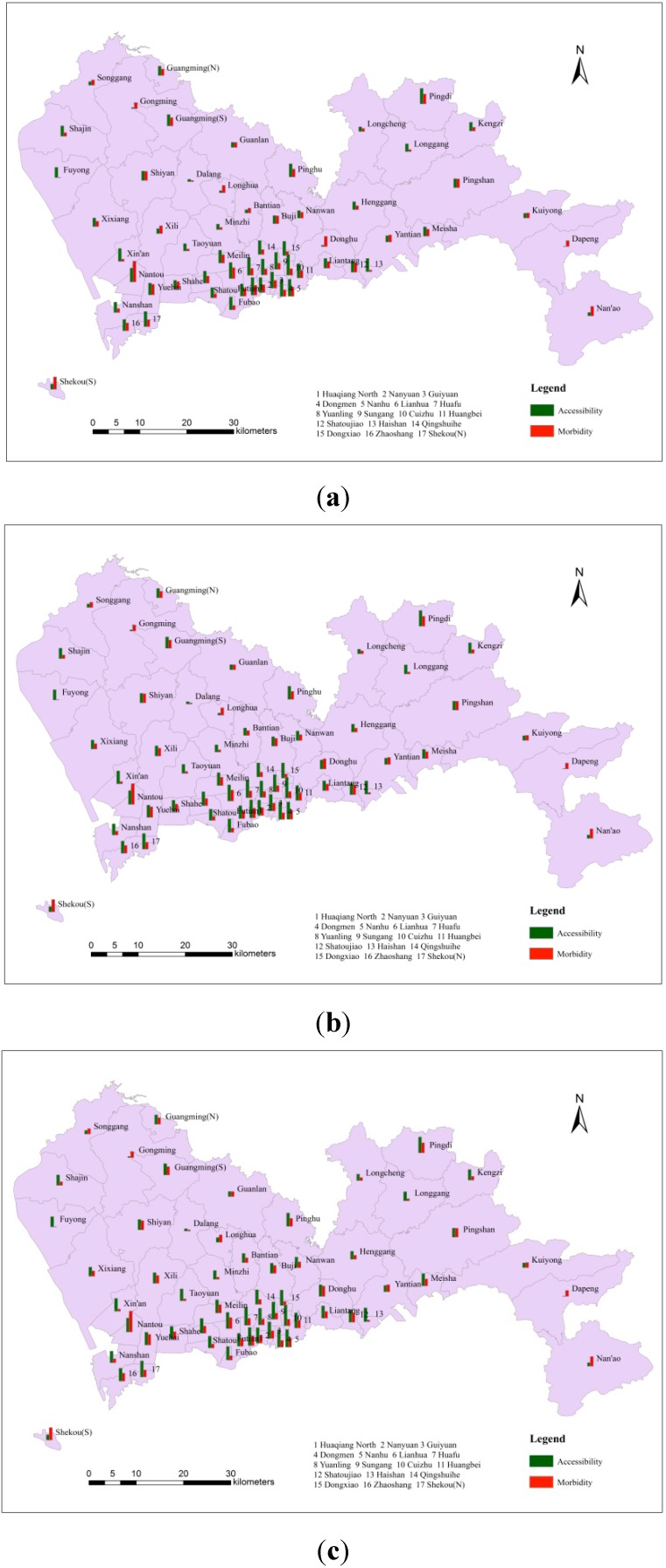
The adequacy of medical resources can be measured by the spatial access index, and comparing a patient’s regional access to medical resources with disease morbidity make it possible to determine whether the regional medical resource distribution is adequate for this particular disease. In Figure 9, the green column represents access to regional medical resources, and the orange column represents hepatitis B morbidity. It can be seen from these three figures that regardless of the search radius, in sub-districts with high hepatitis B morbidity, the spatial access index was generally higher; whereas in sub-districts with low morbidity, the spatial access index was generally lower. This result indicated that hospitals were able to provide sufficient medical services for neighbouring hepatitis B patients. In general, the allocation and spatial distribution of medical resources for hepatitis B were adequate.
Figure 9.
The comparison between spatial access and hepatitis B morbidity. (a) Search radiuses: 6, 3, 1.7 km; (b) Search radiuses: 9, 4, 2 km; (c) Search radiuses: 12, 5, 2.3 km.
4. Conclusions
1. In epidemiological research, mining geographic spatial data can not only reveal the spatial distribution characteristics of infectious diseases but also may identify risk factors that have a major impact on the spread of these diseases. In addition, assessing the spatial access to medical resources can reveal the accuracy of medical resource spatial distribution. These studies have important significance for establishing infectious disease prevention and control measures.
2. The spatial distribution of hepatitis B; the distribution of high-transmission-risk facilities such as bath centres, beauty salons, massage parlours and pedicure parlours and access to regional medical resources were uneven in Shenzhen in 2010, with a main concentration of such factors in the south and southwest, which correspond to the economic centre regions of Shenzhen. On the one hand, these distribution characteristics indicated that hepatitis B infection had a positive correlation with the four high-risk service facilities. On the other hand, the allocation and spatial distribution of medical resources for hepatitis B was adequate.
3. In view of these conditions, measures must be taken to strengthen the prevention and control of hepatitis B, such as improving the sanitary conditions in service facilities, raising awareness about the spread and prevention of hepatitis B and strengthening the construction of medical facilities in economically less-developed areas in Shenzhen.
4. This paper did not research spatial distribution of hepatitis B in a temporal manner because of limited data. In addition, the correlation between hepatitis B and high-risk locations was not very strong, and thus further studies are necessary to determine whether hepatitis B correlates with certain geographical or other elements in Shenzhen city. Furthermore, The method, the improved two-step floating catchment area model to evaluate the spatial access to medical resources must continuously be modified for more accurate evaluation results. These limitations will be studied further in the future.
Acknowledgments
We thank Ke Xiao, Sheng Li, Ruichang Li and Jie Lian, Miss Langjiao Li for their help. In addition, this study was supported by the National Natural Science Foundation of China (Project No.41271455/D0108) and the Fundamental Research Funds for the Central Universities (Project No.2042014KF0282). This study was also supported by the Government Support Item Foundation of Shenzhen (Project No. 201201017 major project, Medical and Health Care Class; Project No. JCYJ20130329164302637).
Author Contributions
All of the authors contributed to this study. Specifically, Yu-Liang Xi and Jinghua Zhang conducted the primary experiments, cartography and analysis of the results. Fu Ren introduced the idea, organized the content, and provided research funding for the study. Shi Liang provided insight for the analysis of Hepatitis B Disease (HBD) and the prediction of HBD. De-nan Lin collected all the data of HBD in Shenzhen in 2010 and preprocessed them. Yu-Liang Xi wrote the manuscript.
Conflicts of Interest
The authors declare no conflict of interest.
References
- 1.Shahnaz S., Seyed M.A., Graham R.F. Influencing factors on the outcome and prognosis of patients with HBV infection: Seven years follow-up. Hepat. Mon. 2013;13:1–7. doi: 10.5812/hepatmon.8743. [DOI] [PMC free article] [PubMed] [Google Scholar]
- 2.Lu F.M., Zhuang H. Prevention of hepatitis B in China: Achievements and challenges. Chinese Med. J. 2009;122:2925–2927. [PubMed] [Google Scholar]
- 3.Zhang Y., Zhang H., Elizabeth A. Epidemiology of hepatitis B and associated liver diseases in China. Chinese Med. Sci. J. 2012;27:243–248. doi: 10.1016/s1001-9294(13)60009-7. [DOI] [PubMed] [Google Scholar]
- 4.Tanaka M., Katayama F., Kato H. Hepatitis B and C virus infection and hepatocellular carcinoma in China: A review of epidemiology and control measures. Epidemiology. 2011;21:401–416. doi: 10.2188/jea.JE20100190. [DOI] [PMC free article] [PubMed] [Google Scholar]
- 5.Statistical Methods in Spatial Epidemiology. [(accessed on 22 October 2011)]. Available online: https://www.jstage.jst.go.jp/article/jea/21/6/21_JE20100190/_article.
- 6.Pfeiffer D., Robinson T., Stevenson M. Spatial Analysis in Epidemiology. Oxford University Press; New York, NY, USA: 2008. [Google Scholar]
- 7.Zhou X.N. Spatial Epidemiology. Science Press; Beijing, China: 2009. [Google Scholar]
- 8.Wang Z.S., Du Q.Y., Liang S. Analysis of the spatial variation of hospitalization admissions for hypertension disease in Shenzhen, China. Int. J. Environ. Res. Public Health. 2014;11:713–733. doi: 10.3390/ijerph110100713. [DOI] [PMC free article] [PubMed] [Google Scholar]
- 9.Hu T., Du Q.Y., Liang S. Spatial analysis of the home addresses of hospital patients with hepatitis B infection or hepatoma in Shenzhen, China from 2010 to 2012. Int. J. Environ. Res. Public Health. 2014;11:3143–3155. doi: 10.3390/ijerph110303143. [DOI] [PMC free article] [PubMed] [Google Scholar]
- 10.Wang Y.X., Du Q.Y., Ren F. Spatio-temporal variation and prediction of ischemic heart disease hospitalizations in Shenzhen, China. Int. J. Environ. Res. Public Health. 2014;11:4799–4824. doi: 10.3390/ijerph110504799. [DOI] [PMC free article] [PubMed] [Google Scholar]
- 11.Elliott P., Wartenberg D. Spatial epidemiology: Current approaches and future challenges. Environ. Health Perspect. 2004;112:998–1006. doi: 10.1289/ehp.6735. [DOI] [PMC free article] [PubMed] [Google Scholar]
- 12.Guo R.Z. Spatial Analysis. China Higher Education Press; Beijing, China: 2011. [Google Scholar]
- 13.Cliff A., Haggett P., Du C.Z. Disease mapping. Prog. Geog. 1990;9:44–49. [Google Scholar]
- 14.Lu B.L., Wang J.F., Zeng G. Approaches to study disease clustering in space. Dis. Surveill. 2010;25:394–396. [Google Scholar]
- 15.Lynch M., Painter J., Woodruff R. Surveillance for foodornborne-disease outbreaks—United States, 1998–2002. Surveill. Summ. 2006;55:1–42. [PubMed] [Google Scholar]
- 16.Kulldorff M., Nagarwalla N. Spatial disease clusters: Detection and inference. Stat. Med. 1995;14:799–810. doi: 10.1002/sim.4780140809. [DOI] [PubMed] [Google Scholar]
- 17.Kulldorff M. A spatial scan statistic. Commun. Stat. Theory Methods. 1997;26:1481–1496. doi: 10.1080/03610929708831995. [DOI] [Google Scholar]
- 18.Li X.Z., Wang J.F. A fast method for making candidate clusters in spatial scan statistic method. J. Geoinf. Sci. 2013;15:505–511. [Google Scholar]
- 19.Muhoho N.D., Katsumata T., Kimura E. Cercarial density in the river of an endemic area of schistosomiasis haematobia in Kenya. Am. J. Trop Med. Hyg. 1997;57:162–167. doi: 10.4269/ajtmh.1997.57.162. [DOI] [PubMed] [Google Scholar]
- 20.Zhang Z.J. Spatial Analysis on the High Risk Regions for Schistosomiasis Japonnica and Identification of Active Transmission Sites. Fudan University; Shanghai, China: 2010. [Google Scholar]
- 21.Zhang A., Qi Q.W., Jiang L.L. Population exposure to PM2.5 in the urban area of Beijing. PLoS One. 2013;8 doi: 10.1371/journal.pone.0063486. [DOI] [PMC free article] [PubMed] [Google Scholar]
- 22.Liu X.T. General description of spatial accessibility. Urban Transport. China. 2007;5:36–43. [Google Scholar]
- 23.Li P.H., Lu Y.Q. Review and prospect of accessibility research. Progr. Geogr. 2005;24:69–78. [Google Scholar]
- 24.Joseph AE., Phillips D.R. Accessibility and Utilization: Geographical Perspectives on Health Care Delivery. Sage Publications Ltd.; London, UK: 1984. [Google Scholar]
- 25.Radke J., Mu L. Spatial decompositions, modeling and mapping service regions to predict access to social programs. Geogr. Infor. Sci. 2000;6:105–112. [Google Scholar]
- 26.Hu R.S., Dong X.C., Hu H. A two-step floating catchment area (2SFCA) method for measuring spatial accessibility to primary healthcare service in China: A case study of Donghai County in Jiangsu Province. Progr. Geogr. 2012;31:1600–1607. [Google Scholar]
- 27.Qu R. Research on Spatial Patterns of Epidemic Disease Based on Spatial Data Analysis: In Hepatitis B Disease as An Example. Wuhan University; Wuhan, China: 2013. [Google Scholar]
- 28.National Bureau of Statistics of the People’s Republic of China . Major Figures on 2010 Population Census of China. China Statistics Press; Beijing, China: 2011. [Google Scholar]
- 29.Paul AL., Michael F.G., David J.M. Geographical Information Systems and Science 2nd Edition. Wiley; New York, NY, USA: 2004. [Google Scholar]
- 30.Wu L., Liu Y., Zhang J. The Principle, Method and Application of Geographic Information System. Science Press; Beijing, China: 2005. [Google Scholar]
- 31.Li J.X., Li C.K., Yin Z.H. ArcGIS based kriging interpolation method and its application. Bull. Surv. Mapp. 2013;9:87–90. [Google Scholar]
- 32.Liu A.L., Wang P.F., Ding Y.Y. Introduction to Geostatistics. Science Press; Beijing, China: 2012. [Google Scholar]
- 33.Cao Z.D., Wang J.F., Gao Y.H. Risk factors and autocorrelation characteristics on severe acute respiratory syndrome in Guangzhou. J. Geogr. Sci. 2008;63:981–993. [Google Scholar]
- 34.Buda A., Jarynowski A. Life-time of correlations and its applications. Wydawnictwo Niezalezne. 2010;1:5–21. [Google Scholar]
- 35.Cohen J. Statistical Power Analysis for the Behavioral Sciences. 2nd ed. Routledge; London, UK: 1988. [Google Scholar]
- 36.Khan A.A. An integrated approach to measuring potential spatial access to health care services. Socioecon. Plann. Sci. 1992;26:275–287. doi: 10.1016/0038-0121(92)90004-O. [DOI] [PubMed] [Google Scholar]
- 37.Luo W., Qi Y. An enhanced two-step floating catchment area (E2SFCA) method for measuring spatial accessibility to primary care physicians. Health Place. 2009;15:1100–1107. doi: 10.1016/j.healthplace.2009.06.002. [DOI] [PubMed] [Google Scholar]
- 38.Cao Z.D., Zeng D.J., Zheng X.L. Spatio-temporal evolution of Beijing 2003 SARS epidemic. Sci. China Earth Sci. 2010;40:776–788. doi: 10.1007/s11430-010-0043-x. [DOI] [PMC free article] [PubMed] [Google Scholar]
- 39.Zhong S.B. Application of GIS and Remote Sensing for Study of Epidemiology of Infectious Disease-Case Studies of Hepatitis B and Highly Pathogenic Avian Influenza. Academy of Science; Beijing, China: 2010. [Google Scholar]
- 40.Chen Y.S. Study of the risk of HBV Infection in the Public Service Place. Chinese Center for Disease Control and Prevention; Beijing, China: 2009. [Google Scholar]
- 41.Wen G.Y., Chen H.P., Liu Y. Investigation and analysis on risk factors of hepatitis B transmission in public places in Xining City. Chin. Prim. Health Care. 2009;23:69–70. [Google Scholar]
- 42.Song D.H., Zhang S.R., Zhao J.H. The knowledge, attitude and behavior on hepatitis B prevention between hepatitis B patients and healthy people. Mod. Prevent. Med. 2009;36:688–691. [Google Scholar]
- 43.Chen Y.S., Zhou Y.Q., Wang X.J. Study on the status sanitizing and HBV contamination of appliances used in the public service places. Chin. J. Vaccines Immun. 2008;14:315–318. [Google Scholar]
- 44.Shenzhen Statistics and Information Bureau . Shenzhen Statistical Yearbook 2010. China Statistics Press; Beijing, China: 2011. [Google Scholar]


