Multivariate Genetic Analysis of Sex Limitation and G × E Interaction

Abstract

Sex-limited expression of genetic or environmental factors occurs in two basic forms. First, the effects of a factor may be larger on one sex than on another, which is known as scalar sex limitation. Second, some factors may have an effect on one sex but not on the other, which is called nonscalar sex limitation. In the classical twin study, scalar sex-limited effects cause same-sex male and same-sex female twin correlations to differ. Nonscalar sex-limited effects would cause the correlations between opposite-sex pairs of relatives to be lower than would be expected from the correlations between relatives of the same sex. One approach to modeling such effects is to allow the genetic correlation between opposite-sex dizygotic twins to be less than one-half; another is to allow the common environment correlation for opposite-sex pairs to be less than unity. Extension of this approach to the multivariate case is not straightforward. Direct extension of the Cholesky decomposition such that each Cholesky factor is allowed to correlate less than one-half in opposite-sex pairs yields a model where the order of the variables can change the goodness-of-fit of the model. It is shown that similar problems exist with a variety of multivariate and longitudinal models, and in a variety of models of genotype × environment interaction. Several solutions to these problems are described.

Sex limitation has long been a focus of quantitative genetic studies in both animals and plants (Mather & Jinks, 1977). It occurs when the effects of genetic or environmental factors differ between males and females. Two forms of sex limitation are generally considered. First is scalar sex limitation, where the differences are purely quantitative, in that the same factors affect both sexes, but their impact on the phenotype is greater in one sex than the other. Scalar sex limitation of genetic factors alone will cause the covariances between biological relatives to differ between females and males. In terms of a statistical model, the regression coefficient of the phenotype on the standardized (unit variance) genotype for males, which we term a_m, would not equal that for females, a_f. Under scalar sex limitation, the genetic covariance between dizygotic (DZ) male twin pairs is $.5a_m^{\mathit{2}}$, between DZ female pairs it is $.5a_f^{\mathit{2}}$, and between opposite-sex pairs it is predicted to be the geometric mean of these quantities, .5a_fa_m. Second is nonscalar sex limitation, which is qualitative, such that there exist one or more factors that influence trait variation in one sex but not the other. Both scalar and nonscalar sex limitation are a specific form of heterogeneity model; other forms subsume models of genotype × environment interaction.

Models for sex limitation in outbred populations such as humans have been available for decades (Eaves et al., 1978), and practical methods for fitting such models in the univariate case are well-known (Neale & Cardon, 1992). Although extensions to the multivariate case have been presented elsewhere (Maes et al., 1999; Neale et al., 1994), these accounts are limited in that they do not consider difficulties with the application of the Cholesky decomposition to multivariate sex limitation. The goals of this article are to identify the cause of these problems, and to provide solutions that circumvent them.

Univariate Models of Sex Limitation: The Twin Study

In the context of the classical twin study, it is possible to estimate components of variance, such as additive genetic (A), specific environment (E), and either dominance (D) or common environment (C). These estimates could be obtained for male–male and female–female twin pairs and the results could be ‘eyeballed’ for differences. This simple approach has at least three serious limitations (Neale & Cardon, 1992): it does not have a statistical assessment of the magnitude of the differences; it omits opposite-sex twin pairs; and it does not discriminate between types of sex limitation.

Data from DZ opposite-sex twin pairs (DZOS) provide the information to estimate a reduced additive genetic correlation for opposite-sex pairs, such that their predicted genetic covariances of .5a_ma_f becomes .5r_gmfa_ma_f, where r_gmf is the correlation between the additive genetic factors in males and those in females. However, DZOS do not provide sufficient information to estimate an additional parameter for reduced correlation between genetic dominance factors (r_d), nor for reduced correlation between their common environment factors (r_c). The absence of opposite-sex monozygotic (MZ) twins precludes the estimation of these additional parameters. The DZ opposite-sex pairs effectively provide only one new statistic, their covariance, which provides the information to estimate one and only one new parameter. Other research designs, such as the study of the offspring of MZ and DZ twins, permit simultaneous estimation of more than one parameter for reduced genetic and environmental correlation. No reduced correlation for specific environmental factors can be estimated, because these are assumed to be uncorrelated between the members of twin pair.

It should be noted that while the context of the present discussion is sex limitation, the arguments apply equally to gene × gene, gene × environment, or environment × environment interaction. For example, twin pairs might be grouped according to their exposure to a stressor, in which case we could see six types of twin pair, MZ or DZ by concordant exposed, concordant unexposed, or discordant exposed. The following discussion concerning the use of the Cholesky decomposition for multivariate analysis of sex limitation applies equally to multivariate models of gene × environment or environment × environment interaction.

Multivariate Genetic Models

Early accounts of multivariate genetic analysis of data collected from human twin pairs focused on the estimation of genetic and environmental correlation and covariance matrices (Martin & Eaves, 1977; Vandenberg, 1965). Analyses of this type provided a ‘Gestalt’ impression of the degrees of genetic and environmental communality between traits. In a second step, exploratory factor analysis was sometimes used to examine the factor structure of these genetic and environmental covariance matrices. However, as pointed out by Martin and Eaves (1977), two-stage analysis of this sort has the problem that it makes testing hypotheses about the number of factors difficult because the precision of the correlations in a genetic correlation matrix is not readily available. This problem led to the development of modeling methods in which the genetic and environmental factors were specified directly during the model-fitting process. Effectively, the confirmatory factor analysis approach in which a factor pattern is pre-specified and fitted to the observed data, has replaced the exploratory approach, where the factor structure is surmised from inspection of the estimates of factor loadings under a generic model. This change of emphasis has occurred in both genetic and nongenetic modeling of covariance structure.

In this article, we wish to consider the case of a saturated model for genetic covariances in the sex-limited case. Our focus should not be taken to imply that saturated models for genetic covariances are the best, or that we are recommending a strategy of estimating these statistics and subsequently conducting exploratory factor analyses or otherwise drawing conclusions from their inspection. The estimation of this saturated model has a different purpose, which is to provide a baseline model against which the fit of alternative genetic factor models can be compared. A second use of the saturated model for sex limitation is to provide a multivariate test, which, if significant, would justify testing for sex limitation in one or more members of the set of traits in the multivariate analysis.

A technical problem with estimating genetic covariance matrices is that it is desirable to restrict the solutions to those that are realistic. Several issues must be considered when generating covariance matrices, and these issues are slightly different for component covariance matrices (additive genetic, specific environment, etc.) than for the phenotypic covariance matrix that results from their sum. First, any process that causes individual differences, be it the effects of a locus on mean values of a phenotype, or the effects of environmental conditions on the same, must cause a positive amount of variance in the phenotypes. Second, it will not be possible for these processes to produce a predicted correlation between two phenotypes that is greater than unity. Third, it should not be possible to generate correlation matrices that are inconsistent, for example if A correlates 1.0 with B, the correlation between A and C must equal the correlation between B and C. Fourth, the predicted phenotypic covariance matrix (formed by the sum of the genetic and environmental covariance matrices) must be positive definite (see Appendix 1 for definition).

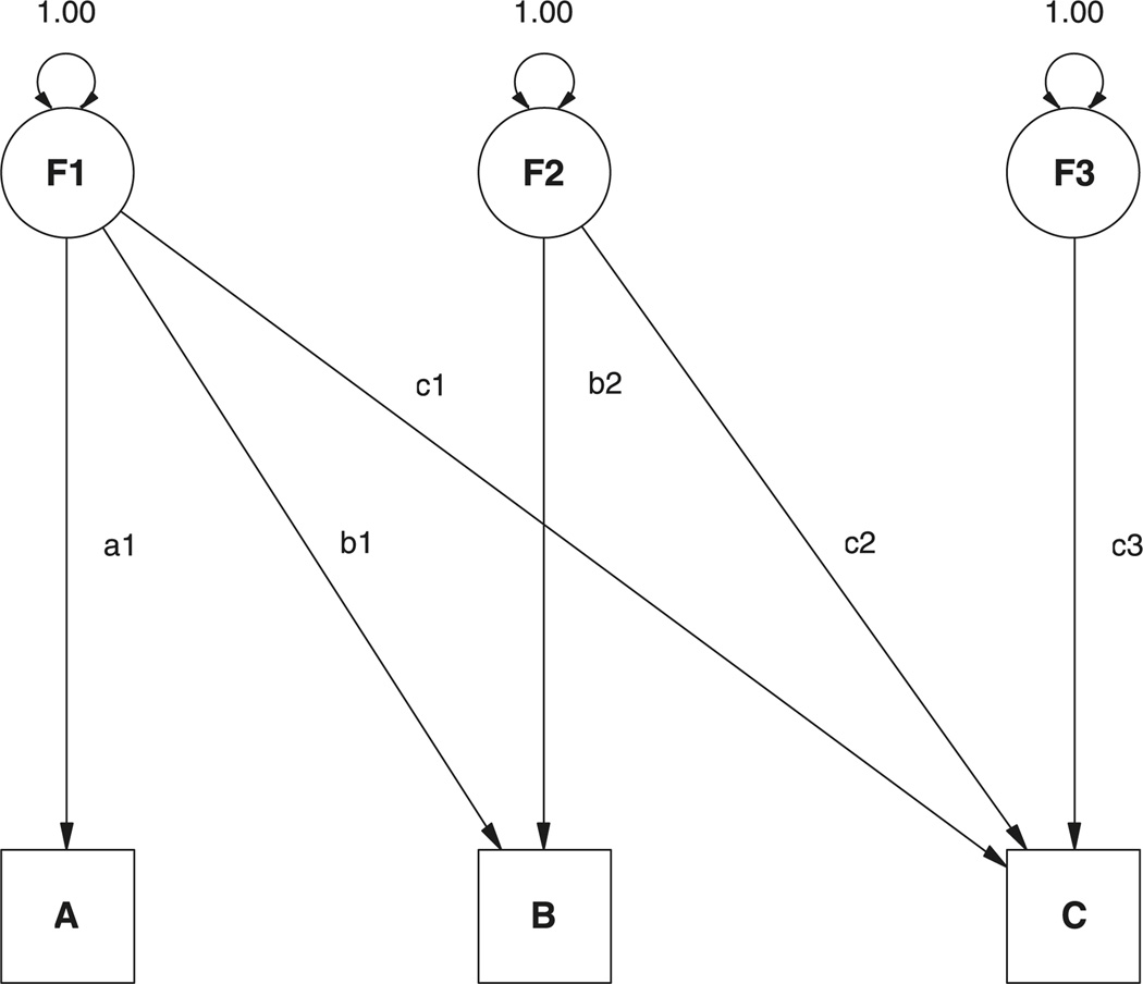
All four of the above restrictions are imposed if the genetic and common environmental covariance matrices are constrained to be nonnegative definite, and the specific environment covariance matrix is constrained to be positive definite (see Appendix A for proof). The Cholesky or triangular decomposition provides a convenient way to impose these constraints. This approach may be regarded as factor model (see Figure 1), in which each of the observed variables P_j, j = 1…m has a corresponding factor F_j. Each factor F_j may influence only variables P_j to P_m. A great advantage of this Cholesky factor decomposition is that it imposes the positive semi-definite constraint (see Appendix A, Theorem 1 for proof). A genetic model for the covariance of phenotypes is usually formed from the sum of several such matrices, for example, V_P = V_A + V_C + V_E, which will also be positive semi-definite. To make the predicted phenotypic covariance matrix V_P strictly positive definite, it is sufficient to ensure that the specific environment matrix is positive definite and that the additive genetic and common environmental matrices (V_A and V_C) are nonnegative definite. This is a reasonable constraint to impose because the specific environment matrix includes the effects of measurement error, at least part of which may be assumed to generate at least some variable-specific variance. The proof of Theorem 2 in Appendix A shows that by constraining the diagonal elements of the Cholesky factor matrix to be greater than zero, the resulting covariance matrix will be positive definite. We note here that imposing constraints of this sort can give rise to statistical problems, as discussed by Carey (2005). These ‘Cholesky’ problems are not the focus of this article, though we return to consider their implications in the discussion.

Figure 1.

Cholesky decomposition as a structural equation model.

Problems With the Cholesky Decomposition

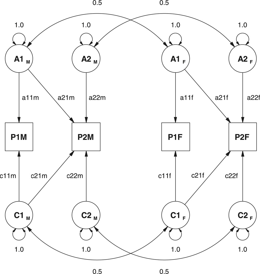
Modeling scalar sex limitation might appear to be straightforward for the multivariate case. A five-group structural equation model can be constructed, in which latent variables are sex-specific, so that paths to male twin phenotypes are allowed to differ from those to female twin phenotypes. One approach to this model is shown in Figure 2. Here the genetic covariance between the traits is modeled as a bivariate Cholesky or triangular decomposition. This formulation partitions the genetic factors into two components: those that are common to both traits, and those that are specific to the second trait. The choice of which trait is first should be arbitrary, in that either order would produce the same fit to the data. It does so when data from same-sexed relatives alone are analyzed.

Figure 2.

Path diagram for a model of sex limitation in a pair of DZ opposite-sex twins, using a Cholesky factor approach. Only the phenotypes P1_s, additive genetic factors, A1_s, and common environment factors, C1_s, are shown, in which 1 refers to trait 1 and subscript s refers to the sex of the twin.

There is, however, a serious problem with this model.

The essential idea of the scalar sex-limitation model is that the same factors cause variation in males and females, but that they do so to a different extent. Indeed, we might suppose that these factors only differ in mean and variance between the sexes, in accordance with a measurement invariance model (Lubke et al., 2004; Meredith, 1993). Since the factors are the same in males and females, they must covary with each other to the same extent. In other words, the model requires that there is only one common factor correlation structure, R_A, but different loadings on these factors for males and females.

It might be thought that a generalization of the Cholesky approach for sex limitation would involve defining lower triangular matrices, X_M and X_F, to decompose the additive genetic covariances for males (A_M = X_MX_M) and females (A_M = X_FX_F). The opposite-sex dizygotic genetic covariance would then be estimated as .5⊗X_FX_M. However, this model does not retain the required constraint for scalar sex limitation that the factors correlate equally in males and females.

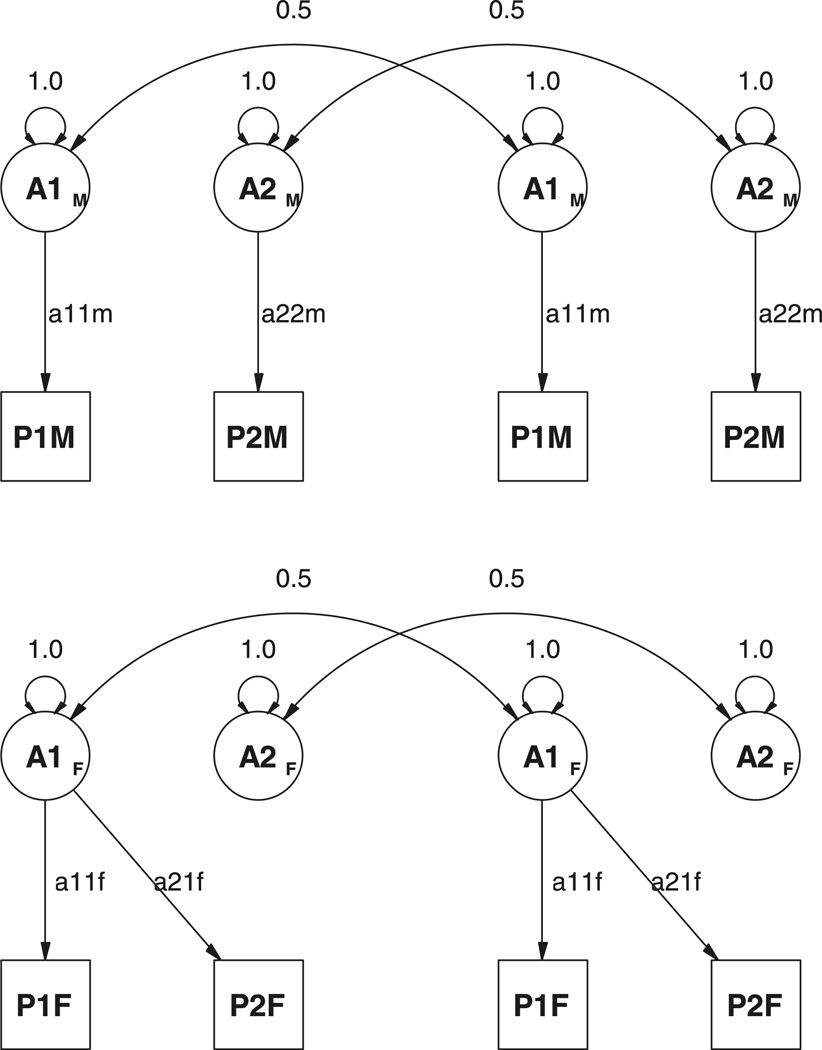
An additional problem for the purposes of applied data analysis is that the overall fit of the model will depend on the order of the variables in the analysis. This property is easy to demonstrate with a simple example. Suppose that a bivariate Cholesky model is fitted to data from male twin pairs, and it is found that there is genetic variance of 1.0 for both traits, but zero genetic covariance between them. Also suppose that the same analysis is performed for female twin pairs, and that although the same genetic variance of 1.0 is found, the genetic covariance is 1.0 instead of zero. This situation is illustrated in Figure 3. In terms of model parameters, the estimates of the male Cholesky matrix are:

$$\mathbf{X}=\left[\begin{array}{cc}\hfill a\hfill & \hfill 0\hfill \\ \hfill b\hfill & \hfill c\hfill \end{array}\right]=\left[\begin{array}{cc}\hfill 1\hfill & \hfill 0\hfill \\ \hfill 0\hfill & \hfill 1\hfill \end{array}\right]$$

and those of the females are

$$\mathbf{Y}=\left[\begin{array}{cc}\hfill d\hfill & \hfill 0\hfill \\ \hfill e\hfill & \hfill f\hfill \end{array}\right]=\left[\begin{array}{cc}\hfill 1\hfill & \hfill 0\hfill \\ \hfill 1\hfill & \hfill 0\hfill \end{array}\right]$$

If the predicted covariance matrix between opposite-sex twin pairs is set to equal X(.5⊗IY′) then we obtain the following:

$$\mathbf{X}.5\otimes \mathbf{I}\mathbf{Y}\prime =\left[\begin{array}{cc}\hfill ad\hfill & \hfill ae\hfill \\ \hfill bd\hfill & \hfill be+cf\hfill \end{array}\right]=\left[\begin{array}{cc}\hfill 1\hfill & \hfill 1\hfill \\ \hfill 0\hfill & \hfill 0\hfill \end{array}\right]$$

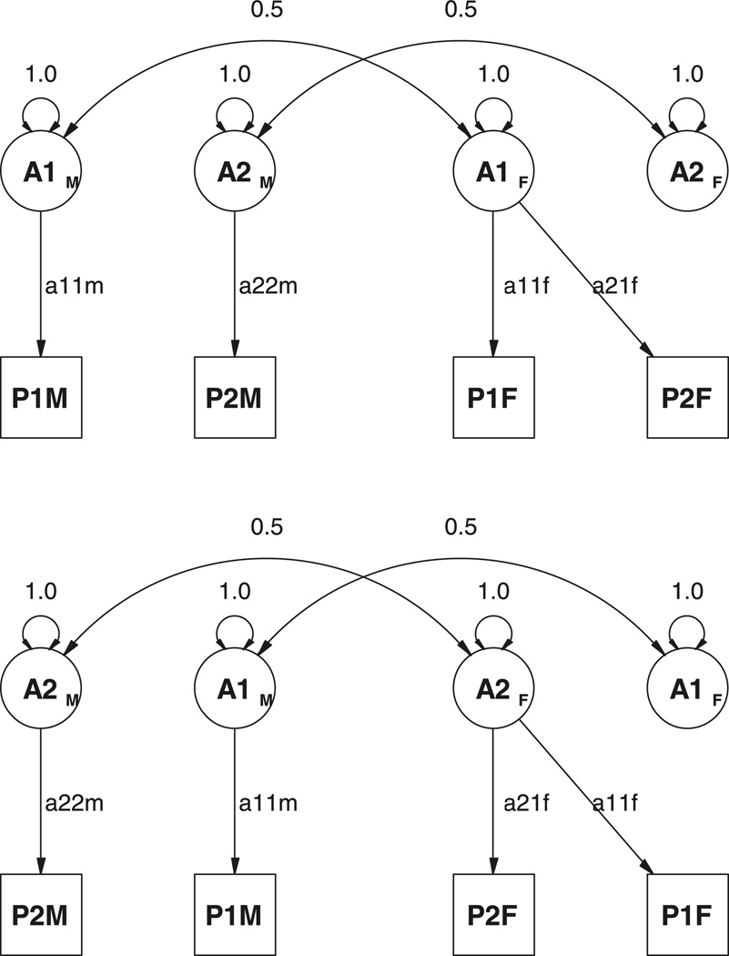
where I is the identity matrix. This result reflects what can be found by inspection of the path diagrams in Figure 4, namely that the first variable in males can correlate with both variables in the female, but the second variable is independent of them. The independence of the second variable is maintained regardless of the order of the variables in the data analysis. It is unlikely that a model which specifies that, for example, height in males is uncorrelated with weight in females would fit exactly the same as one that specifies that weight in males is uncorrelated with height in females. Thus the order of the variables in the analysis affects the ability of the model to account for the opposite-sex data. This is a very undesirable property of this model, which stems from misspecification of the original concept, that the same factors influence males and females, but that they do so to a different degree.

Figure 3.

Path diagrams for hypothetical results of model fitting of two phenotypes in two models of sex limitation to data from twins. Top: DZ male twins; bottom: DZ female twins.

Figure 4.

Path diagrams for hypothetical results of model fitting of two phenotypes in two models of sex limitation to data from twins. Top: DZ opposite-sex twins with variable 1 first; bottom: DZ opposite-sex twins with variable 2 first.

A further issue with the Cholesky decomposition has been described by Carey (2005). In brief, this issue stems from restricting the covariance matrices to be nonnegative definite. The distribution of the fit statistic used to assess overall model fit does not follow the χ² distribution.

Method

We consider two methods to solve the problem. First is the explicit specification of the model in terms of equal correlation matrices. Second is the application of non-linear constraints to the Cholesky decomposition to impose an equal correlation structure. We consider the utility of these models for specifying saturated models for the scalar and for the nonscalar sex limitation cases.

Scalar Sex Limitation

Correlation Approach

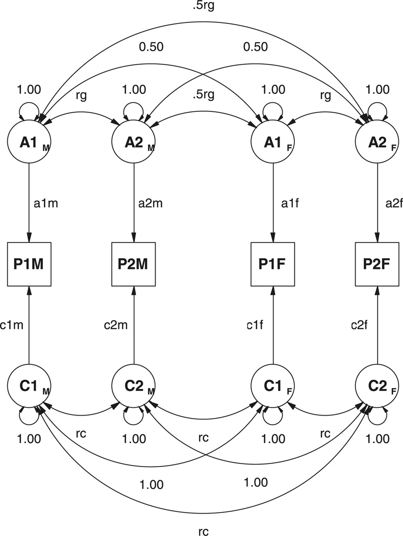
A correlational approach to the multivariate sex-limitation model is shown in Figure 5, for a pair of opposite-sex DZ twins. Note that the correlation between the additive genetic factors across the twins is set to equal .5r_g where r_g is the correlation between the additive genetic factors for the two phenotypes within an individual.

Figure 5.

Path diagram for a model of sex limitation in a pair of DZ opposite-sex twins using a correlation approach. Only the phenotypes P1_s, additive genetic factors, A1_s, and common environment factors, C1_s, are shown, in which 1 refers to trait 1 and subscript s refers to the sex of the twin.

The multivariate generalization of this model follows from considering the covariance matrix of A1_M, A2_M, A1_F and A2_F:

$$\begin{array}{c}A{1}_M\hfill \\ A{2}_M\hfill \\ A{1}_F\hfill \\ A{2}_M\hfill \end{array}\left[\begin{array}{cccc}A{1}_M\hfill & A{2}_M\hfill & A{1}_F\hfill & A{2}_F\hfill \\ \mathit{1}\hfill & r_g\hfill & .5\hfill & .5r_g\hfill \\ r_g\hfill & 1\hfill & .5r_g\hfill & .5\hfill \\ .5\hfill & .5r_g\hfill & 1\hfill & r_g\hfill \\ .5r_g\hfill & .5\hfill & r_g\hfill & 1\hfill \end{array}\right]$$

which can be written as a partitioned matrix:

$$\mathrm{G}=\left[\begin{array}{cc}\hfill {\mathbf{R}}_{\mathbf{G}}\hfill & \hfill .5\otimes {\mathbf{R}}_{\mathbf{G}}\hfill \\ \hfill .5\otimes {\mathbf{R}}_{\mathbf{G}}\hfill & \hfill {\mathbf{R}}_{\mathbf{G}}\hfill \end{array}\right]$$

Scalar sex limitation of these factors may be modeled through the diagonal factor loading matrices f = [a1_f a2_f] and m = [a1_m a2_m]. The predicted genetic covariance for opposite sex DZ pairs is given by:

$$[\begin{array}{cc}\hfill \mathbf{m}\hfill & \hfill \mathbf{f}\hfill \end{array}]\mathbf{G}[\begin{array}{cc}\hfill \mathbf{m}\hfill & \hfill \mathbf{f}\hfill \end{array}]\prime$$

It is immediately obvious that this revised model specification cannot generate the radically different covariance matrices for males (XX′) and females (YY′) in the Cholesky example. This new specification may generate different genetic covariance matrices for males and females, but it cannot generate different genetic correlation matrices. Therefore, the revised model will not always fit as well as the Cholesky model, but it is to be preferred because it is mathematically consistent with the scalar sex-limitation hypothesis.

A technical problem that remains with this approach is that it may still be desirable¹ to constrain the correlation matrix R_G to be positive definite. This constraint could be imposed by specifying the genetic correlation matrix as a (sex-invariant) triangular decomposition, and adding nonlinear constraints that force the diagonal elements to be equal to unity. However, the specification of additional parameters that this would require would increase computation time for parameter estimation. An alternative would be to add nonlinear inequality constraints on the eigenvalues of the matrix R such that they are all greater than or equal to zero. Either approach may be implemented in Mx.

Cholesky Decomposition Approach

The Cholesky decomposition has the advantage that it automatically generates positive semi-definite covariance matrices. That is, the correlations among the genetic factors and among the environmental factors are all bounded to lie in the closed interval −1 ≤ r ≤ 1, and do not violate reasonable ranges when considered in combination. It is also easy to specify in Mx and other programs that allow matrices to be declared as lower-triangular. The main problem is that it does not force the correlations between the factors to be equal for males and females. However, this constraint is quite easy to impose using Mx. To do so it is necessary to constrain the genetic and environmental correlation matrices to be equal. In order to constrain the predicted phenotypic covariance matrices of twins to be strictly positive definite, the diagonal elements of the specific environment Cholesky factor matrix should be constrained to be greater than zero.

To summarize, scalar sex limitation may be handled effectively with either the correlational approach or the modified Cholesky approach that constrains the genetic correlation matrices of males and females to be equal. Equivalently, this model may be thought of as specifying different sensitivity of each phenotype to its sources of variance. This differential response of the phenotype is forced to be the same for all sources of genetic variance — be they shared with other variables or specific to the phenotype itself. A further reduction of the model would be to specify that all sources of variance for a trait — genetic or environmental — are modulated equally by sex. We refer to this model as phenotypic scalar sex limitation. It is an empirical question whether this model would provide a more parsimonious explanation of the data.

Nonscalar Sex Limitation

Correlational Model

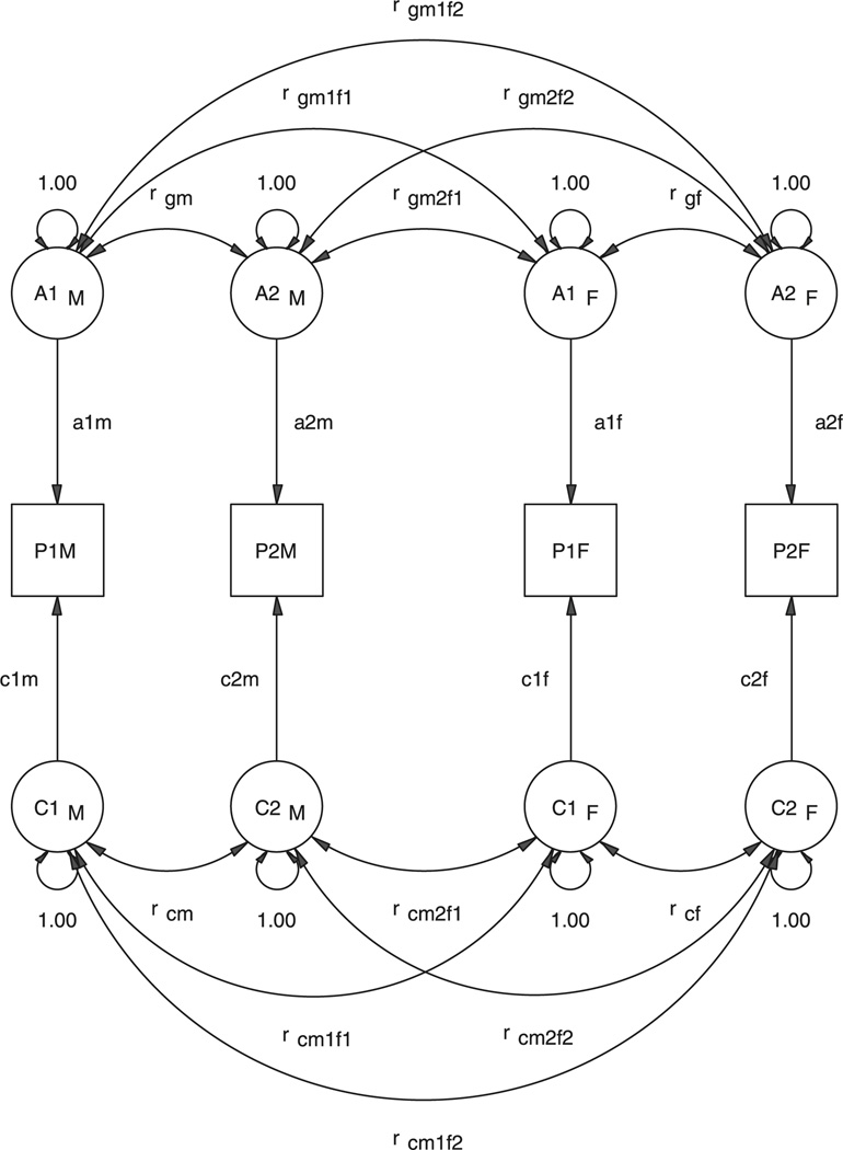
One simple approach to nonscalar sex limitation is to modify the correlational model. This modification is shown for the bivariate case in Figure 6. In this model, all six of the correlation paths for the genetic factors are allowed to be estimated as separate free parameters, and that the same is true of the common environment factors. Certain restrictions on these parameters would reduce the model to one of scalar sex limitation, per Figure 5.

Figure 6.

Path diagram for a model of sex limitation in a pair of DZ opposite-sex twins using a correlation approach. Only the phenotypes P1_s, additive genetic factors, A1_s, and common environment factors, C1_s, are shown, in which 1 refers to trait 1 and subscript s refers to the sex of the twin.

The .5r_g may be replaced by .5r_gmf.r_g where r_gmf denotes the genetic correlation across males and females for this pair of traits. If the same genetic factors influence both males and females, the correlation r_gmf = 1 (scalar sex limitation); if they are entirely different (independent), r_gmf = 0 (complete nonscalar sex limitation); and otherwise 0 < r_gmf < 1 (incomplete nonscalar sex limitation).

Each latent factor for males correlates .5 with its counterpart in females when sex limitation is scalar. In fact, the within-person genetic matrix as a whole is multiplied (Kronecker product) by the scalar .5 to obtain the m × m block of genetic correlations between opposite-sex twin pairs. In the event that the factor structure differs between males and females, three separate matrices of correlations may be estimated. One, the correlations between factors in males, two, the correlations between factors in females, and three the correlations between male and female factors. All three matrices are of order m × m but only the correlations across males and females may be asymmetric. This model is saturated, but is not guaranteed to be positive definite. Nonlinear constraints on the eigenvalues of the genetic correlation matrix should be imposed.

Cholesky Model

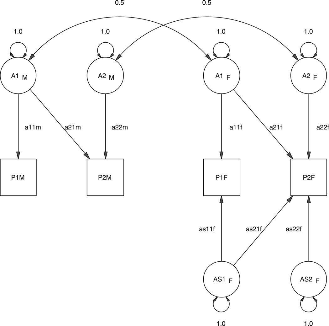
The constrained Cholesky model for scalar sex limitation may also be revised to allow for nonscalar sex limitation. Suppose we permit three sets of factors: F_CM, which affect males and have the same correlation structure as F_CF which affect females, and F_SF which are specific to females and do not affect males. In the event that the data are completely consistent with a model of scalar sex limitation, the parameter estimates of F_SF would be estimated to be zero. A diagram of this model is shown in Figure 7 for the bivariate case. The paths a_ijm, a_ijf and as_ijf would be elements of the matrices F_CM,F_CF and F_SF, respectively. Should the influences be completely different in males and females, that is, all the opposite-sex correlations are zero, the estimates of the scalar factor loadings F_CF would be estimated to be zero. The positive semi-definite constraint is automatically maintained by the Cholesky decomposition (Appendix A Theorem 3). Also, the constraint on the scalar part of the model, that the factor correlations should be equal, is retained from the scalar case.

Figure 7.

Path diagram for a model of nonscalar sex limitation in a pair of DZ opposite-sex twins using a correlation approach. Only the phenotypes P1_s and additive genetic factors, A1_s, are shown, in which 1 refers to trait 1 and subscript s refers to the sex of the twin

Maintaining this constraint lends the model the positive feature that it is invariant to the ordering of the variables. However, this model is problematic, in that it will not fit certain datasets as well as the correlational model. It uses fewer parameters and will fail to account for certain patterns of correlation. That is, it is not suitable as a ‘saturated’ model. Since a saturated genetic covariance structure is a primary goal of the approach, it must be concluded that this model is less useful than its correlational counterpart.

Comparison of Implementations

Of these two implementations of nonscalar sex-limited effects, the correlational and the Cholesky, only the former fully saturates the predicted covariances between opposite-sex twins. When m variables are measured from opposite-sex pairs, there are m² observed cross-sex covariances. In practice, this block of covariances need not be symmetric. For example, the correlation between height in females and height in their male co-twins may not be the same as the correlation between weight in females and height in their male co-twins. The nonscalar sex-limitation models considered thus far require m² parameters in the correlation model, and m(m + 1)/2 parameters in the Cholesky model to account for possible reductions in resemblance between opposite-sex twin pairs. Therefore, the correlational model will fit at least as well as the Cholesky model, albeit at the expense of more parameters.

The conceptual basis of the correlational model is not without its problems. Different across-sex genetic correlations may be observed but their interpretation becomes more difficult. The division into general factors that affect both sexes and factors that are specific to only one sex is no longer retained. The correlational model becomes more of a description of the observed data rather than a model for the origin of gender differences. Nevertheless, it is possible to specify the across-sex correlations as a symmetric matrix to test hypotheses concerning whether, for example, the genetic correlation between height in females and weight in males is the same as that between weight in females and height in males.

Discussion

Two approaches to the treatment of scalar sex limitation have been considered. One is to specify the model in terms of factors for males and females and to estimate correlations within male factors, and within female factors. These factors are constrained to have the same correlation matrix in males and females. The factors then influence the phenotype via path coefficients which are not constrained to be equal across sexes. Thus the model specifies that the same factors influence males and females but that they may do so to different degrees. The second, equivalent approach specifies a Cholesky model for factors that differ between the sexes only in the scale of their effects, not in their correlations. Ordinarily, the Cholesky factor model does not preserve the equal-correlation constraint, but this can be imposed by a series of nonlinear equality constraints that equate the genetic or environmental correlations in males with their counterparts in females. This Cholesky model has the advantage that the A, C and E covariance matrices are constrained to be nonnegative definite, and it is simple to ensure that the E covariance matrix is strictly positive definite, thereby ensuring positive definiteness of the predicted covariance matrix between twins (Appendix A, Theorem 3).

Nonscalar sex differences occur when different factors influence variation in the two sexes. To model differences of this sort is a more challenging task. One approach is to take the correlational model for scalar sex limitation, to remove the restriction that the correlation matrices are equal for males and females, and then to estimate all of the m × m cross-sex correlations. In the classical twin study it is necessary to estimate only one of these cross-sex correlation matrices, either the additive genetic or the common environment, or the dominance genetic, because MZ opposite-sex pairs do not exist. The correlational model is a saturated model, in that all of the cross-sex covariances have a corresponding cross-sex parameter to be estimated. However, certain constraints may reasonably be imposed on these cross-sex covariances. For genetic cross-sex covariances in DZ twins or siblings, it would be natural to constrain them to lie between −.5 and .5, which corresponds to the reasonable range of −1 to 1 for within-person genetic correlations. Similarly, it would be reasonable to expect common environment correlations to lie between −1 and 1. Furthermore, the overall common environment or genetic covariance matrices for pairs of twins should be nonnegative definite. Therefore, it may be desirable to impose a series of nonlinear constraints on the correlational model to ensure that these restrictions are met. We also note that even if a fully saturated correlational model for sex limitation is fitted, it may not describe the data perfectly. For example, suppose that the set of variables under analysis comprises two subsets, one where familial resemblance is due to A, while the other is due to C. Specifying only genetic or only common environment correlations would assist in the prediction of across-sex covariance of only one of the two subsets. In this case, it would be possible to specify a multivariate model that contains a different form of sex limitation for different subsets of variables, although the investigator should be careful not to capitalize on chance by first inspecting the data and results and then specifying the sex-limitation model accordingly.

An alternative but more restricted form of sex-limitation model may be specified by adding a component to the Cholesky factorization. The modified sex-limited Cholesky factor model with equated correlations for males and females is augmented by a component specific to either males or females only. This model involves fewer additional parameters than the non-scalar correlational approach; whether it provides a more parsimonious fit to the data than the correlational model will depend on the dataset being analyzed. It is also worth noting that the same fit may not be achieved if the additional factor matrix is added to the males or the females.

The Cholesky decomposition was originally intended for use as a robust way to estimate genetic (or other variance-component) covariance matrices while constraining them to be nonnegative definite. In the single-sex case, it is a saturated model for these covariances, because it has as many parameters as there are available statistics. Its fit provides a yardstick for goodness-of-fit against which other multivariate models may be compared — albeit with caveats (Carey, 2005). Two main varieties of multivariate model are widely used in genetic epidemiology. The ‘independent pathway’ or ‘biometric factor’ model (Kendler et al., 1987; McArdle & Goldsmith, 1990; Neale & Cardon, 1992) specifies general genetic and environmental factors that may have direct effects on all the observed phenotypes. The ‘common pathway’ or ‘psychometric factor’ model involves an intermediate latent factor between the genetic and environmental general factors and the observed phenotypes. Under certain conditions, these alternative models may also suffer from the problems with the use of the Cholesky decomposition in models for sex limitation. The psychometric model specifies a single latent variable which influences a number of traits. This latent variable is usually specified to have genetic and environmental factors. As such, the model is directly derived from the single factor model commonly used for the analysis of data from unrelated individuals. An extension of this model is to specify two or more such latent variables, which may be independent (i.e., orthogonal) from each other, or correlated (i.e., oblique). In the oblique case, it is possible to decompose the covariation between latent factors into genetic and environmetal components. To account for data collected from same-sex and opposite-sex relatives, this model faces the same difficulties as those of the scalar and non-scalar sex-limitation models described in this article. Essentially, the sex-limitation specification problems arise at the level of the genetic correlations between factors, instead of at the level of the genetic correlations between observed variables. The problems, and the solutions suggested in this article, apply equally to multivariate genetic and environmental covariance structures regardless of the level at which they are found in a model.

One further point to note is that it is possible to perform a limited version of a test for nonscalar sex limitation with same-sex twin pairs alone. If the genetic correlation between two traits is found to differ between male-male and female-female pairs, then there is evidence that there are some factors that operate in only one of the sexes. Using same-sex pairs alone, there is no way to determine directly which of the two variables has nonscalar sex limitation, but it can be useful to establish that at least one of the traits has this characteristic. Some triangulation as to which has and which does not could be achieved in the multivariate case. Suppose that only one trait, x, in a set A had nonscalar genetic sex limitation. One could expect to find evidence of sex differences in genetic correlations in bivariate analyses of trait x with every other trait in the set. Conversely, analyses of pairs of traits that exclude trait x would not show evidence of a female-male difference in genetic correlation. The real world may prove more complex than this simple example, but it is still interesting that studies of datasets that do not contain opposite-sex pairs can, in principle, provide information about nonscalar sex limitation.

Finally, we note that constraining covariance matrices to be nonnegative definite may not always be desirable. Carey (2005) discusses the complex distributional properties of the test statistics when such constraints are employed. Most salient in the present context is the question of whether or not a variance component could generate nonnegative definite covariance structures. In principle, any process that generates a quantitative phenotypic difference (such as when different mean values are observed for different genotypes at a diallelic locus) must generate a positive amount of variance in that trait. If it affects two traits, it cannot cause their covariance to be greater than the root of the product the variance that it causes in each. That is, it cannot make them correlate greater than 1.0 or less than minus one. Should we observe that unrestricted estimates of genetic covariance matrices are negative definite more often than we would expect by chance, it would likely imply that the model is incorrect. In the univariate classical twin study, if the additive genetic, shared and specific environment (ACE) model was the only model fitted, and if population variance was entirely due to additive genetic and specific environment factors (AE), then half the time we would expect to see a negative estimate of the shared environment variance. If population variation was also due to non-additive genetic factors (e.g., under an ADE model), then asymptotically the estimate of C would always be negative. Given a sufficiently large sample size, we would observe significantly negative estimates of C, which is the simplest example of a negative definite covariance matrix. Therefore, it seems prudent to compare the fit of an unrestricted model — without component matrices constrained to nonnegative definite — to that of the model that imposes this constraint, in order to provide a further test of the suitability of the model for explaining trait variation and covariation in the population under study.

Appendix A

Notes on Matrix Algebra

Similar results may be found in Searle (1992).

Theorem 1 Matrices generated from a Cholesky or Triangular decomposition C = LL′ are positive semi-definite.

Proof: The definition of positive semi-definite is that the product x′Cx ≥ 0 for all nonnull vectors x. In the present case we can substitute LL′ for C and obtain

$$\mathbf{x}\prime \mathbf{L}\mathbf{L}\prime \mathbf{x}=(\mathbf{x}\prime \mathbf{L})(\mathbf{x}\prime \mathbf{L})\prime$$

The term on the right is the inner product of the vector x′L and is therefore a sum of squared real numbers, which has a lower bound of zero.

Theorem 2 Matrices generated from a modified Cholesky decomposition C = JJ′, where the diagonal elements of J are constrained to be strictly positive, are positive definite.

Proof: From the proof of Theorem 1, we have

$$\mathbf{x}\prime \mathbf{J}\mathbf{J}\prime \mathbf{x}=(\mathbf{x}\prime \mathbf{J})(\mathbf{x}\prime \mathbf{J})\prime$$

in which the minimum of any term of the right hand side is zero. Let the dimension of J be n. If the last element of x (i.e., x_n) is not equal to zero, then the i^th element of x′J will equal $x_i^{\mathit{2}}{J}_{ii}^{\mathit{2}}$ which will be greater than zero since the element J_nn is constrained to be greater than zero. If element x_n is zero, then element n − 1 of x′J would take its minimum value of zero if and only if x_n−1 is zero. By induction, therefore, the product x′(JJ′)x would be zero only if all elements of x are zero, which is the null vector excluded from the definition of positive definiteness.

Theorem 3 Any matrix formed by the sum of a set of positive (semi-)definite matrices is positive (semi-)definite.

Proof: This follows directly from the observation that matrix multiplication is distributive over addition, i.e., A(B + C) = AB + AC. For positive definiteness, since x′ (A + B)x = x′Ax + x′Bx and by definition x′Ax > 0 and x′Bx > 0, the sum x′Ax + x′Bx must be greater than zero, as must x′(A + B)x. For positive semi-definiteness, the > can be replaced by ≥.

References

- Carey G. Cholesky problems. Behavior Genetics. 2005;35:653–665. doi: 10.1007/s10519-005-5355-9. [DOI] [PubMed] [Google Scholar]
- Eaves LJ, Last K, Young PA, Martin NG. Model fitting approaches to the analysis of human behavior. Heredity. 41:249–320. doi: 10.1038/hdy.1978.101. (978). [DOI] [PubMed] [Google Scholar]
- Kendler KS, Heath AC, Martin NG, Eaves LJ. Symptoms of anxiety and symptoms of depression: Same genes, different environments? Archives General Psychiatry. 1987;44:451–457. doi: 10.1001/archpsyc.1987.01800170073010. [DOI] [PubMed] [Google Scholar]
- Lubke GH, Dolan CV, Neale MC. Implications of absence of measurement invariance for detecting sex limitation and genotype by environment interaction. Twin Research. 2004;7:292–298. doi: 10.1375/136905204774200578. [DOI] [PubMed] [Google Scholar]
- Maes HH, Neale MC, Martin NG, Heath AC, Eaves L. Religious attendance and the frequency of alcohol use: Same genes or same environments: A bivariate extended twin kinship model. Twin Research. 1999;2:169–179. doi: 10.1375/136905299320566031. [DOI] [PubMed] [Google Scholar]
- Martin NG, Eaves LJ. The genetical analysis of covariance structure. Heredity. 1977;38:79–95. doi: 10.1038/hdy.1977.9. [DOI] [PubMed] [Google Scholar]
- Mather K, Jinks JL. Introduction to biometrical genetics. Ithaca, New York: Cornell University Press; 1977. [Google Scholar]
- McArdle JJ, Goldsmith HH. Alternative common-factor models for multivariate biometric analyses. Behavior Genetics. 1990;20:569–608. doi: 10.1007/BF01065873. [DOI] [PubMed] [Google Scholar]
- Meredith W. Measurement invariance, factor analysis, and factorial invariance. Psychometrika. 1993;58:525–543. [Google Scholar]
- Neale MC, Cardon LR. Methodology for genetic studies of twins and families. Dordrecht: Kluwer Academic Press; 1992. [Google Scholar]
- Neale MC, Walters EE, Eaves LJ, Maes HM, Kendler KS. Multivariate genetic analysis of twin-parent data on fears: Mx models. Behavior Genetics. 1994;24:119–139. doi: 10.1007/BF01067816. [DOI] [PubMed] [Google Scholar]
- Searle SR. Matrix algebra useful for statistics. New York: John Wiley; 1992. [Google Scholar]
- Vandenberg SG. Multivariate analysis of twin differences. In: Vandenberg SG, editor. Methods and goals in human behavior genetics. New York: Academic Press; 1965. pp. 29–43. [Google Scholar]