

Abstract
• Background and Aims The morphogenesis and architecture of a rice plant, Oryza sativa, are critical factors in the yield equation, but they are not well studied because of the lack of appropriate tools for 3D measurement. The architecture of rice plants is characterized by a large number of tillers and leaves. The aims of this study were to specify rice plant architecture and to find appropriate functions to represent the 3D growth across all growth stages.
• Methods A japonica type rice, ‘Namaga’, was grown in pots under outdoor conditions. A 3D digitizer was used to measure the rice plant structure at intervals from the young seedling stage to maturity. The L-system formalism was applied to create ‘3D virtual rice’ plants, incorporating models of phenological development and leaf emergence period as a function of temperature and photoperiod, which were used to determine the timing of tiller emergence.
• Key Results The relationships between the nodal positions and leaf lengths, leaf angles and tiller angles were analysed and used to determine growth functions for the models. The ‘3D virtual rice’ reproduces the structural development of isolated plants and provides a good estimation of the tillering process, and of the accumulation of leaves.
• Conclusions The results indicated that the ‘3D virtual rice’ has a possibility to demonstrate the differences in the structure and development between cultivars and under different environmental conditions. Future work, necessary to reflect both cultivar and environmental effects on the model performance, and to link with physiological models, is proposed in the discussion.
Keywords: Rice, Oryza sativa, morphogenesis, plant architecture, L-system, 3D modelling
INTRODUCTION
A significant part of the success of the ‘Green Revolution’ in the 1960s resulted from the breeding of grain crops that had a more efficient plant architecture (Khush, 1996). The modern varieties were markedly shorter through allocation of a greater proportion of resources to grain production at the expense of vegetative growth. High-yielding varieties of rice, Oryza sativa, have doubled the annual yield per unit area obtained in some countries (Conway, 1997). Even so, there is concern that over the same period, and in the context of continued increase in demand, the yield potential has not increased and some fundamental limit might have been reached (Khush, 1996; Conway, 1997).
Considerable activity is underway to investigate whether the suspected limit can be extended by changes in fertilizer application rates and timing (Dobermann et al., 2000), by increasing nutrient-use efficiency (Cassman et al., 1998; Fischer, 1998; Ladha et al., 1998; Sheehy et al., 1998), by breeding new plant types for rice (Peng et al., 1994; Khush, 1996; Khush and Virk, 2002) and by use of hybrid rice (Khush, 1996; Khush and Virk, 2002). An excellent start to structuring an integrated body of information for ecophysiological factors affecting yield has been made in the form of ‘rice crop’ models (Ritchie et al., 1987; Horie, 1987; Penning de Vries et al., 1989; Graf et al., 1990; Kropff et al., 1994; Hasegawa and Horie, 1997; Wu and Wilson, 1998). The major components still required for a broader investigation are numerical specifications of morphogenesis, interactions between physiology and morphogenesis, and effects of the resulting plant architectures on resource acquisition. This paper takes a small step towards filling these gaps by presenting a numerical specification and simulation model of morphogenesis in rice.
The geometrical structure of a rice canopy has been investigated for optimization of light penetration, photosynthesis activity and yield in relation to breeding programs (Tsunoda, 1959; Tanaka et al., 1969). Simple methods to measure leaf geometry have been developed (Ito, 1969), and canopy structure differences between some cultivars have been investigated (Ito et al., 1973). These data were used to study the radiation environment and photosynthesis in the canopy (Udagawa et al., 1974a, b). The canopy structure, leaf area distribution and nitrogen distribution have been introduced in some simulation models (e.g. Kropff et al., 1994; Hasegawa and Horie, 1997). The dynamic aspect of canopy structure development, however, has not been modelled to allow for the differences of plant architecture between cultivars and its effects on growth and yield. Now, the necessary tools for obtaining and manipulating information on plant architecture are available for some plant species, including cereals (e.g. Sinoquet et al., 1991; Boissard et al., 1996; Room et al., 1996; Sinoquet et al., 1998; Takenaka et al., 1998; Kaitaniemi et al., 1999; Shibayama, 2001), and new approaches to the design of plants are starting to be investigated (Mabrouk et al., 1997; Sinoquet et al., 1998). This paper reflects current renewed recognition of the fundamental importance of plant architecture and morphogenesis (Sattler and Rutishauser, 1997), which is being explored in an increasing range of crops (de Reffye et al., 1995; Fournier and Andrieu, 1998; Perttunen et al., 1998; Kaitaniemi et al., 2000). Rice plants follow general features of plant architecture development and morphogenesis, but produce a substantial number of tillers and leaves compared to other major cereals and dicotyledonous species. While these are the key yield determinants of this species, a 3D-architecture model of a plant with many cohorts has been difficult to develop. In fact, previous 3D cereal crop models (e.g. Fournier and Andrieu, 1998 for maize, and Kaitaniemi et al., 2000 for sorghum) do not include tillering (branching) processes. The present study, therefore, is an attempt to reproduce dynamics of a 3D-architecture of an isolated rice plant including leaf and tiller number modules. Canopy architecture development can be influenced by resource competition and micro-climatic conditions, but here we propose an isolated plant version of 3D rice as the prototype to be used for future canopy versions of the model.
First the morphogenesis and development of rice plant architecture is described based on our experimental measurements using a 3D sonic digitizer, using methods similar to Sinoquet et al. (1991) and Kaitaniemi et al. (1999). Then a 3D structural model ‘virtual rice’ is constructed based on the L-system formalism (Lindenmayer, 1968). Production rules of organs are described using L-system syntax according to the rice growth pattern, and empirical functions for the development of plant parts and phenological models are incorporated into the 3D structural model.
MATERIALS AND METHODS
Growing conditions
Plants of the japonica-type rice Oryza sativa L. ‘Namaga’ were grown in the open at the CSIRO Long Pocket Laboratories, Brisbane, Australia (27°28′S, 153°02′E) between September 1997 and February 1998. After germination, two seeds were sown per 25 cm2 in a seedbed filled with loamy soil and fertilizer (N : P : K = 5 : 5·5 : 4 gm−2). At the 3rd leaf stage, 16 d after appearance of the first leaf, one of each pair of plants was removed to leave a stand of uniform plants. Seedlings were transplanted singly into 17·5-cm diameter pots filled with the same soil and fertilizer (N : P : K = 10 : 11 : 8 gm−2 ). The pots were placed next to each other so that plants were about 18 cm apart. Urea was applied twice during growth before panicle initiation (5 g N m−2), and again at 10 g N m−2 after panicle initiation but before flowering. An automatic weather station recorded daily maximum and minimum temperatures, which were used to calculate cumulative degree-days above a base of 10 °C (d10; Gao et al., 1987) from the appearance of the first leaf above the soil surface, thus:
 |
Measurement of architectural development
Every day, records were made of the new leaves and tillers that emerged. A new leaf was considered to have emerged when its tip appeared above the preceding leaf sheath, and each new leaf was marked with its sequence number in black ink. The 3D geometry of all plants was measured using a GTCO Freepoint 3D sonic digitizer interfaced to special software (FLORADIG©). The system was the same as in the report of Kaitaniemi et al. (1999). The software records 3D co-ordinates labelled according to the types and topological positions of plant parts (Hanan and Room, 1997). Between four and six plants were measured at 16, 30, 37, 43, 54, 58, 72 and 97 d after appearance of the first leaf.
The rice plants were brought inside to the laboratory for digitizing to avoid disturbance by wind. Prior to plant measurements, the accuracy of the digitizer was checked with the ruler; five 10-cm segments were measured at various positions and angles in space. If the digitized length ranged within 2 mm, digitization of the rice plants was undertaken. If not, the digitizer and conditions were checked before plants were measured. Before digitizing a plant, reference axes were set, with two points on a weighted string and two painted marks on the pot rim acting as vertical and horizontal references, respectively.
In order to describe curved leaf blade lengths accurately with digitization, a preliminary set of measurements was done. Two, three and five points along the midrib were used to digitize leaf blade lengths that varied between 50–350 mm, and these data were compared using regression analysis with lengths measured by a ruler. The regression coefficients between the real length as measured by the ruler (y) and the digitized length (x) were 1·259, 0·966 and 0·990 for two, three and five points respectively. Therefore, we usually digitized three points, the collar, mid-point and tip of each leaf. In addition, nine-point digitizing was carried out on leaves in various positions on the main stem and tillers in order to find the mathematical function of the axial curves of leaf blades.
The maximum width of the blade was measured for leaves in various positions on the main stem and on tillers using a ruler, since the leaf blade width was too narrow to measure with the digitizer.
Leaf positions were numbered from ‘1’ at the basal node of the main stem or a tiller. Primary and secondary tillers are those that emerged from the main stem and primary tillers, respectively. Measurements were non-destructive, so that ‘sheath length’ refers to the section of sheath visible between the collar of a leaf and the base point of the stem or tiller, using two points. The panicle was digitized at the neck node and the panicle tip.
To describe the outline shape of blades, the width of the blade was measured at different positions using a ruler. A different set of rice plants was used for this as it involved destructive measurements, since accurate measurements on intact plants were difficult. Because the internodes were not visible, destructive sampling was also used to measure them (using a ruler) after final digitizing of mature plants.
Data processing and analysis
The 3D co-ordinates collected were processed by the software VPCONV© to calculate lengths and orientations, which were labelled and stored in comma-delimited files. The latter files were imported into a Microsoft Access© database together with records of thermal time expressed as d10 from seedling emergence. Standard database query procedures were used to select subsets of data for analysis. Linear and non-linear regressions were applied to determine the parameters of the functions that describe both growth and structure of the rice plants. CurveExpert 1·3 (Hyams, 1997) was used for these statistical analyses.
Modelling
The results of statistical analyses were expressed as specifications, or rules, of morphogenesis using the L-system formalism (Lindenmayer, 1968; Prusinkiewicz and Hanan, 1989; Prusinkiewicz and Lindenmayer, 1990). In this formalism, the architecture of a plant at any time is represented by a string of characters and associated parameters. Different characters symbolise different organs, topology is represented by the relative positions of the characters in a string, and parameters keep track of individual organ characteristics such as age, length, width and colour of each organ. ‘Production rules’ of the form
 |
specify that the predecessor, representing current plant parts, gives rise to the successor, representing new ones and how parts change in size, shape and other characteristics, in each time step that the condition is true. In this work, a time step of one day was used.
Development stage
The developmental index (DVI, DV) (Nakagawa and Horie, 1995) was applied to represent the physiological development of the rice plant. The DVI is a continuous variable and defined as 0 at first leaf emergence, 1·0 at panicle initiation, 2·0 at heading and 3·0 at maturity. Observations were made of first leaf emergence, heading and maturity of digitized plants, and panicle initiation was checked by dissection using a different set of plants for destructive sampling.
The DV is an accumulation of developmental rate (DVR, DR), which is a function of daily mean temperature (T) and photoperiod (L):
 |
where DR,i is the developmental rate for the ith day from the start, calculated according to Nakagawa and Horie (1995) and Hasegawa et al. (1995), as functions (f and g) as follows.
When DV < 1·0:
 |
When 1·0 ≤ DV < 2·0
 |
When 2·0 ≤ DV ≤ 3·0
 |
 |
 |
where Gj is the minimum number of days required for completing each phase, vegetative (j = 1) and reproductive (j = 2), and DV*j marks the start (j = 1) and end (j = 2) of the photosensitive phase. aj, Thj, Tc, bj and Lc are parameters for determining the shape of the functions.
Leaf number
Phyllochron, or Haun stage, of the plant is often expressed as a function of temperature (e.g. Miglietta, 1991; Yin and Kropff, 1996) but daylength is also known to influence the final leaf number (Nakagawa and Horie, 1991). According to H. Nakagawa et al. (unpubl. res.), the leaf number, LN, and leaf emergence rate, LR, are expressed as follows.
For 0 < DV < 1
 |
For 1 ≤ DV < 2
 |
where GL, AL, TL, CL, DL and EL are parameters, T is daily mean temperature, DV is calculated by eqn (2) and LN0 is the initial leaf number at transplanting, in this case 1.
Since there were no pre-existing parameters for phenological development of ‘Namaga’, we applied the parameter set of ‘Koshihikari’ for the DVI calculation, and that of ‘Nipponbare’ for the leaf development. The development parameters of these cultivars were obtained from Nakagawa and Horie (1991, 1995).
Vegetative development
During vegetative development in all grasses, including rice, each apical meristem produces a module that consists of a series of metamers (Room et al., 1994). Each metamer is comprised of an internode with, at the distal end, an axillary meristem and a leaf sheath connected to a leaf blade. Some axillary meristems remain dormant while others, through growth, become the apical meristems of branches and give rise to vegetative tillers. Vegetative development was expressed as a parametric L-system production of the form:
 |
where A is an apical meristem, I is an internode, B is an axillary bud, S is a leaf sheath and L is a leaf blade. Each component has parameters level, i, j, k, l, tsum, and DV. Level is the rank of a parent branch, from 0 for the main stem, 1 for a primary tiller, 2 for a secondary tiller and so on. The parameters i, j, k and l indicate node of attachment to the main stem, primary tiller, secondary tiller and tertiary tiller, respectively. Fourth or higher order tillers rarely emerge in practice, therefore we did not take higher orders into account in the current model. The daily increment in heat units, t(d10), experienced by an organ, is accumulated as:
 |
where ‘day’ is the number of days after appearance of the organ, with tsum0 = 0 at the time of appearance. The parameter DV is a DVI at the leaf appearance. For example, A(0,5,0,0,0,80,DV) is the apex on the 5th node of main stem, of which the leaf appeared at a DVI of DV with an accumulated heat unit of 80. Likewise, A(1,3,2,0,0,…) is the apex on the 2nd node of the 3rd primary tiller. If the primary tiller produces a secondary tiller, eqn (10) is expressed as
 |
In rice, a new module or tiller has the potential to emerge from the axil of every leaf. An axillary bud at the nth node of its parent module produces the first leaf of a daughter tiller at the same time as the leaf emerges at node n + 3 on the parent module (Katayama, 1951). This is represented by:
 |
where ‘condition’ is that the parent module has just initiated a leaf on the node 3 position distal to the axillary bud in question.
The axial angle between a parent module and its daughter tiller increases with the number of tillers produced by the parent module above and on the same side as the daughter tiller, and with the number of tillers produced by the daughter tiller. Context-sensitive L-system productions (Prusinkiewicz and Lindenmayer, 1990) were used to model this relationship (see Appendix). Increase of the axial angle stops when the plant goes into the reproductive stage. Internode elongation starts after the panicle initiation, DVI = 1·0.
Reproductive development
The onset of reproductive development occurs when the apical meristem, A, transforms into the last internode, In, and the panicle initial, P, at the time the developmental index, DVI, exceeds the panicle initiation threshold 1·0:
 |
Internode elongation starts with panicle initiation. The panicle develops in such a way that the necknode differentiates first followed by rachis branches and spikelets. Thus,
 |
 |
where p1 is the order of the rachis branch, p2 is the number of the branches on each parent branch, and G is the spikelet. p1 max and p2 max are the maximum values of p1 and p2, and Ip1,p2 is the rachis branch, which depend on the cultivar and the growth conditions.
Simulation
The L-system model was constructed and operated in the Virtual Laboratory in Botany (vlab) computing environment (Prusinkiewicz and Lindenmayer, 1990) running on a Silicon Graphics IRIX computer. L-system productions were interpreted by the Plant and Fractal Generator program (cpfg) (Mech, 1998; Prusinkiewicz et al., 2000). The L-system produces a string of symbols in each time-step, and then cpfg uses the ‘Homomorphism’ rules to translate the string into a visual form with 3D graphics. Parameters in each module, such as topological position and age, and external information, such as temperature, were used for the calculation of size and angle of each module.
RESULTS
Observations of morphogenesis
Leaf blade length. Fully expanded leaf blades were longest on the main stem and decreased in size on successive tillers (Fig. 1). The ‘positions’ of leaves on the primary tiller were transformed to the positions of leaves that emerged at the same time on the main stem by using the observation that a leaf at node ‘m’ of a tiller attached to parent module node ‘n’ always emerges at the same time as the leaf at parent module node n + m + 2 (Katayama, 1951). Thus, for example, the leaf attached to node 3 of the second primary tiller corresponds to the leaf attached to node 7(2 + 3 + 2) on the main stem. Accordingly, the position of any leaf, L(level, i, j, k, l), on the tiller can be translated to a comparable position of a leaf on the main stem (Relative Leaf Position, RLP, Goto, 2003) as follows:
 |
where i, j, k, l and level are the same parameter as in eqn (10).
Fig. 1.

The length of fully expanded leaf blades of rice on the main stem and the primary tillers. M, main stem; 2–6, 2nd to 6th primary tillers, with respect to the position of the main stem leaf that was produced at the same time. Vertical bars show standard errors. Lines show curves fitted with eqns (17)–(19).
The lengths of leaves on each RLP can be expressed by a family of curves having a truncated normal distribution:
 |
Where Ln is length of the leaf blade at position n, Lmax is the maximum length of any blade in the same module, nmax is the position of the longest blade in the module, and d is a parameter that adjusts the spread of the distribution. For the main stem, the values of these parameters were Lmax = 428 mm, nmax = 10·8, and d = 3·84.
Lmax and d for a primary tiller were functions of the position of attachment of the tiller to the main stem (Pt):
 |
 |
The value of nmax varied only from 10·8 to 11·4 between tillers and we used a constant value of 11 in the model. Goodness of fit between the measured leaf blade length and the simulated Ln was evaluated by the root-mean-squared error (RSME) and R2. The values of RSME were from 27·7 to 39·3 mm and R2 varied from 0·89 to 0·97 among the main stem and primary tillers. For the secondary tiller, since only a few data sets were available from the results, we employed the same relationship of Lmax and d as for the 6th primary tiller. No tertiary tillers were observed in the experiment.
Measurements were insufficiently frequent to allow precise estimates of how the rate of leaf elongation varied with time. Kawahara et al. (1968) and Arashi and Eguchi (1954) reported S-shaped growth curves of leaf blade length (Llen), but no specific formulae were given. We assumed a logistic pattern and fitted the following equation:
 |
where Lmax,n is the final leaf length for each leaf position calculated from eqns (17)–(19), tsum is cumulative d10 from the start of leaf emergence, and D is the duration in d10 from leaf emergence to complete expansion. Kawahara et al. (1968) reported that the duration of leaf expansion was prolonged after panicle initiation. We thus arbitrarily used D = 50 until DVI = 1·0, and D = 120 for after DVI = 1·0.
Leaf blade width. The maximum width of leaf blades had an overall asymptotic relationship to blade length, and results for main stem, tiller and flag leaves fell into distinct groups (Fig. 2). The same function was fitted to all three groups:
 |
where Wp is a limit of the maximum width and values of b, c and d are shown in Table 1. The original value of Wp only varied from 12·31 to 12·83. Therefore we used a constant value of 12·5 for all three groups in the model.
Fig. 2.

The relationship between maximum width and length of fully expanded leaf blades of rice. Lines show curves fitted with eqn (21).
Table 1.
Parameters of the Richards' functions representing the relationship between the leaf blade length (Lmax) and the maximum leaf width (Wmax) shown in Fig. 2
| Parameters |
Main stem |
Tiller |
Flag leaf |
|---|---|---|---|
| Wp | 12·5 | 12·5 | 12·5 |
| b | 16·19 | −1·79 | −4·14 |
| c | 0·0424 | 0·00752 | 0·0152 |
| d | 10·96 | 0·0934 | 0·00647 |
| RMSE | 0·102 | 0·073 | 0·113 |
| R2 | 0·96 | 0·95 | 0·46 |
| n | 59 | 119 | 51 |
The function is expressed as: Wmax = Wp/[1 + exp(b − cLmax)]1/d
R2, coefficient of determination; RMSE, root-mean-squared error = {[Σyi − f(xi)]2/n}1/2, where f(xi) is calculated value from the function, yi is the observed value, n is the number of samples.
The outline shape of blades was the same for all leaves, except flag leaves, at all stages of expansion (Fig. 3). The shapes of leaf margins were fitted by a family of Hermite polynomial functions constrained by start and end points and a tangent vector at each point (Foley et al., 1990) using a predefined function in cpfg (Mech et al., 1997). A different set of parameter values was used for flag leaves. The total leaf number of the main stem, Nlast, is determined when panicle primordia initiate (DVI = 1·0), and 3·5 leaves appear thereafter (Nakagawa and Horie, 1991). Accordingly, Nlast is determined as the leaf number at DVI = 1·0 (eqn 7) plus 3·5. In all cases, Hermite functions were fitted by visual inspection.
Fig. 3.
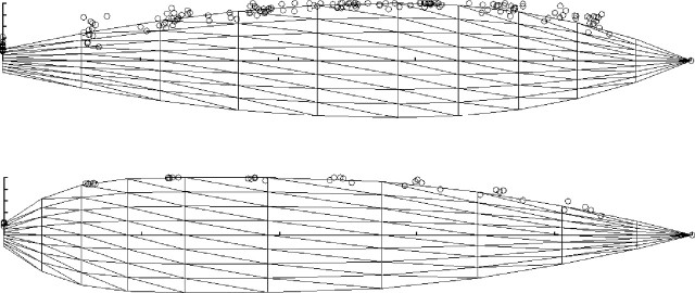
Leaf shape in rice. Change in width of the blade from collar (left) to tip (right). Flag leaves (bottom) were different from all other leaves (top). The families of Hermite function curves show leaf shapes for different lengths during growth. Each circle represents a measurement of a fully expanded blade.
Leaf angles. The axial angle between sheaths and blades of leaves (θ01, Fig. 4) varied with leaf position between 40° and 15° on the main stem, between 75° and 12° in primary tillers, and between 60° and 15° in secondary tillers (Fig. 5). The relationship between θ01 and θ03 (Fig. 4) was fitted empirically by an exponential function (Fig. 6):
 |
and
 |
Fig. 4.

The axial angles, θ01, θ02 and θ03, used to define the curvature of the blade of a leaf. The x, y, z co-ordinates of points P0, P1 and P2 were measured using a 3D digitizer. P1 is the mid-point of the blade and L is the segmented line approximation (P0, P1, P2) to the length of the blade. Arrows show the tangent vectors that were used in the Hermite curve expression.
Fig. 5.
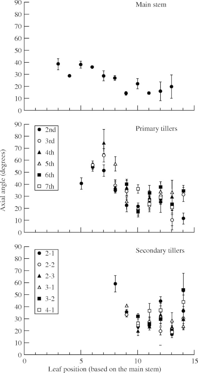
Axial angles between leaf sheaths and blades (θ01, Fig. 4) for different positions on the main stem, primary tillers and secondary tillers. Vertical bars show standard errors. ‘2-1’ means the first secondary tiller of the second primary tiller, and so on.
Fig. 6.

The relationship between leaf blade axial angles θ01 and θ03 (Fig. 4). The line is the curve fitted according to eqn (22).
In the ‘Homomorphism’ pre-defined functions ‘&’ were used to bend each module. The term ‘&(θ)’ means pitch down by angle θ and was used to represent leaf blade curvatures and tiller angles.
It was found that axial curves of leaf blades could be fitted using similar Hermite functions to those used for the shape of leaf margins. However, an appropriate function to describe the angle changes in relation to the node position could not be found, so averaged measured angles at each node (Fig. 4) were used.
Leaf azimuth. Each leaf appears alternately along a stem at a divergence of 180°, with some random azimuth deviations from the standard plane (Fig. 7). Some predefined functions were introduced to eqn (10):
 |
where /(θ) means ‘roll right by angle θ°’ and nran (mean, σ) generates random numbers with normal distribution with mean and standard deviation (σ). The first rotation ‘/(180)’ gives alternate phyllotaxis. The third one ‘/[nran(0,15)]’ represents a random factor of each leaf blade azimuth. The values of mean = 0 and σ = 15 were set empirically, since we have no measurements of the azimuth. The second rotation ‘/(90)’ captures the rotation of the axillary bud.
Fig. 7.
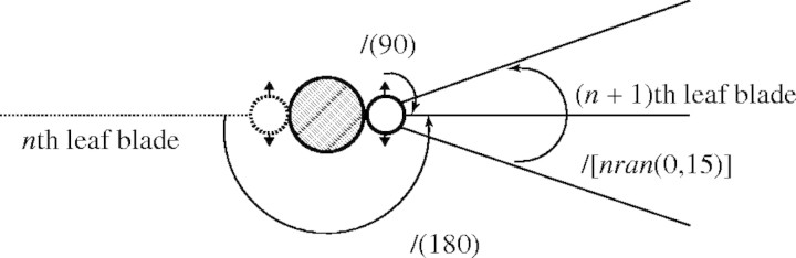
A vertical view of the leaves and axillary buds. Broken and solid lines show the nth and the (n + 1)th leaf blade azimuth standard plane. Each leaf's azimuth has some random deviations, /[nran(0,15)]. Two circles show axillary buds that will produce tillers. Small triangles show the standard azimuth of the leaves produced by the tillers.
Leaf sheath length. There was a linear correlation between the lengths of leaf sheaths and blades (Fig. 8):
 |
Fig. 8.

The relationship between lengths of leaf blades and sheaths.
Since the first leaf of the main stem has no blade (Chang and Bardenas, 1965), n represents positions starting from 1 at the second leaf on the main stem. We assumed a logistic pattern and fitted the same equation (eqn 20) as used for leaf blade length.
 |
where Smax,n is the final sheath length for each leaf position calculated from eqn (25), tsum and D are the same as in the eqn (20). Equation (26) shows that the sheath expansion starts after the leaf blade expansion.
Internode length. The internodes observed to elongate were those between the panicle and flag leaf and the preceding three-to-five internodes beneath. The fully expanded length, Imax,nf, of an internode was found to be a function of internode number, nf (counted from 1 for the first internode to elongate), and the sum of all internode lengths, Itotal (mm):
 |
The length of an expanded internode expressed as a proportion of the sum of all internode lengths, rnf, was fitted by an exponential function (Fig. 9):
 |
Fig. 9.

The relative fully expanded lengths of the final four internodes of the main stem. Internode 4 is between the flag leaf and the panicle. The curved line is fitted according to eqn (28).
Measurements were insufficiently frequent to allow precise estimates of how the rate of internode elongation varied with time. We assumed a logistic pattern and fitted the same eqn (20) as used for leaf blade length:
 |
where Imax,nf is the final internode length at each position, tsum is accumulated d10 from the start of internode elongation, and Dh is the time in d10 from the start of expansion at which Ilen reaches half of the final length. The value of parameter b varies with position:
 |
Since we did not have a good model to estimate the total length of internodes, measured Itotal was used a priori.
Tiller angles. The axial angles of tillers to their parent modules tended to reach a peak about 150–200 d10 after emergence of the tiller and then declined (Fig. 10). The maximum angle of a primary tiller was reduced if it has no secondary tillers. The maximum angles of the 2nd to 4th primary tillers that bore secondary tillers were greater than those of 5th to 7th primary tillers. We measured the angle between the base of tillers and the top position in each tiller using the 3D digitizer (Fig. 11), since internodes were not visible. Therefore, the angle decreased when the internode started to elongate upward.
Fig. 10.

Variation in axial angles between tillers and the main stem with the time since tiller emergence. Vertical bars show s.e.
Fig. 11.

Schematic view of the relationship between the main stem and a tiller. Each box represents an internode. The angle between line segments 0 and 1 shows the maximum angle between the main stem and the primary tiller. The angle between line segments 0 and 2 shows the tiller angle after internode elongation.
In the model, the axial angle, θtill, between a parent module and its daughter tiller increases with the number of tillers produced by the parent module above and on the same side as the daughter tiller, Np, and with the number of tillers produced by the daughter tiller, Nd.
 |
where atill is a constant.
Simulation
The model produced plant architectures for stages from young seedling to maturity (Fig. 12). The processes of panicle ripening and leaf senescence were not parameterized in our experiments. Therefore, functions that respond to cumulative temperature were introduced. The parameters of those functions were determined empirically. We applied the model to reconstruct measured plants growing during September 1997 to January 1998 by using measured average daily temperature and day length. Figure 13 shows the simulated plants and digitized results of the experimental plants at two different growth stages, DVI = 1·6 and 2·4. Simulation results are visually very similar to measured plants.
Fig. 12.

Virtual rice. Images made from 3D representations of rice plant architecture at eight stages of development. DVI is a developmental index running from 0 at emergence of the first leaf to 3·0 when the grains are mature.
Fig. 13.

Simulated plants (first image on left) and digitized plants from the experiment at two growth stages; DVI = 1·6 and 2·4. In the digitized plants, stems and leaves were shown as lines.
The parameter set of ‘Koshihikari’ was applied for the DVI calculation, and that of ‘Nipponbare’ for the leaf development. In this case, measured number of tillers and accumulated number of leaves are well described by the simulated results, even though the simulated leaf number was usually smaller than the measured (Fig. 14).
Fig. 14.
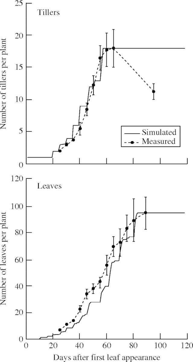
Measured and simulated number of tillers and accumulated number of leaves. Vertical bars show s.e.
The tiller reduction process that is usually observed in rice plant growth was not taken into account in the model. As a consequence, simulated number of tillers showed a constant value after reaching the maximum tillering stage, whereas the observed number of tillers decreased until flowering. The model output underestimated the leaf number, especially during the vegetative stage. That means the actual development of leaves was slightly faster than the simulation output.
DISCUSSION
The 3D ‘virtual rice’ model we developed has a phenological submodel calculating DVI and the timing of leaf emergence. It is, however, still at a primitive stage, especially for morphological differences between varieties, responses to the environmental and biological interaction. In our growth experiment, a single seedling was transplanted in each pot and sufficient nutrients and water were supplied. Therefore, space and/or distance between plants is probably not a growth limitation during the early vegetative stages. The tillering process integrated in our model assumes that tillers emerge at times that follow Katamaya's (1951) synchronous development, and reproduced the tiller number growth, suggesting that tillering pattern of isolated plants can be approximated reasonably well by this simple rule. In actual paddy fields, however, several rice seedlings are transplanted into the same point. Nutrients and space limitation alter the probability of tiller emergence from the axillary bud. Currently, analysis of tiller emergence from a number of field observations is underway and a future version of the tillering model will incorporate axillary bud growth in response to plant density, plant age, temperature and nutrient availability.
Phenological development of the rice plant is represented as an interaction between genetics and environment. We simulated the timing of phenological development (such as panicle initiation, flowering and maturing, and the increase in the tiller number) appropriately in our model. Although we used different cultivars' parameter sets for these calculations, the current attempts may contribute to demonstrate the differences in the structure and development under a wide range of environmental conditions. Parameters for the DVI calculation of many cultivars have been accumulated (Hasegawa et al., 1995; Nakagawa and Horie, 1995; Yajima et al., 1999). Even though only one cultivar and one season of growth data was used to construct our model, this 3D virtual rice can be used for a graphical demonstration of the effects of photoperiod and temperature on the growth of different cultivars in different locations, once the model is linked to different cultivars' DVI data.
In our model, the lengths of fully expanded leaf blades were set a priori. Kaitaniemi et al. (1999, 2000) developed a prediction procedure for the development of following leaves using measurements of the size of previous leaves in sorghum. Similar relationships to those reported by Kaitaniemi et al. were found in our studies (Fig. 1), and may be applied to estimate leaf blade length in rice plants. A few papers have described individual leaf growth, but mainly for the main stem (e.g. Arashi and Eguchi, 1954; Yamazaki, 1964; Hoshikawa, 1975). Tivet et al. (2001) showed leaf growth differences in the main stem and tillers between three varieties, and showed a similar relationship between leaf position and leaf blade length as our results.
We applied Katayama's (1951) leaf growth rule in eqn (12). Simulated leaf number development was slower than that of the real plant (Fig. 14). Some researchers have already pointed out the discrepancy between the ‘synchronous development of leaves and tillers’ theory (Katayama, 1951) and the actual increase in leaves of rice plants (e.g. Matsuba, 1988; Tivet et al., 2001; Goto, 2003). Matsuba (1988) showed that the actual number of leaves on each tiller increased by 0–1 on the primary tillers and 1–2 on the secondary tillers from the expected number of the leaves on each tiller by Katayama's theory. In our experiment, the number of leaves on some primary and secondary tillers was larger by one than on the main stem (Figs 1, 5). These facts may result in an intrinsic error in the total number estimates. Tivet et al. (2001) reported similar results and showed the appearance of leaves on the first primary tiller preceded the appearance of the corresponding leaves on the main stem by 0·5–0·8 phyllochrons in three cultivars. They showed that the sum of leaf index and tiller index, according to Bos and Neuteboom (1998), can standardize the leaf blade length and width growth within primary tillers more simply than Katayama's theory. More information is needed about the relationship between leaf position and leaf size among different cultivars, and about growth changes under different growth conditions, in order to improve the leaf growth sub-model in the 3D virtual rice.
To model the relationships between the relative length and width in the leaves, we applied a Hermite function to express realistic leaf shape and curvature (Fig. 3). Further investigation may be needed to determine the appropriate relationship for other cultivars or in other environmental conditions. We also have to create a more simple procedure to express 3D leaves in the model in order to calculate the distribution of sunlight in the canopy (Chelle and Andrieu, 1998). The simulation results were verified against the measured plants mainly by eye (Figs 12, 13). Finding appropriate measures for validation of 3D virtual plants with real plants' architecture is another area for future research.
Our 3D virtual rice is not linked with physiological processes, such as photosynthesis, and hormonal and nutrient movements. However, our model already has a function of signal transfer by using context-sensitive production rules. In our model, context-sensitive rules only pass information regarding the number of tillers in each node, which is used for the tiller angle calculation (see Appendix), but similar production rules can transfer any information, such as the amount of hormone and nutrients. Each organ has some parameters that show individual information, such as topological connection, accumulated temperature since emergence and physiological age. Therefore, our model has the capability to be linked with a physiological model where each organ calculates information, such as amount of carbohydrate and nitrogen, or light intensity.
Intensive research into the plant genome has generated extensive information on the functions of numerous genes. Sets of genes that determine leaf shape and plant structure have been identified, and the processes and the mechanisms by which genes are expressed in the phenotype have been studied (e.g. Sasaki et al., 2002; Tsukaya, 2002). To allow integration of new information into the virtual rice model, we must provide a user-friendly interface so that any researcher can simulate different types of plant architecture easily. Such a simulator will provide a wide range of ideas for plant breeders and agronomists to investigate with real experiments. It may also allow new experimental approaches, such as using the virtual field to test proposed plant sampling regimes before starting an expensive field study.
The 3D digitizer makes it possible to accumulate information on morphology and architecture from intact plants much easier and faster than previous methods. It is also useful for numerical description of morphological differences between varieties. In spite of this it still took nearly one hour to finish digitizing a rice plant that was fully developed. This was because the increase in the number of leaves measured was exponential (Fig. 14). Aside from geometric data, the digitizing process recorded topological information, order and connection of each organ at the same time. Identification and digitizing every leaf from the dense canopy was laborious work. Leaf shape and curvature are important factors that represent cultivars' character, and allow simulation of the light energy environment in the canopy. The width of a rice leaf, however, is too narrow to digitize accurately with current equipment. Other advanced techniques, such as remote sensing and image processing (e.g. Ivanov et al., 1995; Sinoquet et al., 1998), may be needed to improve labour constraints.
APPENDIX
Within the L-system formalism, context-sensitive production rules can be used to transfer information within the structure. According to Prusinkiewicz and Lindenmayer (1990), the basic syntax of context-sensitive production rules is as follows:
 |
where the a can produce b if, and only if, a is preceded by aleft and followed by aright. The aleft and aright form the left and the right context of a in this production.
To calculate number of tillers, we put insert two marker components, Node and Tiller, into the production rule, eqn (10):
 |
where Node(i, j) stands for each node and Tiller(i,j) represents each tiller. Node and Tiller have no actual (visual) form in the model, but are used to calculate tiller angle (see eqn 31).
The axial angle between a parent module and its daughter tiller increases with the number of tillers produced by the parent module above and on the same side as the daughter tiller, and with the number of tillers produced by the daughter tiller. Context-sensitive rules express this procedure as follows:
 |
 |
 |
 |
When a new apical meristem A emerges, Node(i,j) transfers the information of the number of tillers produced by the daughter tiller, i, and Tiller(i,j) holds the information.
Then a Node(i,j) looks for the information of the number of tillers produced by the parent module above and on the same side as the daughter tiller, j, using the following production:
 |
Tiller(i2,j2) accumulates the information of the total number of tillers, j1 + i2:
 |
This information is then used to calculate the tiller angle. Finally, Node(i,j) resets its information after it has been passed on, and in preparation for recalculation in the next cycle:
 |
Acknowledgments
A part of this work was carried out while T. Watanabe was visiting CSIRO Entomology in Brisbane and was supported by a grant from JST, Japan Science and Technology Agency. Myriam Raymond and Sounthi Subaaharan gave invaluable practical help with the experiment. We thank Robert Williams, Yanco Agricultural Institute, for providing rice seeds, and Shu Fukai, the University of Queensland, for helpful advice on culture techniques. We also thank Geoff Norton and Myron Zalucki for encouraging TW to study in Australia. This study was also partly supported by a Grant-in-Aid (no. 12556004) from the Japanese Ministry of Education, Culture, Sports, Science, and Technology, by a Co-operative Research Programme: Biological Resource Management for Sustainable Agricultural Systems from OECD, and by a Development of Rice Genome Simulators project (no. SY2105) from National Institute of Agrobiological Sciences.
Footnotes
Present address: National Institute for Agro-Environmental Sciences, 3-1-3 Kannondai, Tsukuba, Ibaraki 305-8604, Japan.
Present address: Ishikawa Agricultural College, Nonoichi, Ishikawa-gun, Ishikawa 921-8836, Japan.
LITERATURE CITED
- Arashi K, Eguchi H. 1954. Studies on growth of leaves of paddy rice plant. I. The growth of the leaf-blade and leaf-sheath. Proceedings of the Crop Science Society of Japan 23: 21–25. [Google Scholar]
- Boissard P, Valery P, Akkal N, Helbert J. 1996. Dynamic 3D plant modelling: a morphological and structural approach based upon stereo data acquisition. Aspects of Applied Biology 46: 125–129. [Google Scholar]
- Bos HJ, Neuteboom JH. 1998. Growth of individual leaves of spring wheat (Triticum aestivum L.) as influenced by temperature and light intensity. Annals of Botany 81: 141–149. [Google Scholar]
- Cassman KG, Peng S, Olk DC, Ladha JK, Reichardt W, Dobermann A, Singh U. 1998. Opportunities for increased nitrogen use efficiency from improved resource management in irrigated rice systems. Field Crops Research 56: 7–39. [Google Scholar]
- Chang TT, Bardenas EA. 1965.The morphology and varietal characteristics of the rice plant. Technical Bulletin 4. International Rice Research Institute. [Google Scholar]
- Chelle M, Andrieu B. 1998. The nested radiosity model for the distribution of light within plant canopies. Ecological Modelling 111: 75–91. [Google Scholar]
- Conway, GR. 1997.The doubly green revolution. London: Penguin. [Google Scholar]
- de Reffye P, Houllier F, Blaise F, Barthelemy D, Dauzat J, Auclair D. 1995. A model simulating above- and below-ground tree architecture with agroforestry applications. Agroforestry Systems 30: 175–197. [Google Scholar]
- Dobermann A, Dawe D, Roetter RP, Cassman KG. 2000. Reversal of rice yield decline in a long-term continuous cropping experiment. Agronomy Journal 92: 633–643. [Google Scholar]
- Fischer KS. 1998. Toward increasing nutrient-use efficiency in rice cropping systems: the next generation of technology. Field Crops Research 56: 1–6. [Google Scholar]
- Foley JD, van Dam A, Feiner SK, Hughes JF. 1990.Computer graphics: principles and practice, 2nd edn. Reading, UK: Addison-Wesley. [Google Scholar]
- Fournier C, Andrieu B. 1998. A 3D architectural and process-based model of maize development. Annals of Botany 81: 233–250. [Google Scholar]
- Gao LZ, Jin ZQ, Li L. 1987. Photo-thermal models of rice growth duration for various varietal types in China. Agricultural and Forest Meteorology 39: 205–213. [Google Scholar]
- Goto Y. 2003. Tillering behavior of rice plants. Japanese Journal of Crop Science 72: 1–10. [Google Scholar]
- Graf B, Rakotobe O, Zahner P, Delucchi V, Gutierrez AP. 1990. A simulation model for the dynamics of rice growth and development. Part I . The carbon balance. Agricultural Systems 32: 341–365. [Google Scholar]
- Hanan JS, Room PM. 1997. Practical aspects of virtual plant research. In: Michalewicz MT. ed. Plants to ecosystems : modelling of biological structures and processes. Advances in Computational Life Sciences. Melbourne: CSIRO, 28–44 + Plates 3 & 4. [Google Scholar]
- Hasegawa T, Miyachi Y, Shigaki H, Takano J, Miura M, Sakihara K, Katano M. 1995. Prediction of rice growth and yield based on the weather-crop relation in Kumamoto Prefecture I. Prediction of developmental stages. Proceedings of School of Agriculture Kyushu Tokai University 14: 9–15. [Google Scholar]
- Hasegawa T, Horie T. 1997. Modelling the effect of nitrogen on rice growth and development. In: Kropff MJ, Teng PS, Aggarwal PK, Bouma J, Bouman BAM, Jones JW, van Laar HH, eds. Applications of systems approaches at the field level. Dordrecht: Kluwer, 243–257. [Google Scholar]
- Horie T. 1987. A model for evaluating climatic productivity and water balance of irrigated rice and its application to southeast Asia. Southeast Asia Studies 25: 62–74. [Google Scholar]
- Hoshikawa K. 1975.The growing rice plant, Tokyo: Noubunkyo (Rural Culture Association), 317. (In Japanese). [Google Scholar]
- Hyams DG. 1997.CurveExpert 1.3 A comprehensive curve fitting system for Windowshttp://curveexpert.webhop.biz/ (accessed March 2004). [Google Scholar]
- Ito A. 1969. Geometrical structure of rice canopy and penetration of direct solar radiation. Proceedings of the Crop Science Society of Japan 38: 355–363. [Google Scholar]
- Ito A, Udagawa T, Uchijima Z. 1973. Phytometrical studies of crop canopies II. Canopy structure of rice crops in relation to varieties and growing stage. Proceedings of the Crop Science Society of Japan 42: 334–342. [Google Scholar]
- Ivanov N, Boissard P, Chapron M, Andrieu B. 1995. Computer stereo plotting for 3D reconstruction of a maize canopy. Agricultural and Forest Meteorology 75: 85–102. [Google Scholar]
- Kaitaniemi P, Room PM, Hanan JS. 1999. Architecture and morphogenesis of grain sorghum, Sorghum bicolor (L.) Moench. Field Crops Research 61: 51–60. [Google Scholar]
- Kaitaniemi P, Room PM, Hanan JS. 2000. Virtual sorghum: visualisation of portioning and morphogenesis. Computers and Electronics in Agriculture 28: 195–205. [Google Scholar]
- Katayama T. 1951.Studies on tillering of rice, wheat and barley. Tokyo: Yokendo. [Google Scholar]
- Kawahara H, Chonan N, Wada K. 1968. Studies on morphogenesis in rice plants. 3. Interrelation of the growth among leaves, panicle and internodes, and a histological observation on the meristem of culm. Proceedings of the Crop Science Society of Japan 37: 372–383. [Google Scholar]
- Khush GS. 1996. Prospects of and approaches to increasing the genetic yield potential of rice. In: Evenson RE, Herdt RW. Hossain M. eds. Rice research in Asia. Progress and priorities. Wallingford, UK: CAB International, 59–71. [Google Scholar]
- Khush GS, Virk PS. 2002. Rice improvement: past, present and future. In: Kang MS, ed. Crop improvement: challenges in the twenty-first century. New York: Food Products Press, 17–42. [Google Scholar]
- Kropff MJ, van Laar HH, Matthews RB. 1994.ORYZA1: An ecophysiological model for irrigated rice production. SARP Research Proceedings, Manila: International Rice Research Institute. [Google Scholar]
- Ladha JK, Kirk GJD, Bennett J, Peng S, Reddy CK, Reddy PM, Singh U. 1998. Opportunities for increased nitrogen-use efficiency from improved lowland rice germplasm. Field Crops Research 56: 41–71. [Google Scholar]
- Lindenmayer A. 1968. Mathematical models for cellular interactions in development, Parts I and II. Journal of Theoretical Biology 18: 280–315. [DOI] [PubMed] [Google Scholar]
- Mabrouk H, Carbonneau A, Sinoquet H. 1997. Canopy structure and radiation regime in grapevine. 1. Spatial and angular distribution of leaf area in two canopy systems. Vitis 36: 119–123. [Google Scholar]
- Matsuba K. 1988. Morphological studies on the regularity of shoots development in rice plants. II. Regularity in tillering termination and the maximum number of tillers. Japanese Journal of Crop Science 57: 599–607. [Google Scholar]
- Mech R. 1998.CPFG Version 3.4 User's Manual http://www.cpsc.ucalgary.ca/Research/bmv/lstudio/manual.pdf (accessed March 2004). [Google Scholar]
- Mech R, Prusinkiewicz P, Hanan J. 1997.Extensions to the graphical interpretation of L-system based on turtle geometry http://www.cpsc.ucalgary.ca/Research/bmv/lstudio/graph.pdf (accessed March 2004). [Google Scholar]
- Miglietta F. 1991. Simulation of wheat ontogenesis. I. Appearance of main stem leaves in the field. Climate Research 1: 145–150. [Google Scholar]
- Nakagawa H, Horie T. 1991. Modelling and prediction of developmental process in rice. 10. Model for predicting development in leaf number. Japanese Journal of Crop Science 60: 272–273. [Google Scholar]
- Nakagawa H, Horie T. 1995. Modelling and prediction of developmental process in rice II. A model for simulating panicle development based on daily photoperiod and temperature. Japanese Journal of Crop Science 64: 33–42. [Google Scholar]
- Peng S, Khush GS, Cassman KG. 1994. Evolution of the new plant type for increased yield potential. In: Cassman, KG. ed. Breaking the yield barrier: proceedings of a workshop on rice yield potential in favourable environments Manila: International Rice Research Institute, 5–20. [Google Scholar]
- Penning de Vries FWT, Jansen DM, ten Berge HFM, Bakema A. 1989.Simulation of ecophysiological processes of growth in several annual crops. Wageningen: Pudoc. [Google Scholar]
- Perttunen J, Sievanen R, Nikinmaa E. 1998. Lignum – a model combining the structure and the functioning of trees. Ecological Modelling 108: 189–198. [Google Scholar]
- Prusinkiewicz P, Hanan J. 1989.Lindenmayer systems, fractals, and plants. Volume 79 of Lecture notes in Biomathematics. Berlin: Springer-Verlag. [Google Scholar]
- Prusinkiewicz P, Hanan JS, Mech R. 2000. An L-system-based plant modeling language. In: Nagl M, Schurr A, Munch M, eds. Lecture notes in computer science 1779: applications of graph transformation with industrial relevance. Berlin: Springer-Verlag, 395–410. [Google Scholar]
- Prusinkiewicz P, Lindenmayer A. 1990.The algorithmic beauty of plants. New York: Springer-Verlag. [Google Scholar]
- Ritchie JT, Alocilija EC, Singh U, Uehara G. 1987. IBSNAT and the CERES-Rice model. Proceedings of the Workshop on the Impact of Weather Parameters on Growth and Yield of Rice April 1986. Manila: International Rice Research Institute, 271–281. [Google Scholar]
- Room PM, Hanan JS, Prusinkiewicz P. 1996. Virtual plants: new perspectives for ecologists, pathologists and agricultural scientists. Trends in Plant Science 1: 33–38. [Google Scholar]
- Room PM, Maillette L, Hanan JS. 1994. Module and metamer dynamics and virtual plants. Advances in Ecological Research 25: 105–157. [Google Scholar]
- Sasaki A, Ashikari M, Ueguchi-Tanaka M, Itoh H, Nishimura A, Swapan D et al. 2002. A mutant gibberellin-synthesis gene in rice. Nature 416: 701–702. [DOI] [PubMed] [Google Scholar]
- Sattler R, Rutishauser R. 1997. The fundamental relevance of morphology and morphogenesis to plant research. Annals of Botany 80: 571–582. [Google Scholar]
- Sheehy JE, Dionora MJA, Mitchell PL, Peng S, Cassman KG, Lemaire G, Williams RL. 1998. Critical nitrogen concentrations: implications for high-yielding rice (Oryza sativa L.) cultivars in the tropics. Field Crops Research 59: 31–41. [Google Scholar]
- Shibayama M. 2001. Estimation of leaf area and leaf inclination distributions of perennial ryegrass, tall fescue, and white clover canopies using an electromagnetic 3-D digitizer. Grassland Science 47: 303–306. [Google Scholar]
- Sinoquet H, Moulia B, Bonhomme R. 1991. Estimating the three-dimensional geometry of a maize crop as an input of radiation models: comparison between three-dimensional digitizing and plant profiles. Agricultural and Forest Meteorology 55: 233–249. [Google Scholar]
- Sinoquet H, Thanisawanyanggkura S, Mabrouk H, Kasemsap P. 1998. Characterisation of the light environment in canopies using 3-D digitising and image processing. Annals of Botany 82: 203–212. [Google Scholar]
- Takenaka A, Inui Y, Osawa A. 1998. Measurement of three-dimensional structure of plants with a simple device and estimation of light capture of individual leaves. Functional Ecology 12: 159–165. [Google Scholar]
- Tanaka T, Matsushima S, Kojo S, Nitta H. 1969. Analysis of yield-determining process and its application to yield prediction and culture improvement of lowland rice. XC. On the relation between the plant type of rice plant community and the light-curve of carbon assimilation. Proceedings of the Crop Science Society of Japan 38: 287–293. [Google Scholar]
- Tivet F, Pinheiro BDS, Raissac MD, Dingkuhn M. 2001. Leaf blade dimensions of rice (Oryza sativa L. and Oryza glaberrima Steud.). Relationships between tillers and the main stem. Annals of Botany 88: 507–511. [Google Scholar]
- Tsukaya H. 2002. Leaf development. In:Somerville CR, Meyerowitz EM, eds. The Arabidopsis book. Rockville, MD American Society of Plant Biologists. /10·1199/tab.0072, http://www.aspb.org/downloads/arabidopsis/tsukayafinal.pdf [Google Scholar]
- Tsunoda S. 1959. A developmental analysis of yielding ability in varieties of field crops. II. The assimilation-system of plants as affected by the form, direction and arrangement of single leaves. Japanese Journal of Breeding 9: 237–244. [Google Scholar]
- Udagawa T, Ito A, Uchijima Z. 1974a. Phytometrical studies of crop canopies III. Radiation environment in rice canopies. Proceedings of the Crop Science Society of Japan 43: 180–195. [Google Scholar]
- Udagawa T, Ito A, Uchijima Z. 1974b. Phytometrical studies of crop canopies IV. Structure of canopy photosynthesis of rice plants. Proceedings of the Crop Science Society of Japan 43: 196–206. [Google Scholar]
- Wu GW, Wilson LT. 1998. Parameterization, verification, and validation of a physiologically complex age-structured rice simulation model. Agricultural Systems 56: 483–511. [Google Scholar]
- Yajima M, Terashima K, Maruyama S. 1999. DVR parameters of leading rice varieties in Japan. Japanese Journal of Crop Science 68: 64–65. [Google Scholar]
- Yamazaki K. 1964. Studies on leaf formation in rice plants. III. Effects of some environmental conditions on leaf development. Proceedings of the Crop Science Society of Japan 32: 145–151. [Google Scholar]
- Yin XY, Kropff MJ. 1996. The effect of temperature on leaf appearance in rice. Annals of Botany 77: 215–221. [Google Scholar]