Genecology of Douglas Fir in Western Oregon and Washington

Abstract

• Background and Aims Genecological knowledge is important for understanding evolutionary processes and for managing genetic resources. Previous studies of coastal Douglas fir (Pseudotsuga menziesii var. menziesii) have been inconclusive with respect to geographical patterns of variation, due in part to limited sample intensity and geographical and climatic representation. This study describes and maps patterns of genetic variation in adaptive traits in coastal Douglas fir in western Oregon and Washington, USA.

• Methods Traits of growth, phenology and partitioning were measured in seedlings of 1338 parents from 1048 locations grown in common gardens. Relations between traits and environments of seed sources were explored using regressions and canonical correlation analysis. Maps of genetic variation as related to the environment were developed using a geographical information system (GIS).

• Key Results Populations differed considerably for adaptive traits, in particular for bud phenology and emergence. Variation in bud-set, emergence and growth was strongly related to elevation and cool-season temperatures. Variation in bud-burst and partitioning to stem diameter versus height was related to latitude and summer drought. Seedlings from the east side of the Washington Cascades were considerably smaller, set bud later and burst bud earlier than populations from the west side.

• Conclusions Winter temperatures and frost dates are of overriding importance to the adaptation of Douglas fir to Pacific Northwest environments. Summer drought is of less importance. Maps generated using canonical correlation analysis and GIS allow easy visualization of a complex array of traits as related to a complex array of environments. The composite traits derived from canonical correlation analysis show two different patterns of variation associated with different gradients of cool-season temperatures and summer drought. The difference in growth and phenology between the westside and eastside Washington Cascades is hypothesized to be a consequence of the presence of interior variety (P. menziessii var. glauca) on the eastside.

INTRODUCTION

Describing and understanding the geographical structure of genetic variation and its relation to environments are important for understanding evolutionary processes and for managing our heritage of genetic resources. Correlations between genetic variation and environmental differences among seed sources suggest natural selection and adaptation of genotypes to their environments, particularly when the correlations make sense physiologically (Heslop-Harrison, 1964; Endler, 1986). Mapped genetic variation and an understanding of natural genetic structure are used to develop guidelines for seed movement in reforestation, for managing breeding populations in advanced generation breeding programmes, for evaluating conservation of genetic resources, and for predicting and possibly mitigating effects of climate change. Furthermore, knowledge of geographical variation among populations of outcrossing, undomesticated conifers may contribute substantially to exploring the molecular basis of quantitatively inherited adaptive traits through association genetics studies (Neale and Savolainen, 2004).

Douglas fir (Pseudotsuga menziesii) is one of the most ecologically and economically important trees in western North America, and is planted as an exotic timber species in Europe, New Zealand, Australia and Chile. It has one of the widest natural ranges of any tree species, extending from the Pacific Coast to the eastern slope of the Rocky Mountains and from 19°N in Mexico to 55°N in western Canada (Hermann and Lavender, 1990). Two varieties are recognized: P. menziesii var. menziesii, called coastal Douglas fir and found along the North American Pacific Coast (California, Oregon, Washington and British Columbia), and P. menziesii var. glauca, called Rocky Mountain or interior Douglas fir and found inland in the mountains from British Columbia to central Mexico. Within a region, Douglas fir can grow under a wide variety of climatic conditions; in western Oregon and Washington, it occurs from sea level to over 1700 m.

Compared with many tree species, Douglas fir populations are generally regarded as being closely adapted to their environments with relatively steep clines associated with steep environmental gradients (Rehfeldt, 1994). Results from nursery common garden studies with seedlings indicate that genetic variation in growth, germination and bud phenology follows a clinal pattern with steep clines mainly occurring along elevational gradients, but also related to aspect, slope, latitude, longitude and distance to the ocean (Hermann and Lavender, 1968; Griffin and Ching, 1977; Campbell and Sorensen, 1978; Griffin, 1978; Campbell, 1979, 1986; Rehfeldt, 1979, 1982, 1983, 1989; Sorensen, 1983; Campbell and Sugano, 1993). Results after 25 years from a coastal Douglas fir provenance study, however, seem to contradict the findings from seedling genecology studies (White and Ching, 1985). Despite significant differences among 14 provenances from a wide geographical region planted at five sites from British Columbia to California, the provenance by planting location interaction was non-significant and small. Their study, however, suffers the same drawbacks of many provenance studies, namely a limited number of populations from a limited number of source environments planted over a limited number of test sites. Small sample sizes make it difficult to study the relationship between genetic variation and environmental differences where environmental gradients are complex and highly heterogeneous, and extrapolation of results to a wider range of environments is often not possible. Furthermore, seed for each population may have come from a large area relative to areas within which considerable genetic differentiation may occur (e.g. Campbell, 1979), resulting in population buffering and a reduced likelihood of finding a provenance-by-location interaction.

Results from field tests of tree improvement programmes have also provided insight into the structure of genetic variation of coastal Douglas fir. Stonecypher et al. (1996) summarized genetic tests established on lands owned by Weyerhaeuser Company in western Oregon and Washington that were designed to explore questions of genotype-by-environment interaction. They concluded that family-by-planting location interaction was small relative to family and planting location effects, and where significant, was predominately the result of a few families. Johnson (1997) considered genetic correlations among test sites in six breeding zones in Oregon and concluded that breeding zones were not particularly large given that site-to-site genetic correlations were relatively strong and were unrelated to the differences among sites in elevation, latitude or longitude. In contrast to these results, Campbell (1992), using a different analytical approach, found significant family-by-site interaction in several breeding zones in Oregon. Similarly, Silen and Mandel (1993) showed clinal variation in height growth based on results from progeny tests in two breeding zones in Oregon. All of these studies, however, were designed with specific objectives of managing variation within tree improvement programmes, and, therefore, were limited in geographical range and the range of genotypes and environmental conditions sampled. They were not designed to provide a systematic sample of environmental conditions of seed sources and planting locations across the ranges of natural variation in each to explore adequately the relationship between genetic variation and environments.

The objectives of this study are: (1) to describe and map patterns of genetic variation in coastal Douglas fir in western Oregon and Washington; and (2) to determine the environmental factors that are most strongly related to genetic variation in adaptive traits. The methodology for mapping genetic variation relies on deriving a response surface in which the response of a trait for a genotype from a source location is a function of the environment at the location. Environment is measured directly as climate or measured indirectly by geographical or topographical variables. Response surfaces are best modelled by sampling the independent variables evenly across the range of interest. This is accomplished by a systematic sample on a geographical grid with attention paid to sampling contrasting elevations within the grid. Sample intensity depends upon the environmental variation within a region. More samples per area are required, for example, in the environmentally heterogeneous western North America as compared with the more homogeneous eastern or southern United States. This approach to mapping genetic variation was developed by Campbell (1979, 1986). His approach utilizes open-pollinated seed from a single parent at most locations, and duplicate samples at some locations in order to test lack of fit of the models and to estimate family within-population variances for estimating risks from moving genotypes. His studies of coastal Douglas fir, however, were of limited geographical range (Campbell, 1986; Campbell and Sugano, 1993), and the models used geographical and topographical variables as surrogates for environments at source locations. Climate models have since been developed that provide reliable estimates of climate at each location (Daly et al., 1994). Better climate data improve the models of genetic variation as a function of the environments at source locations, and provide greater insight into the environmental factors that shape genetic structure through natural selection. Furthermore, a larger geographical scale is needed to explore the implications of climate change for adaptation of Douglas fir to future climates. This study considers genetic variation of growth and adaptive traits as a function of environments over the whole range of coastal Douglas fir in western Oregon and Washington using a sampling strategy that is both extensive and intensive. A geographical information system (GIS) is used to display the response surface as a map of genetic variation.

MATERIALS AND METHODS

Sampling from natural populations

Wind-pollinated seed was collected from 1338 parent trees of Douglas Fir [Pseudotsuga menziesii (Mirb.) Franco var. menziesii] in naturally regenerated stands at 1048 locations in western Oregon and Washington (Fig. 1). Most of the seed was obtained from previous collections of the USDA Forest Service, USDI Bureau of Land Management, Oregon Department of Forestry and Northwest Tree Improvement Cooperative. In 1993 and 1995, seed was collected from an additional 231 parents to cover areas not sampled by the other collections. The range of coastal Douglas fir in western Oregon and Washington was well sampled, although sampling intensity was lower along the Washington coast and in urban and agricultural areas around Puget Sound and Willamette Valley. At 291 locations (28 %), cones were collected from two parent trees from the same elevation and aspect, but separated by at least 100 m. These paired samples were used to estimate average variance among families within locations and to test lack of fit to our genecological models.

Fig. 1.

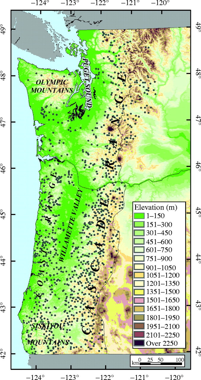
Study area and locations of parents (grey dots).

The environments of seed source locations were characterized using geographical, topographical and climatic data. The geographical and topographical data were obtained from GIS coverages using a 90-m digital elevation model (DEM). Variables included latitude, longitude, linear distance to the sea, elevation, slope, aspect and sun exposure on 21 March (an integrative function of latitude, aspect, slope and local topography). Climatic data were obtained from GIS coverages generated from PRISM (Parameter-Elevation Regressions on Independent Slopes Model), a statistical–geographical model in which climate parameters are predicted for 4 × 4 km grid cells using localized regression equations of climate as a function of elevation with greater weight given to climate data from nearby weather stations of similar elevation and topographical position (Daly et al., 1994; see www.ocs.orst.edu/prism/prism_new.html). PRISM has been used extensively to map precipitation and temperature in the United States, Canada and other countries, and is particularly well suited to mountainous terrain. Climate data are based on the averages for the years 1961–1990. Climate values at specific parent tree locations are determined as distance-weighted averages of the four nearest grid cells using the LATTICESPOT function with the bilinear interpolation option in ARC/INFO. Climate variables included monthly, seasonal and annual averages for minimum and maximum temperature, precipitation, daily temperature fluctuation and aridity (a ratio of precipitation to temperature); dates of 50 % probability of last spring frost and first autumn frost; frost-free period; and seasonal ranges in temperature and precipitation.

Common garden procedures

Breeding values of parent trees were estimated by growing seedlings in a common garden. Seeds were stratified at 3 °C for approximately 60 d before sowing in April in raised nursery beds in Corvallis, Oregon. To evaluate a large number of parent trees, tests were established in three successive years (1994–1996) using different sets of families. Because it was not possible to assign families to sowing years such that sowing years contained an equivalent sampling across the study area, 66 families from 50 well-distributed locations were included in all three sowing years. These families served as a genetic checklot to allow for adjustment of year effects (White and Hodges, 1989; Rehfeldt, 1989). Each year families were randomly assigned to five-tree row plots (12 cm between rows and 7 cm between seedlings) in each of four raised beds with each bed treated as a block. In order to evaluate differences in rate of emergence, four seeds were sown per position for a total of 20 seeds per plot; seedlings were later systematically thinned to one per position.

Seedlings were grown for 2 years during which they were measured for traits of emergence, bud phenology, growth and partitioning (Table 1). Mean rate and standard deviation of the rates of emergence were determined following procedures given in Campbell and Sorensen (1979) based on the cumulative number of seedlings out of 20 that emerged in a plot. Height and bud-set were measured at the end of the first growing season. Bud-set was measured weekly as the number of days since 1 January that terminal bud scales were first visible following any second flushes. At the beginning of the second growing season, bud-burst was measured twice a week as the number of days since 1 January that green needles were first visible emerging from the terminal bud. At the end of the second growing season, bud-set was again measured. Whole seedlings were harvested by carefully excavating the soil from around the roots. Seedlings were measured for stem diameter (1 cm above the root collar), height from root collar to terminal bud, height to the bud-scar resulting from second flushing and length of the longest root. Dry weights of shoots and roots were determined after drying the seedlings at 80 °C for 24 h.

Table 1.

Description of measured and derived traits

Trait	Abbreviation	Description	Units
Shoot weight	SHWT	Dry weight after 2 years	g
Root weight	RTWT	Dry weight after 2 years	g
Total weight	TOTWT	Sum of shoot and root weight	g
First-year height	HT1	From root collar to base of terminal bud	cm
Second-year height	HT2	From root collar to base of terminal bud	cm
Height increment	HTINC	Second-year height minus first-year height	cm
Second-year stem diameter	DIA	At 1 cm above root collar after 2 years	mm
Root length	RTLG	From root collar to tip of longest root	mm
Root : shoot ratio	RTSH	Ratio of dry weights after 2 years	g g −1
Taper	TAPER	Ratio of second-year diameter to second-year height	mm cm −1
First-year bud-set	BS1	First visible terminal-bud scales at end of first growing season	days since 1 January
Second-year bud-set	BS2	First visible terminal-bud scales at end of second growing season	days since 1 January
Second-year bud-burst	BB2	First green needles from terminal bud	days since 1 January
Rate of emergence	EM	Cumulative number of seedlings emerged in a plot on a probit scale	probits d−1
Propensity to second flush	FLUSH	Proportion of 2-year seedlings with lammas growth of terminal leader	proportion
Length of second flush	FLLG	Distance from visible bud scar to base of terminal bud	cm

Analysis

To avoid problems with families from different regions being tested in different years, year-to-year environmental differences were removed from the data by standardizing plot means such that the means and standard deviations for the checklot were equal across years. Analyses of variance and genetic correlations among years using just the data from the checklot families indicated that locations and families-within-locations did not show a differential response to years; location-by-year and family-by-year interactions were not significant and genetic correlations between years were high for all traits and approached one for many traits.

For each trait, components of variance were estimated using the model:

where Y_ijkl is the plot mean performance of the lth family (F) from the kth source location (L) in the jth replication (R) sown in the ith year (Y), μ is the overall experimental mean, and e is the experimental error consisting of the pooled interactions of both sources and families by replications. Year effects have been removed by the standardizing procedure described above and are not included in the model. Source locations and families were treated as random effects. Location differences were tested using families within locations as the error term, and family differences were tested against the experimental error term. Random effects were tested using PROC GLM of the SAS statistical package (SAS Institute Inc., 1999). Variance components were obtained using PROC MIXED.

Relationships between traits and environments at source locations were investigated by correlation, regression and canonical correlation analysis (CCA). Individual traits were regressed on environmental variables using the RSQUARE model-selection method in SAS (SAS Institute Inc., 1999). Individual traits and environmental variables were combined into a few uncorrelated traits and uncorrelated environmental variables using CCA. CCA determines pairs of linear combinations, termed canonical variables, from two sets of original variables, in this case traits and environments, such that the correlation between canonical variables is maximized and subsequent pairs are uncorrelated with previously derived linear combinations (Cooley and Lohnes, 1971; Mardia et al., 1979). It is essentially an extension of multiple regression in which both dependent and independent variables are linear combinations of the original variables. CCA was performed between traits and all geographical, topographical and climatic variables (71 variables) using the CANCORR procedure in SAS. The number of environmental variables was then reduced to avoid including highly correlated, redundant variables by using multiple regression (R-square selection method of the PROC REG procedure in SAS) to determine which variables contributed the most to explaining variation in the first few canonical variables for traits, keeping those variables, and re-running the CCA. Different models were judged based on canonical redundancy analysis, in which redundancy measures the total variation explained and is defined as the product of the proportion of variance extracted by a given linear combination and the proportion of variance shared between pairs of linear combinations (i.e. the square of the canonical correlation) (Cooley and Lohnes, 1971). The criterion for adding an additional variable to the model was an improvement in the redundancy value of at least 0·5 %.

After performing the analysis using all families from all locations, we determined from graphs and residuals from the models that parents from the eastside Washington Cascades were related to the environment differently than other sources, and the difference across the Cascade crest (above 46·5°N) appeared discontinuous (i.e. ecotypic rather than clinal). Because of the discontinuous nature of the variation, we excluded parents from the eastside Washington Cascades from the model developed for the rest of the region; the final model utilized 1256 parents from 985 sources. All steps in the analysis described above were repeated. Differences in the relationships of traits and environments between the eastside and westside Washington Cascades were explored with regressions and correlations.

Models of traits as related to environments were tested for lack of fit using variation among families within locations as pure error (Neter and Wasserman, 1974). Lack of fit is caused by location variation that is not explained by the selected model. Significant lack of fit may be due to unaccounted site factors, such as soils, biotic interactions or microclimate, to non-uniform patterns of gene flow, or to local patterns of variation that differ from the broad-scale, overall pattern of variation.

We also considered the approach taken by Campbell (1979, 1986) and others in subsequent studies in which principal component analysis was first performed on the set of traits followed by multiple regression of factor scores on the environmental variables. Results from the principal component approach were similar to those of the canonical correlations approach, and are not presented (see also Wartenberg, 1985). CCA was preferred because maximizing the correlation between traits and environments is of primary interest in genecology studies.

Mapping procedures

After a final set of traits and environmental variables was selected using CCA, we regressed the canonical scores for traits on the set of environmental variables to generate a predictive model of canonical scores for traits. Regression equations of canonical scores for traits, as well as regression equations of individual traits, were used to map genetic variation as a function of the environment at each grid cell in a GIS using grid algebra functions in ARC/INFO. We resampled 90-m elevation and 4-km climate data to a common 1 × 1 km grid cell size using the ARC/INFO RESAMPLE function with the bilinear interpolation option. Areas above 1700 m are not included because Douglas fir rarely occurs above that elevation. A contour interval was selected for the genetic maps that corresponds to a level of risk of maladaptation of 30 %. Risk of maladaptation is defined as the difference between the frequency distributions for additive genetic variances of a population of seedlings at a source location and a population of seedlings native to the planting site (described in Campbell, 1986). Thus, if seedlings were transferred a distance of one contour interval on the genetic map, 30 % of the seedlings might be expected to be at risk of poor growth and survival relative to the native population. This approach assumes that the native population is optimally adapted to the local environment. Although this assumption may not be strictly true, risk of maladaptation is nevertheless a valuable metric of population differentiation that takes into account mean differences as well as within-population variation. A risk of maladaptation of 30 % is assumed to be an acceptable level of risk for a single trait (Sorensen, 1992).

The derived genetic map describes the overall pattern of genetic variation as predicted by the environment. Actual genetic variation may differ from the predicted variation owing to sampling error, genetic drift, gene flow from adjacent populations, or different, smaller-scale local environmental factors determining natural selection. Local patterns of genetic variation were explored by looking at geographical patterns of residuals from the overall model. Residuals were determined for each source location and mapped using a kriging function in ARC/INFO. Kriging is a geostatistical procedure that generates a surface of estimated values from a scattered set of points using spatial autocorrelation (Cressie, 1991).

RESULTS

Genetic variation among locations and among families within locations

Analyses of variance indicated that differences among families-within-seed source locations were highly significant (P < 0·001) for all traits, and differences among locations were highly significant for all traits except root length (RTLG; P = 0·05), propensity to second flush (FLUSH; P = 0·04) and length of second flushes (FLLG; P = 0·11) (Table 2). The percentage of variation accounted for by differences among locations and families-within-locations differed among traits (Table 2). Rate of emergence (EM), bud-burst (BB2) and first-year bud-set (BS1) had particularly high percentages of location variation. By contrast, second flushing traits (FLUSH, FLLG), root length (RTLG) and partitioning to roots versus shoots (RTSH) had low percentages of both location and families-within-location variation. Growth and size traits exhibited an intermediate level of variation among locations and among families-within-locations.

Table 2.

Results from analyses of variance for original traits and the first two canonical variables for traits(TRAIT1 and TRAIT2)

					Percentage of total variance
Trait†	Overall mean	F-value for locations	F-value for families-within-locations	Total variance	Location	Family	Error
SHWT	9·3	1·58***	2·37***	9·960	16·8	18·9	64·3
RTWT	3·4	1·46***	2·32***	0·915	14·3	18·5	67·1
TOTWT	12·7	1·57***	2·44***	15·842	16·9	19·6	63·4
HT1	12·7	1·31***	3·26***	3·782	13·3	26·1	60·5
HT2	34·7	1·77***	1·95***	41·120	17·9	13·4	68·7
HTINC	22·0	1·86***	1·59***	28·43	17·4	8·9	73·8
DIA	6·3	1·58***	2·47***	0·777	17·1	18·6	64·3
RTLG	33·9	1·18*	1·51***	0·950	5·2	8·0	86·7
RTSH	0·40	1·45***	1·34***	0·0062	8·9	6·6	84·5
TAPER	0·19	1·86***	1·47***	0·000584	17·0	6·5	76·5
BS1	274	2·73***	2·44***	82·00	36·3	14·6	49·1
BS2	223	2·00***	1·50***	30·7·18	18·6	7·9	73·5
BB2	106	2·10***	3·82***	25·94	34·5	21·9	43·6
EM	0·047	2·98***	4·50***	0·0000171	48·5	21·1	30·4
FLUSH	0·37	1·19*	1·35***	0·0703	2·9	7·5	89·6
FLLG	3·0	1·13	1·24***	6·502	2·2	5·2	92·5
TRAIT1	0·0	4·75***	2·40***	1·416	55·3	10·6	34·1
TRAIT2	0·0	2·83***	2·27***	1·681	37·9	13·7	48·4

^†See Table 1 for trait codes and units of measurement.

^*P = 0·05–0·01;

^***P < 0·001.

Relationship between traits and the environments of seed sources

Results from CCA indicate that traits measured in the common garden study were strongly related to the environment of the seed source. The canonical correlation between the first pair of canonical variables was 0·82 (R² = 0·68) and between the second pair was 0·70 (R² = 0·50) (Table 3). Canonical redundancy analysis indicated that the first two canonical correlations accounted for 20 and 7 % of the total variation in the trait data, respectively, whereas subsequent correlations accounted for 1 % or less of the variation (Table 3). For this reason, we considered only the first two pairs of composite traits and environments in subsequent analyses.

Table 3.

Redundancy from canonical correlation analysis

Canonical variable pair	Canonical R2	Proportion of trait variance explained by canonical variable for traits	Proportion of trait variance explained by canonical variable for environments
1	0·68	0·30	0·20
2	0·50	0·15	0·07
3	0·11	0·13	0·01
4	0·06	0·10	0·01
5	0·02	0·04	<0·01

Eleven trait variables were included in the canonical variables for traits; root length and second flushing traits were excluded from the analysis because of low variation among locations. Correlations between the canonical variables for traits and the original trait variables indicated that higher values for the first canonical variable for traits (TRAIT1) were related to vigour, i.e. later bud-set, faster emergence, larger seedling sizes and increased partitioning to shoots versus roots (Table 4). Higher values for the second canonical variable for traits (TRAIT2) were related to earlier bud-burst and greater partitioning to second-year diameter versus height. Nine environmental variables were included in the canonical variables for environment, as well as the corresponding regression models (Table 5). Including all 71 environmental variables only marginally improved the proportion of variance explained (from 0·202 to 0·214 for the first pair of canonical variables and from 0·073 to 0·089 for the second pair).

Table 4.

Correlations between canonical variables for traits and original trait variables

Original variable*	TRAIT1	TRAIT2
SHWT	0·52	0·27
RTWT	0·40	0·32
TOTWT†	0·50	0·29
HT1	0·35	0·43
HT2†	0·56	0·05
HTINC	0·57	−0·21
DIA	0·41	0·43
RTSH	–0·50	–0·11
TAPER	–0·39	0·56
BS1	0·88	0·23
BS2	0·80	–0·01
BB2	0·14	–0·74
EM	–0·64	0·35

^*See Table 1 for trait codes and units of measurement.

^†Not included in the canonical correlation analysis since the trait is a linear combination of other trait variables in the analysis.

Table 5.

Regression equations used in mapping canonical scores for trait given environmental data^*for a location

	TRAIT1			TRAIT2
Independent variable	Regression coefficient	P-value	Regression coefficient	P-value
Intercept	−3·72476	0·0239	18·34020	<0·0001
ELEV	−0·00112	<0·0001	−0·00033	0·0106
SPRFRST	−0·01343	<0·0001	−0·02281	<0·0001
JULPRE	−0·0085	0·0111	0·00116	0·7814
AUGPRE	0·02117	<0·0001	0·00071	0·8768
FEBMXT	0·17083	<0·0001	−0·15134	<0·0001
MAYMXT	−0·15879	<0·0001	−0·0092	0·8514
LAT	0·09134	0·0044	−0·35691	<0·0001
SEPPRE	−0·00032	0·8568	−0·00815	0·0003
JULMXT	0·11432	0·0002	0·10748	0·0045

Probability of lack of fit for TRAIT1 is <0·0001 (F = 2·44); R² = 0·68.

Probability of lack of fit for TRAIT2 is <0·0001 (F = 2·33); R² = 0·50.

^*Key to environmental variables: ELEV = elevation, SPRFRST = date of first spring frost, JULPRE = July precipitation, AUGPRE = August precipitation, FEBMXT = February average maximum daily temperature, MAYMXT = May average maximum daily temperature, LAT = latitude, SEPPRE = September precipitation, JULMXT = July average maximum daily temperature.

TRAIT1 was most strongly related to temperature, particularly minimum temperature in late autumn and winter months (Table 6), and variables that are highly correlated with temperature such as elevation and dates of first spring and last autumn frost (Table 7). Seedlings that were larger, emerged faster, set bud later and partitioned more to shoots versus roots came from warmer areas. The relation between TRAIT1 and elevation is particularly strong (Table 7; Fig. 2). The relation is moderately but significantly (P < 0·001) better modelled as a quadratic equation (R² = 0·57) instead of a linear equation (R² = 0·56); thus, the risk of moving sources between elevations is greater at higher elevations than at lower elevations. For a maximum level of risk of 30 %, seed sources at 200 m elevation may be moved a difference of up to 427 m, whereas seed sources at 1200 m elevation may be moved a difference of up to 243 m.

Table 6.

Correlations between canonical variables for traits and monthly means for average minimum daily temperature, average maximum daily temperature and precipitation^*

	TRAIT1 with:					TRAIT2 with:
	Minimum temperature	Maximum temperature	Precipitation	Minimum temperature	Maximum temperature	Precipitation
January	0·64	0·57	0·23	0·24	0·36	−0·28
February	0·68	0·59	0·19	0·24	0·37	−0·26
March	0·69	0·58	0·25	0·20	0·36	−0·21
April	0·66	0·57	0·23	0·17	0·33	−0·37
May	0·62	0·47	0·15	0·16	0·36	−0·38
June	0·66	0·36	0·06	0·15	0·44	−0·51
July	0·45	0·14	0·05	0·29	0·54	−0·59
August	0·48	0·12	0·25	0·27	0·55	−0·53
September	0·44	0·19	0·21	0·28	0·57	−0·53
October	0·57	0·43	0·27	0·28	0·50	−0·36
November	0·71	0·64	0·18	0·22	0·33	−0·25
December	0·70	0·61	0·26	0·22	0·33	−0·24

^*Correlations equal to or greater than 0·06 are significantly different from zero at P = 0·05.

Table 7.

Correlations between traits^*and selected environmental variables^†‡

	TRAIT1	TRAIT2	BS1	TOTWT	EM	RTSH	BB2	TAPER
ELEV	−0·75	0·06	−0·62	−0·39	0·52	0·36	−0·10	0·35
LAT	0·13	−0·62	−0·05	−0·09	−0·31	0·00	0·43	−0·45
SUNEXP	0·05	0·01	0·08	0·01	−0·02	−0·03	0·04	0·04
SPRFRST	−0·72	−0·08	−0·68	−0·32	0·44	0·36	−0·04	0·24
FALLFRST	0·70	0·18	0·69	0·31	−0·40	−0·34	0·00	−0·14
FRSTFREE	0·72	0·13	0·69	0·32	−0·43	−0·35	0·02	−0·19
ANNAVT	0·61	0·38	0·63	0·39	−0·26	−0·35	−0·18	−0·02
WINMIN	0·67	0·24	0·67	0·35	−0·36	−0·37	−0·06	−0·09
WINMAX	0·67	0·23	0·67	0·35	−0·37	−0·36	−0·05	−0·10
SUMMIN	0·47	0·28	0·49	0·29	−0·20	−0·32	−0·16	−0·06
SUMMAX	0·12	0·55	0·21	0·29	0·15	−0·14	−0·40	0·22
RNGAVT	−0·58	0·04	−0·54	−0·18	0·44	0·24	−0·16	0·16
ANNPRE	0·23	−0·33	0·18	−0·06	−0·24	−0·10	0·34	−0·22
WINPRE	0·24	−0·25	0·20	−0·04	−0·22	−0·11	0·29	−0·17
SUMPRE	0·15	−0·57	0·04	−0·18	−0·27	−0·05	0·47	−0·38
JULARID	0·02	0·59	−0·10	−0·19	−0·21	0·06	0·45	−0·34

^*See Table 1 for trait codes and units of measurement.

^†Key to environmental variables: ELEV = elevation, LAT = latitude, SUNEXP = sun exposure on 21 March, SPRFRST = date of first spring frost, FALLFRST = date of last autumn frost, FRSTFREE = frost-free period, ANNAVT = annual average temperature, WINMIN = average daily minimum temperature from December through February, WINMAX = average daily maximum temperature from December through February, SUMMIN = average daily minimum temperature from June through August, SUMMAX = average daily maximum temperature from June through August, RNGAVT = difference in temperatures between the warmest and coldest months, ANNPRE = total annual precipitation, WINPRE = total precipitation from December through February, SUMPRE = total precipitation from June through August, JULARID = ratio of July precipitation to July average temperature plus 10.

^‡Correlations equal to or greater than 0·06 are significantly different from zero at P = 0·05.

Fig. 2.

Relation between the first canonical variable for traits (TRAIT1) and elevation of parent trees.

TRAIT2 was most strongly related to summer precipitation, summer temperature, summer aridity and latitude (Tables 6 and 7). Seedlings that burst bud early and partitioned more stem biomass to diameter versus height came from areas of lower latitude with higher summer temperatures and lower summer precipitation.

These relations are also evident in the correlations between individual traits and environmental variables (Table 7), as well as the amount of variation explained by regressions of individual traits on environmental variables (Table 8). Phenological traits were more strongly related to the environment than size and partitioning traits.

Table 8.

Amount of variation explained by multiple regressions of select traits on environmental variables (R²) and environmental variables included in models

Trait*	R2	Environmental variables in model†
BS1	0·57	LONG, ELEV, FALLFRST, MAYPRE, JULMXT, FEBMNT, JUNMNT
TOTWT	0·27	ELEV, JULPRE, AUGPRE, MAYMXT, JULMXT, APRMNT, JUNMNT, JULMNT, AUGMNT, DECMNT
EM	0·38	LONG, ELEV, FEBPRE, MAYPRE, APRMXT, MARMNT, SEPMNT
RTSH	0·20	LONG, ELEV, OCTPRE, APRMXT, JUNMXT, DECMXT, OCTMNT
BB2	0·36	LAT, LONG, ELEV, JANPRE, MARPRE, SEPPRE, NOVPRE, FEBMXT, AUGMNT, SEPMNT, DECMNT
TAPER	0·28	LAT, SEPPRE, DECPRE, NOVMXT

^*See Table 1 for trait codes and units of measurement.

^†Model parameters are available upon request from the corresponding author. Key to environmental variables: ELEV = elevation, LAT = latitude, LONG = longitude, FALLFRST = date of last autumn frost; the other variable codes refer to the precipitation (PRE) or minimum (MNT) and maximum (MXT) average daily temperature in that month.

Mapped genetic variation of adaptive traits

The relations described above are evident in the maps of TRAIT1 and TRAIT2 (Fig. 3). Thus, as one moves from lower-elevation, warmer sites along the coast and in the Willamette Valley of Oregon and the Puget Sound of Washington to higher-elevation, cooler sites in the Coast Range, the Siskiyou Mountains, and especially in the Cascade and Olympic Mountains, values for TRAIT1 decrease. TRAIT2 shows a different pattern of variation, predominately associated with latitude and summer aridity. Areas of south-western Oregon with high values for TRAIT2 are drier and warmer in the summer than areas in north-western Washington. As expected, maps of individual traits of bud-set, emergence, total biomass and root-to-shoot ratio show similar patterns of variation as TRAIT1, and maps of bud-burst and taper show similar patterns of variation as TRAIT2 (Fig. 4).

Fig. 3.

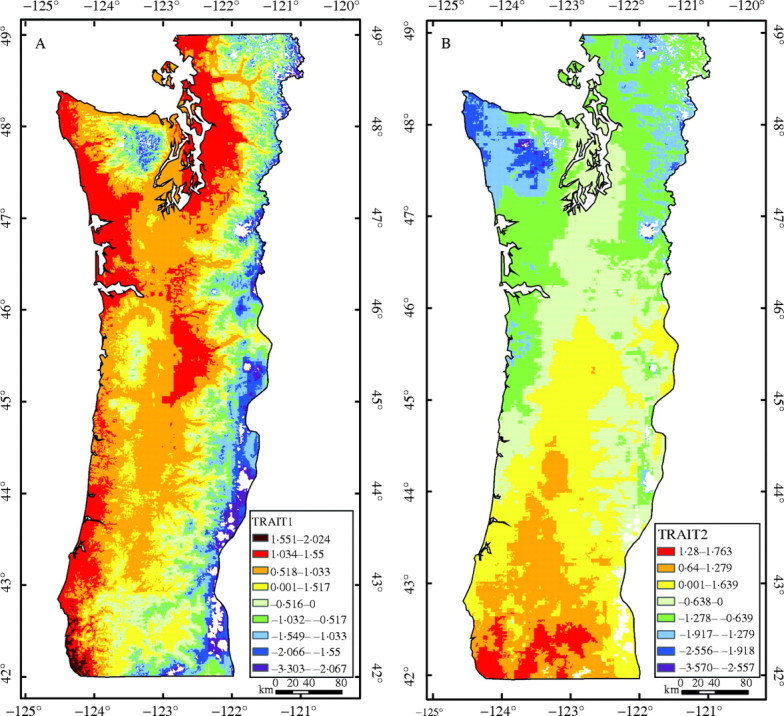
Geographical variation in (A) the first and (B) the second canonical variables for traits (TRAIT1 and TRAIT2, respectively). Mean values are shown as the zero contour between yellow and light green. Contour intervals represent a 30 % level of risk of maladaptation from source movement.

Fig. 4.

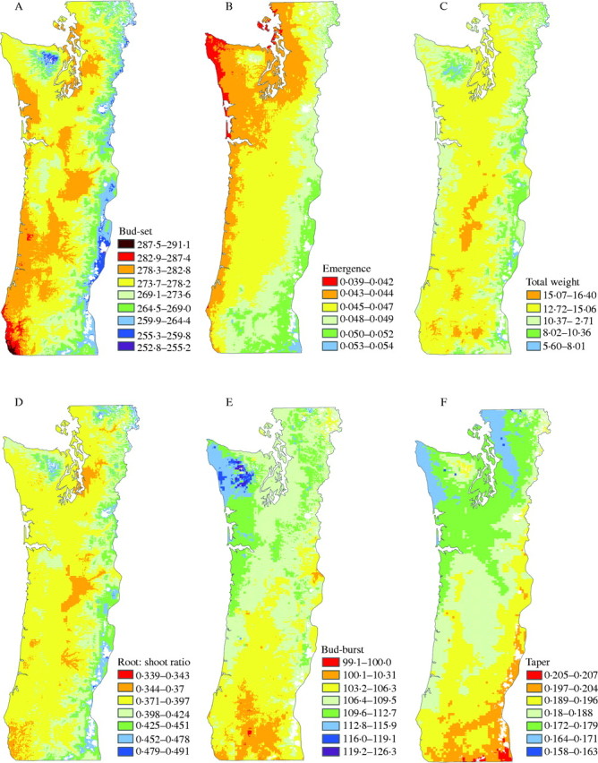
Geographical variation in traits of (A) first-year bud-set, (B) rate of emergence, (C) total weight, (D) root-to-shoot ratio, (E) second-year bud-burst and (F) taper. Mean values are shown as the contour between yellow and light green. Contour intervals represent a 30 % level of risk of maladaptation from source movement.

Maps of TRAIT1 and TRAIT2 were overlaid to visualize better areas of similar genetic types when considering both traits. Each trait was divided into three regions of low, medium and high values with the medium values consisting of the contour intervals immediately above and below the mean (i.e. the zero contour between the yellow and light green areas in Fig. 3), and the high and low values consisting of the contour intervals above and below the medium values. The resulting map clearly indicates that both elevation and latitude should be considered when trying to stratify the region into areas of similar genetic types (Fig. 5). High values for TRAIT1 (warm colours of red, orange and yellow) are all at the lower elevations, medium values (green colours) are all at middle elevations and low values (blue and purple colours) are all at high elevations. Within each elevation band, a latitudinal gradient exists from south to north corresponding to decreasing values for TRAIT2. This single map summarizes much of the variation in traits measured in the seedling common garden study.

Fig. 5.

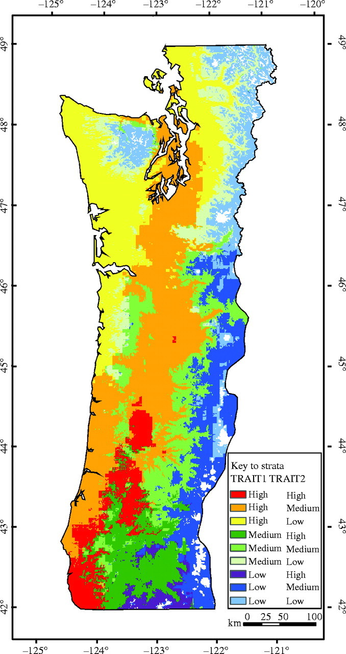
Map of areas of similar genetic types derived from overlaying the first and second canonical variables for traits.

Maps of residuals from the regression models indicate that sources from the eastside Washington Cascades differ considerably from the rest of the region in their relationship to the environment (Fig. 6). Seed sources on the eastside are much less vigorous (lower values of TRAIT1) and burst bud earlier (higher values of TRAIT2) than would be expected from the model developed for the rest of the region. For that reason, models and maps presented above were developed excluding sources from the eastside Washington Cascades (although the maps and models do not differ substantially whether or not they are included, largely because they represent a small portion of the total number of sources). For the rest of the region, the maps of residuals from the models do not indicate any large areas with large deviations from the overall models, but do indicate local areas that are more or less vigorous than expected or burst bud earlier or later than expected.

Fig. 6.

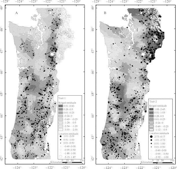
Maps of residuals from the model developed for (A) first and (B) second canonical variables for traits as a function of the environment. The magnitude and sign of the residual are indicated by the relative size of the open (positive) or closed (negative) circle for individual source locations. A kriging function in ARC/INFO was used to interpolate between source locations.

Discontinuous variation between west- and eastside Washington Cascades

The large difference in values for TRAIT1 between the west- and eastside Washington Cascades seen in the map of residuals from the model (Fig. 6) is also evident in graphs of TRAIT1 versus individual geographical or climatic variables. For a given elevation or December minimum temperature, sources from the eastern side of the Washington Cascades are much smaller and set bud earlier (lower values of TRAIT1) than sources from the western side of the Washington Cascades north of 46·5° latitude (Fig. 7A, B). This contrast between the east and west sides of the Cascades is not evident further south in Oregon; values of TRAIT1 largely overlap (Fig. 7C). The relationship between TRAIT1 and temperature within regions is similar on both sides of the Cascades (i.e. decreasing vigour with decreasing temperature or increasing elevation); however, the correlation is much weaker (or near zero for correlations with date of last spring frost or first fall frost) within the eastside Washington Cascades than in the westside Cascades or eastside Oregon Cascades (Table 9). Interestingly, the relation between precipitation and TRAIT1 differs between the eastside Washington Cascades and the other regions; within the eastside Washington Cascades, more vigorous sources come from areas of higher precipitation, whereas in the other regions, the correlations are either weak or, in the case of eastside Oregon sources, moderately negative.

Fig. 7.

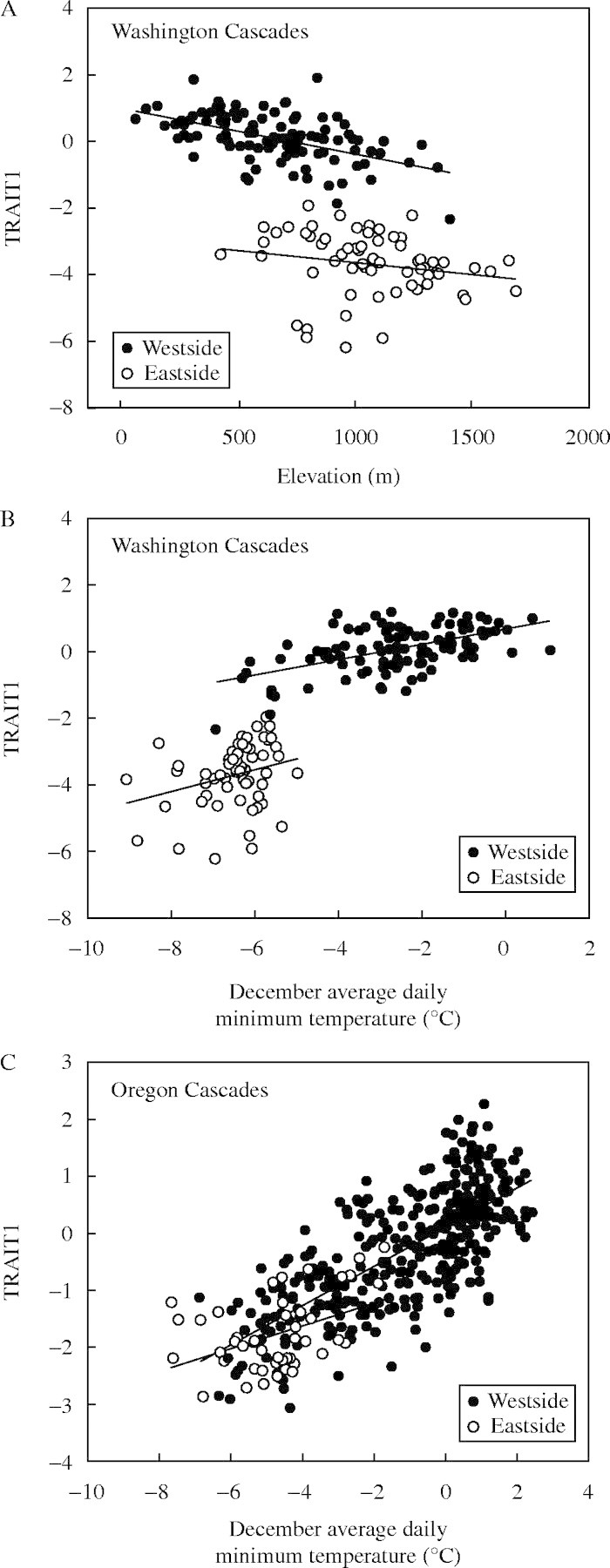
The first canonical correlation for traits (TRAIT1) as related to elevation and December average daily minimum temperature for sources on the eastside and westside Washington and Oregon Cascades.

Table 9.

Correlations between TRAIT1 and temperature and precipitation variables within regions

Environmental variable*	Eastside Washington Cascades†	Westside Washington Cascades‡	Eastside Oregon Cascades§	Westside Oregon Cascades¶
ELEV	−0·21	−0·52	−0·66	−0·74
DECMNT	0·28	0·51	0·40	0·72
SPRFRST	0·16	−0·45	−0·47	−0·69
FALLFRST	−0·06	0·45	0·45	0·69
ANNPRE	0·45	−0·11	−0·07	0·04
WINPRE	0·48	−0·15	0·03	−0·05
SUMPRE	0·37	−0·01	−0·35	−0·04
JULARID	0·35	−0·16	−0·55	−0·20

^*Key to environmental variables: ELEV = elevation, DECMNT = December average daily minimum temperature, SPRFRST = date of first spring frost, FALLFRST = date of last autumn frost, ANNPRE = total annual precipitation, WINPRE = total precipitation from December through February, SUMPRE = total precipitation from June through August, JULARID = ratio of July precipitation to July average temperature plus 10.

^†Correlations equal to or greater than 0·25 are significantly different from zero at P = 0·05.

^‡Correlations equal to or greater than 0·19 are significantly different from zero at P = 0·05.

^§Correlations equal to or greater than 0·27 are significantly different from zero at P = 0·05.

^¶Correlations equal to or greater than 0·10 are significantly different from zero at P = 0·05.

DISCUSSION

Maps generated using CCA and GIS allow easy visualization of a complex array of traits as related to environments. This methodology is particularly valuable in mountainous areas such as the Pacific Northwest with its complex topography and associated climates. CCA effectively reduces the number of traits from many to a few uncorrelated composite traits that explain much of the variation among traits and among locations (Table 3). These composite traits can be mapped using algebraic functions in GIS (Fig. 3). In this study, as few as two composite traits explain much of the variation among traits (45 % in the first two canonical variables, with each successive canonical variable explaining 13 % or less), and these two composite traits explain much of the variation among locations (68 and 50 %, with successive canonical variables explaining 11 % or less). The two composite traits show two distinct patterns of geographical variation, with variation in TRAIT1 showing an east–west cline associated with elevation and temperature, and variation in TRAIT2 showing a north–south cline associated with latitude and summer drought. The association of TRAIT1 with elevation is evident in the patterns of major drainages in the Cascades (Fig. 3). The visualization may be further simplified into a single two-dimensional map of overlaid traits (Fig. 5) when the number of uncorrelated traits explaining much of the variation is only two (or, in the case of three traits, a less easily visualized three-dimensional map may be created).

Temperature appears to be of overriding importance to the adaptation of Douglas fir to Pacific Northwest environments. TRAIT1 accounts for much of the variation among individual traits and is strongly related to the environments of source locations (the proportion of variance explained by traits and environments is 20 %; Table 3). The environmental variables with the highest correlations with TRAIT1 are temperature variables, particularly minimum temperatures in the winter months and dates of first spring and last autumn frost (Tables 6 and 7). Low temperatures appear to have resulted in natural selection for traits of earlier bud-set, presumably to avoid autumn frosts, and faster emergence, presumably to promote seedling establishment as soon as conditions are favourable in the spring. Higher temperatures, by contrast, appear to have resulted in natural selection for traits of increased growth and greater partitioning to shoots versus roots, presumably to promote competitive ability.

Of lesser importance to the adaptation of Douglas fir in the Pacific Northwest are environmental variables associated with summer drought. TRAIT2 accounts for less variation among individual traits and is less strongly related to the environments of source locations compared with TRAIT1 (the proportion of variance explained by traits and environments is 7 %; Table 3). TRAIT 2, and the component traits of bud-burst and taper, is most strongly correlated with precipitation and maximum temperature in the summer months (and aridity, a ratio of the two; Tables 6 and 7).Selection for earlier bud-burst may be hypothesized to be a mechanism to ensure sufficient early growth before drought becomes limiting. The correlation of bud-burst with latitude corresponds to a latitudinal trend in summer drought in the Pacific Northwest (r = 0·56 between latitude and summer precipitation). South-western Oregon is much warmer and drier in the summer than north-western Washington, particularly on the east side of the Coast Range and Siskiyou Mountains. Early bud-burst is commonly associated with trees from colder climates, probably as a result of either low chilling requirements, low heat sum requirements, or both (Morgenstern, 1996; Aitken and Hannerz, 2001; Howe et al., 2003). In our study, however, correlations of bud-burst with elevation or cold-season temperature variables are near zero (Table 7), and the strength of the relation is not improved by a using quadratic instead of a linear model (e.g. R² = 0·03 between bud-burst and elevation). Our individual-trait model did indicate some areas of early bud-burst in the higher elevations of the Cascades (Fig. 4E), and deviations from the model for TRAIT2 indicate areas where TRAIT2 was actually higher than predicted (i.e. earlier bud-burst) from the model in the North Cascades and on the eastside Washington Cascades (an area not included in the model development; Fig. 6B). However, the map of deviations from the model also indicates that bud-burst may actually be even earlier than predicted for some dry areas in Oregon. Others have found a similar relation between bud-burst and moisture deficit, July precipitation or latitude in Douglas fir, and have suggested natural selection of early bud-burst for drought avoidance (Campbell and Sugano, 1979; White et al., 1979).

Taper is also correlated with summer drought and latitude, but unlike bud-burst, shows some correlation with elevation (Table 7). Partitioning to diameter versus height may be related to drought tolerance, to light interception or to average stand density (i.e. number of trees per hectare). Trees that partition more to diameter versus height may have greater drought tolerances owing to lower crown volumes and transpiration. Trees that partition more to height may be better able to intercept light coming from lower on the horizon at higher latitudes, or might have higher competitive abilities in dense stands such as at the highly productive, wet-summer, low-elevation sites in Washington.

The patterns of variation and associations with environmental variables from this study generally match those found in previous studies of Douglas fir, and, to some extent, other species. Campbell (1986) and Campbell and Sugano (1993) studied geographical genetic variation in Douglas fir in south-western Oregon below about 43°N. Both studies considered traits of growth and bud phenology. Using principal component analysis to reduce the number of traits, the first principal component in both studies was analogous to the first canonical variable for traits in the current study, essentially vigour (faster growth and later bud-set), and the second principal component was analogous to the second canonical variable for traits, largely associated with bud-burst. Thus, the interrelations among traits were similar in all three studies. All three studies also accounted for similar amounts of variation in the relation between traits and environments: 66–68 % in the first component trait and 38–50 % of the variation in the second component trait. Campbell (1986) studied the area in the eastern half of south-western Oregon below 43°N. The pattern of variation in the first principal component generally follows a NW–SE cline (high to low vigour), which corresponds to the pattern found in this study (Figs 3A and 4A, C). The pattern of variation in the second principal component generally follows a west–east cline (early to late bud-burst), which also corresponds to the pattern found in this study (Figs 3B and 4E). Campbell and Sugano (1993) studied the area of the western half below 43°N. They found a cline in the first principal component from areas of high vigour in the south-west along the coast to low vigour in the north-west of the study area, again corresponding to patterns found in this study (Fig. 3A). The cline in the second principal component, however, differed from that found in this study. Bud-burst was later in the south-west corner of their study area, near the coast and the border with California, whereas bud-burst was somewhat earlier in that area in the current study (Figs 3B and 4E). The patterns of variation in both vigour and bud-burst were attributed to the effects of both drought and cold as determined by elevation, distance from the ocean and aspect. Distinguishing between effects of drought and cold is difficult because temperature or elevation is largely correlated with precipitation within the study areas in south-western Oregon; December minimum temperature and precipitation are uncorrelated in our study (r = 0·00). We conclude, based on sampling over a larger area, that drought is not associated with vigour, that cold is not associated with bud-burst, and that aspect, slope and sun-exposure are not associated with either trait. Nevertheless, the possibility exists that genecological relations are somewhat different in south-western Oregon, particularly in mountainous areas near the ocean, compared with other areas in western Oregon and Washington (Sorensen, 1983).

Genetic clines may occur over relatively short distances. Campbell (1979) considered variation within a single 6100-ha watershed in the central Oregon Cascades and found that the relation between traits and environment was of a similar magnitude to this study and the two studies from south-western Oregon (the regression of the principal component associated with growth and bud-set with physiographical variables accounted for 68 % of the variation, and the regression of the principal component associated with bud-burst with physiographical variables accounted for 50 % of the variation). Although the study area was small, the elevational range was large within the watershed (1100 m). As with other studies, vigour was strongly related to elevation, but unlike the current study, aspect had an effect. Bud-burst was not associated with elevation.

Campbell and Sorensen (1978) evaluated genetic variation as related to elevation, latitude and distance from the ocean in roughly the same area as the current study, but with only 40 locations sampled. As with the current study, seedling size and bud-set were associated with elevation, and bud-burst was associated with latitude. The relation between seedling size and elevation was stronger in the Cascades than in the Coast Range. They conclude that the risk of moving populations is greater in an east–west direction than north–south, although the risk was greater for north–south transfers in the Coast Range than the Cascades, that the risk increased as elevation of populations increased, and that the risk was less for elevational transfers in the Coast Range.

Results from studies of the interior variety of Douglas fir are similar to those discussed above. Seedling size, bud-set and autumn cold hardiness are most strongly related to elevation and the length of the growing season (Rehfeldt, 1979, 1982, 1983, 1989). Unlike in studies of the coastal variety, however, rates of genetic change are greater at lower elevations than at higher elevations; at elevations below 1000 m, populations separated by 240 m are genetically distinct, but near 1500 m, populations must be separated by 350 m to be distinct. These values are similar to the overall value in our study of 356 m for changes in elevation that correspond to a 30 % risk of seed movement (assuming a linear relation), which also correspond to general elevational transfer guidelines recommended for current seed zones for Douglas fir in Oregon and Washington (Randall, 1996; Randall and Berrang, 2002).

Despite considerable population variation that is strongly related to the environments of source locations, considerable genetic variation exists within Douglas fir populations. Thus, progress from selection within populations in tree improvement programmes is readily available. Nevertheless, breeding programmes should pay particular attention to maintaining geographical genetic structure, particularly with respect to bud-burst, bud-set and emergence rates, which all have high components of location variance and strong correlations with environments, indicating that they may be of particular adaptive importance. Reforestation and tree improvement programmes use breeding zones and seed zones to control the deployment of genetic material to appropriate sites to ensure adapted planting stock. Douglas fir zones are relatively restrictive in Oregon and Washington. Most seed zones have a long north–south orientation, but usually do not exceed much more than a degree in latitude, and are generally restricted to 300 m or less in elevation range (Randall, 1996; Randall and Berang, 2002). Breeding zones are generally larger in latitude, but are generally restricted to lower elevation sites. Thus, seed and breeding zones are roughly similar in size and orientation to the homogeneous genetic regions derived in this study (Fig. 5). The predominant traits of interest in tree improvement programmes are growth traits, which appear to have more room for selection (higher within-population variation) and are less correlated with environments than are phenological traits. Appropriate zones for growth traits would be somewhat larger than zones for phenological traits.

The maps of genetic variation indicate recurrence of similar populations across large geographical distances in areas that might be quite dissimilar from one another (Figs 3 and 5). For example, areas in the Coast Range appear to have Douglas fir populations that are genetically similar to those in areas in the Cascades, and areas in the Puget Sound appear to have populations that are genetically similar to those in areas on the central Oregon Coast Range. We caution, however, against moving populations such long distances. Although several traits important to adaptation were considered in this study, other traits important to adaptation were not evaluated. For example, traits of resistance or tolerance to disease and insects were not considered, and movements between coastal and inland sites may have implications for tolerance to Swiss needle cast (Johnson, 2002).

The large differences in growth and bud-set between populations west and east of the Cascade watershed in Washington is quite striking (Figs 6 and 7). The sharp break occurs despite a generally continuous distribution of the species, and the potential for unrestricted gene flow from wind pollination. We hypothesize that populations west of the watershed are of the coastal variety, menziesii, whereas populations east of the watershed are of the interior variety, glauca. Interior Douglas fir is slower growing, sets bud earlier and is more frost hardy than the coastal variety (Haddock et al., 1967; Rehfeldt, 1977; Sorensen, 1979; Hermann and Lavender, 1990). The distribution of Douglas fir is continuous across much of British Columbia, and the division between varieties is commonly considered to be at the crest of the British Columbia Coast Range with a zone of transition to the east (von Rudloff, 1973; Zavarin and Snajberk, 1973; Hermann and Lavender, 1990). Further south in Oregon, however, the west–east distribution is not continuous, and Little (1971) puts the division at the eastern edge of the Cascades. In contrast to data from the Oregon Cascades, our results suggest that the division is at the crest of the Cascades in Washington with a sharp transition zone. Li and Adams (1989) also found a sharp transition zone in Washington (and in British Columbia) in allozyme variation, although the number of samples was limited.

The sharp transition zone suggests that contact between the varieties is relatively recent. Following the Wisconsin glaciation (20 000 to 15 000 years BP, before present), Douglas fir appears to have spread north rapidly from glacial-age populations located in south-western Washington or western Oregon in the west, and from populations in the southern Rocky Mountains and Great Basin in the east (Tsukada, 1982; Wells, 1983; Critchfield, 1984; Hermann, 1985; Schnabel et al., 1993; Worona and Whitlock, 1995). Tsukada (1982) estimates the time of contact between the coastal and interior varieties as 7000 years BP based on the timing of the presence of pollen at a site in north-east Washington. The paleoecological record does not, however, give any clues as to the exact source area, timing and direction of the post-glacial migration of Douglas fir into the eastern Washington Cascades. Douglas fir did not appear to be abundant on the eastern side of the Oregon Cascades until about 4000 years ago (Whitlock and Bartlein, 1997), and modern forest species assemblages do not appear to have come into existence until about 2000–4000 years ago (Worona and Whitlock, 1995). We hypothesize that the interior variety of Douglas fir migrated south along the eastside Washington Cascades, and that contact at the crest of the Cascades has been within the last few thousand years. Varietal differences in flower phenology may also be hypothesized to have limited introgression between the two varieties at the zone of contact.

We did not find a sharp transition zone in the Oregon Cascades; the transition zone in Oregon appeared to be east of the Cascades and our sample area. Sorensen (1979) found a gradual transitional zone for adaptive traits between varieties in central Oregon that extended from the watershed of the Cascades east into the Blue Mountains, despite a narrow break of about 50 km in the distribution of the species that is commonly used to demarcate the varieties. A study of the same transect using presumably neutral RAPD markers showed a distinct boundary between varieties coinciding with the break in the distribution (Aagaard et al., 1995), which agrees with results from allozymes (Li and Adams, 1989) and terpene composition (Zavarin and Snajberk, 1973). In contrast to Douglas fir of the Washington Cascades, those of the eastside Oregon Cascades shares a genetic affinity with the coastal variety, and probably migrated from glacial-age populations on the westside.

One possibility is that the decreased growth and earlier bud-set in the Washington transition may be an adaptation to higher drought on the eastside, but this is not consistent with the finding that seedlings from the eastside are also smaller and set bud earlier for a given value of precipitation or July aridity. Seedlings from the eastside Washington Cascades are simply less vigorous, consistent with the idea that they are of the interior variety. Estimates of pollen- and seed-mediated gene flow from neutral DNA markers could potentially shed light on the presence and nature of barriers to gene flow across this narrow transition zone, as well as provide evidence for or against the hypothesis of varietal differences.

Adaptation of Douglas fir populations to their environments appears to be largely a consequence of trade-offs between selection for traits to avoid exposure to cold and traits that confer high vigour in mild environments. Winter temperatures are of greatest importance to population differentiation. Selection for drought avoidance by early bud-burst also appears to have resulted in population differentiation. An important unanswered question arising from this work is: what specific genetic and epigenetic phenomena are responsible for geographical variation observed in adaptive traits? To address this fundamental question, parents from this study are currently being genotyped at candidate genes presumably involved in cold hardiness and drought tolerance. Associations between DNA-level polymorphism and traits measured in this study should provide a first step to elucidating the genes or pathways responsible for adaptive variation in Douglas fir (Neale and Savolainen, 2004).

LITERATURE CITED

- Aagaard JE, Vollmer SS, Sorensen FC, Strauss SH. 1995. Mitochondrial DNA products among RAPD profiles are frequent and strongly differentiated between races of Douglas fir. Molecular Ecology 4: 441–447. [DOI] [PubMed] [Google Scholar]
- Aitken SN, Hannerz M. 2001. Genecology and gene resource management strategies for conifer cold hardiness. In: Bigras FJ, Columbo SJ, eds. Conifer cold hardiness. Dordrecht: Kluwer Academic Publishers, 25–53. [Google Scholar]
- Campbell RK. 1979. Genecology of Douglas fir in a watershed in the Oregon Cascades. Ecology 60: 1036–1050. [Google Scholar]
- Campbell RK. 1986. Mapped genetic variation of Douglas fir to guide seed transfer in southwest Oregon. Silvae Genetica 35: 85–96. [Google Scholar]
- Campbell RK. 1992. Genotype*environment interaction: a case study for Douglas fir in western Oregon. Research Paper PNW-RP-455. Portland, OR: US Department of Agriculture, Forest Service, Pacific Northwest Research Station, 21 pp. [Google Scholar]
- Campbell RK, Sorensen FC. 1978. Effect of test environment on the expression of clines and on delimitation of seed zones in Douglas fir. Theoretical and Applied Genetics 51: 233–246. [DOI] [PubMed] [Google Scholar]
- Campbell RK, Sorensen FC. 1979. A new basis for characterizing germination. Journal of Seed Technology 4: 24–34. [Google Scholar]
- Campbell RK, Sugano AI. 1979. Genecology of bud-burst phenology in Douglas fir: response to flushing temperature and chilling. Botanical Gazette 140: 223–231. [Google Scholar]
- Campbell RK, Sugano AI. 1993. Genetic variation and seed zones of Douglas fir in the Siskiyou National Forest. Research Paper PNW-RP-461. Portland, OR: US Department of Agriculture, Forest Service, Pacific Northwest Research Station, 23 pp. [Google Scholar]
- Cooley WW, Lohnes PR. 1971.Multivariate data analysis. New York: John Wiley & Sons. [Google Scholar]
- Cressie NAC. 1991.Statistics for spatial data. New York: John Wiley & Sons. [Google Scholar]
- Critchfield WB. 1984. Impact of the Pleistocene on the genetic structure of North American conifers. In: Lanner RM, ed. Proceedings of 8th North American Forest Biology Workshop. Logan, UT: Utah State University, 70–118. [Google Scholar]
- Daly C, Neilson RP, Phillips DL. 1994. A statistical–topographic model for mapping climatological precipitation over mountainous terrain. Journal of Applied Meteorology 33: 140–158. [Google Scholar]
- Endler JA. 1986.Natural selection in the wild. Princeton, NJ: Princeton University Press. [Google Scholar]
- Haddock PG, Walters J, Kozak A. 1967. Growth of coastal and interior provenances of Douglas fir (Pseudotsuga menziesii (Mirb.) Franco) at Vancouver and Haney in British Columbia. Faculty of Forestry Research Paper No. 79. Vancouver: University of British Columbia. [Google Scholar]
- Hermann RK. 1985. The genus Pseudotsuga: ancestral history and past distribution. Special Publication 2b. Corvallis, OR: Forest Research Laboratory, Oregon State University. [Google Scholar]
- Hermann RK, Lavender DP. 1968. Early growth of Douglas fir from various altitudes and aspects in southern Oregon. Silva Genetica 17: 143–151. [Google Scholar]
- Hermann RK, Lavender DP. 1990.Pseudotsuga menziesii (Mirb.) Franco Douglas fir. In: Burnes RM, Honkala BH, eds. Silvics of North America. Volume 1. Conifers. Agriculture Handbook 654. Washington, DC: US Department of Agriculture, Forest Service, 527–540. [Google Scholar]
- Heslop-Harrison J. 1964. Forty years of genecology. In: Cragg JB, ed. Advances in ecological research. Vol. Two. New York: Academic Press, 159–247. [Google Scholar]
- Howe GT, Aitken SN, Neale DB, Jermstad KD, Wheeler NC, Chen THH. 2003. From genotype to phenotype: unraveling the complexities of cold adaptation in forest trees. Canadian Journal of Botany 81: 1247–1266. [Google Scholar]
- Griffin AR. 1978. Geographic variation in Douglas fir from the coastal ranges of California. II. Predictive value of a regression model for seedling growth variation. Silvae Genetica 27: 96–101. [Google Scholar]
- Griffin AR, Ching KK. 1977. Geographic variation in Douglas fir from the coastal ranges of California. I. Seed, seedling growth and hardiness characteristics. Silvae Genetica 26: 149–157. [Google Scholar]
- Johnson GR. 1997. Site-to-site genetic correlations and their implications on breeding zone size and optimum number of progeny test sites for coastal Douglas fir. Silvae Genetica 46: 280–285. [Google Scholar]
- Johnson GR. 2002. Genetic variation in tolerance of Douglas fir to Swiss needle cast as assessed by symptom expression. Silvae Genetica 51: 80–86. [Google Scholar]
- Li P, Adams WT. 1989. Range-wide patterns of allozyme variation in Douglas fir (Pseudotsuga menziesii). Canadian Journal of Forest Research 19: 149–161. [Google Scholar]
- Little EL. 1971.Atlas of United States trees. Volume 1. Conifers and important hardwoods. Miscellaneous Publication No. 1146. Washington, DC: US. Department of Agriculture, Forest Service. [Google Scholar]
- Mardia KV, Kent JT, Bibby JM. 1979.Multivariate analysis. London: Academic Press. [Google Scholar]
- Morgenstern EK. 1996.Geographic variation in forest trees. Vancouver: UBC Press. [Google Scholar]
- Neale DB, Savolainen O. 2004. Association genetics of complex traits in conifers. Trends in Plant Sciences 9: 325–330. [DOI] [PubMed] [Google Scholar]
- Neter J, Wasserman W. 1974.Applied linear statistical models. Homewood, IL: Richard D. Irwin, Inc. [Google Scholar]
- Randall WK. 1996.Forest tree seed zones for western Oregon. Salem, OR: State of Oregon Department of Forestry. [Google Scholar]
- Randall WK, Berrang P. 2002.Washington tree seed transfer zones. Olympia, WA: Washington State Department of Natural Resources. [Google Scholar]
- Rehfeldt GE. 1977. Growth and cold hardiness of intervarietal hybrids of Douglas fir. Theoretical and Applied Genetics 50: 3–15. [DOI] [PubMed] [Google Scholar]
- Rehfeldt GE. 1979. Ecological adaptations in Douglas fir (Pseudotsuga menziesii var. glauca) populations. I. North Idaho and north-east Washington. Heredity 43: 383–397. [Google Scholar]
- Rehfeldt GE. 1982. Ecological adaptations in Douglas fir populations. II. Western Montana. Research Paper INT-295. Ogden, UT: US Department of Agriculture, Forest Service, Intermountain Forest and Range Experiment Station, 8 pp. [Google Scholar]
- Rehfeldt GE. 1983. Ecological adaptations in Douglas fir (Pseudotsuga menziesii var. glauca) populations. III. Central Idaho. Canadian Journal of Forest Research 13: 626–632. [Google Scholar]
- Rehfeldt GE. 1989. Ecological adaptations in Douglas fir (Pseudotsuga menziesii var. glauca): a synthesis. Forest Ecology and Management 28: 203–215. [Google Scholar]
- Rehfeldt GE. 1994. Evolutionary genetics, the biological species, and the ecology of the Interior cedar–hemlock forests. In: Proceedings of Interior cedar–hemlock–white pine forests: ecology and management. Pullman, WA: Washington State University, 91–100. [Google Scholar]
- von Rudloff E. 1973. Chemosytematic studies in the genus Pseudotsuga III. Population differences in British Columbia as determined by volatile leaf oil analysis. Canadian Journal of Forest Research 3: 443–452. [Google Scholar]
- SAS Institute Inc. 1999.SAS/STAT® user's guide, Version 8. Cary, NC: SAS Institute Inc. [Google Scholar]
- Schnabel A, Hamrick JL, Wells PV. 1993. Influence of Quaternary history on the population genetic structure of Douglas fir (Pseudotsuga menziesii) in the Great Basin. Canadian Journal of Forest Research 23: 1900–1906. [Google Scholar]
- Silen RR, Mandel NL. 1993. Clinal genetic growth variation within two Douglas fir breeding zones. Journal of Forestry 81: 216–220. [Google Scholar]
- Sorensen FC. 1979. Provenance variation in Pseudotsuga menziesii seedlings from the var. menziesii—var. glauca transition zone in Oregon. Silvae Genetica 28: 37–119. [Google Scholar]
- Sorensen FC. 1983. Geographic variation in seedling Douglas fir (Pseudotsuga menziesii) from the western Siskiyou Mountains of Oregon. Ecology 34: 696–702. [Google Scholar]
- Sorensen FC. 1992. Genetic variation and seed transfer guidelines for lodgepole pine in central Oregon. Research Paper PNW-RP-453. Portland, OR: US Department of Agriculture, Forest Service, Pacific Northwest Research Station, 30 pp. [Google Scholar]
- Stonecypher RW, Piesch RF, Helland GG, Chapman JG, Reno HJ. 1996. Results from genetic tests of selected parents of Douglas fir (Pseudotsuga menziesii (Mirb.) Franco) in an applied tree improvement program. Forest Science 42: Monograph 32: 1–35. [Google Scholar]
- Tsukada M. 1982.Psuedotsuga menziesii (Mirb.) Franco: its pollen dispersal and late Quaternary history in the Pacific Northwest. Japanese Journal of Ecology 32: 159–187. [Google Scholar]
- Wartenberg D. 1985. Canonical trend surface analysis: a method for describing geographic patterns. Systematic Zoology 34: 259–279. [Google Scholar]
- Wells PV. 1983. Paleobiogeography of montane islands in the Great Basin since the last glaciopluvial. Ecological Monographs 53: 341–382. [Google Scholar]
- White TL, Ching KK. 1985. Provenance study of Douglas fir in the Pacific Northwest region. IV. Field performance at age 25 years. Silvae Genetica 34: 84–90. [Google Scholar]
- White TL, Hodges GR. 1989.Predicting breeding values with applications in forest tree improvement. Dordrecht: Kluwer Academic Publishers. [Google Scholar]
- White TL, Ching KK, Walters J. 1979. Effects of provenance, years, and planting location on bud burst of Douglas fir. Forest Science 25: 161–167. [Google Scholar]
- Whitlock C, Bartlein PJ. 1997. Vegetation and climate change in northwest America during the past 125 kyr. Nature 388: 57–61. [Google Scholar]
- Worona MA, Whitlock C. 1995. Late Quaternary vegetation and climate history near Little Lake, central Coast Range, Oregon. Geological Society of America Bulletin 107: 867–876. [Google Scholar]
- Zavarin E, Snajberk K. 1973. Geographical variability of monoterpenes from cortex of Pseudotsuga menziesii Pure and Applied Chemistry 34: 411–434. [Google Scholar]