Specific Leaf Area and Dry Matter Content Estimate Thickness in Laminar Leaves

Abstract

• Background and Aims Leaf thickness plays an important role in leaf and plant functioning, and relates to a species' strategy of resource acquisition and use. As such, it has been widely used for screening purposes in crop science and community ecology. However, since its measurement is not straightforward, a number of estimates have been proposed. Here, the validity of the (SLA × LDMC)⁻¹ product is tested to estimate leaf thickness, where SLA is the specific leaf area (leaf area/dry mass) and LDMC is the leaf dry matter content (leaf dry mass/fresh mass). SLA and LDMC are two leaf traits that are both more easily measurable and often reported in the literature.

• Methods The relationship between leaf thickness (LT) and (SLA × LDMC)⁻¹ was tested in two analyses of covariance using 11 datasets (three original and eight published) for a total number of 1039 data points, corresponding to a wide range of growth forms growing in contrasted environments in four continents.

• Key Results and Conclusions The overall slope and intercept of the relationship were not significantly different from one and zero, respectively, and the residual standard error was 0·11. Only two of the eight datasets displayed a significant difference in the intercepts, and the only significant difference among the most represented growth forms was for trees. LT can therefore be estimated by (SLA × LDMC)⁻¹, allowing leaf thickness to be derived from easily and widely measured leaf traits.

INTRODUCTION

Leaf thickness (LT) plays an important role in leaf and plant functioning and is related to species' strategies of resource acquisition and use. The amount of light absorbed by a leaf, and the diffusion pathway of CO₂ through its tissues depend, at least partially, on its thickness (Givnish, 1979; Agusti et al., 1994; Syvertsen et al., 1995). Negative relationships between LT and photosynthetic (Enriquez et al., 1996; Garnier et al., 1999) and growth (Poorter, 1990; Nielsen et al., 1996) rates have been observed, and thicker leaves have sometimes been associated with increased longevity and construction costs (Mediavilla et al., 2001; Westoby et al., 2002). Leaf thickness has therefore often been used as a tool to screen species and/or cultivars for productivity (e.g. Dornhoff and Shibles, 1976; White and Montes-R, 2005) or ecological performance (Witkowski et al., 1992; Díaz et al., 2004).

The determination of leaf thickness is not straightforward, however. The wide variation in leaf morphology (e.g. presence of specialized structures on leaf surface like hairs and spines or protruding veins), the differences in thickness within individual leaves, and the fact that thickness is a relatively small dimension (sometimes <100 µm in terrestrial plants) make LT difficult and time consuming to measure accurately. Leaf thickness has therefore often been estimated, and a number of surrogates have been proposed and used (see White and Montes-R, 2005). One such estimate is the ratio of leaf fresh mass to surface area (e.g. Atkin et al., 1996; Wright and Westoby, 2002), but as far as is known, the validity of this approximation has not been formally tested (but see Sims et al., 1998; White and Montes-R, 2005). Building on Witkowski and Lamont (1991) and Roderick et al. (1999a), it is shown below that this ratio relates to two other, widely measured leaf traits: specific leaf area (SLA, the ratio of leaf area to leaf dry mass) and leaf dry matter content (LDMC, the ratio of leaf dry mass to saturated fresh mass = 1 – leaf water content). The aim of this paper is to demonstrate that LT can be safely deduced from these two traits, which are much easier to measure.

The mean thickness of a laminar leaf (LT) can be calculated as the ratio of its volume (V_L) to its projected area (A) (e.g. Roderick et al., 1999a): LT = V_L/A. Let ρ_F be the average density of the leaf [the leaf fresh mass (M_F) to volume (V_L) ratio], thickness can be expressed as: LT = (1/ρ_F)(M_F/A). Note that ρ is not the density of leaf tissues (tissue mass per tissue volume) because it includes the mass and volume of leaf water as well as the volume of intercellular spaces. Incorporating leaf dry mass (M_D) into this expression leads to:

Using the leaf fresh mass to surface area ratio or (SLA × LDMC)⁻¹ as estimates of LT suggests that leaf fresh mass is a good estimate of leaf volume (with the consequence that ρ_F ≈ 1), which has already been shown in a number of cases (Sims et al., 1998; Garnier et al., 1999). Here, the relationship between LT and (SLA × LDMC)⁻¹ will be tested further, using an extensive data set consisting of 1039 data points collected from three original and eight published studies covering widely differing geographical areas, species and growth forms.

MATERIALS AND METHODS

Original studies

Study sites

The three original experiments were conducted in sites with a Mediterranean climate. The first one [‘French Mediterranean old fields’, hereafter FR-Med; described in Aronson et al. (1998) and Garnier et al. (2004)] were located near Montpellier (France, 43°46′N, 3°42′E, 280 m a.s.l.). The second one [‘Garraf’, hereafter SP-Med; 41°18′N, 1°54′E, 300 m a.s.l.; see Lloret (1998) for details] was located near Barcelona (Spain) in the Garraf Natural Park. In these sites, the vegetation is typical of Mediterranean old-fields and shrublands (‘garrigue’) found on soil derived from a limestone substrate. The third site [Jonaskop', hereafter SA-Med; 33°58′S, 19°30′E, 450–1646 m a.s.l.; see Rutherford (1978) for details] was located at the limit of a South African nature reserve, in the Fynbos–Renosterveld–Karoo ecotone.

Species and harvests

In FR-Med, a total of 44 species were studied (data from the same species measured in different locations were considered as independent data points). Twenty-two of them were selected from Garnier et al. (2001a), and, adding to this set of species, two additional harvests were conducted in July 2001 (seven species) and May 2002 (15 species). In SP-Med and SA-Med, 46 species harvested in June 2001 and 46 species harvested in September 2002 were studied. At each site, species were selected from the most abundant ones (FR-Med, Garnier et al.; 2001a; SP-Med, F. Lloret and M. Vilà, unpubl. res.; SA-Med, G. F. Midgley, unpubl. res.). The species belong to more than 29 families (some species not yet identified in SA-Med) and span a very wide range of growth forms (see Tables 1 and 5). Species were classified according to their growth form (see Table 1); forbs include all herbaceous dicotyledonous species (including Fabaceae).

Table 1.

Characteristics of the studies from which data were taken

Study name	Reference	Country	No. of species	Growth forms	Device and rehydration procedure*
Original studies
FR-Med			France	44	Short-lived forbs (7)	Linear variable displacement transducer
				Long-lived forbs (5)	24 h in test tubes with deionized water in the dark at 4 °C
				Short-lived graminoids (2)
				Long-lived graminoids (9)
				Shrubs (17)
				Trees (4)
				Succulent (1)
SP-Med			Spain	46	Long-lived forbs (4)	Linear variable displacement transducer
				Long-lived graminoids (6)	24 h in test tubes with deionized water in the dark at 4 °C
				Shrubs (22)
				Trees (14)
				Succulent (1)
SA-Med			South Africa	46	Long-lived forbs (3)	Linear variable displacement transducer
				Long-lived graminoids (3)	24 h in test tubes with deionized water in the dark at 4 °C
				Shrubs (17)
				Trees (7)
				Not available (16)†
				Succulents (4)
Published studies
EU-1	Ryser and Urbas (2000)	Central Europe	27	Long-lived graminoids (27)	ID-C digimatic indicator (0·01 mm)
					One night rehydration
EU-2	Wilson et al. (1999)‡	Great Britain	632	Short-lived forbs (179)	Verdict analogue thickness gauge
				Long-lived forbs (331)	Hydrated over night in moist tissue paper in sealed polythene bags in a refrigerator (4 °C)
				Short-lived graminoids (10)
				Long-lived graminoids (70)
				Ferns (19)
				Shrubs (18)
				Tree (1)
				Others (4)
				Succulents (9)
AR-Cen	Vendramini et al. (2002)	Central Argentina	55	Short-lived forbs (3)	Cross-sectional observations under microscope
				Long-lived forbs (11)	No, but harvested after rainfall
				Trees (26)
				Short-lived graminoids (2)
				Long-lived graminoids (13)
				Succulents (22)
CA-Qué	Shipley (1995)	Canada	33	Short-lived forbs (8)	Dial gauge micrometer
				Long-lived forbs (21)	Plants, harvested with roots, immediately brought back to the lab and given free access to water; measurements done within 3 h after harvest.
				Graminoids (2)
				Shrubs (2)
AU-1	Cunningham et al. (1999)	Australia	37	Shrub (1)	Cross-sections and image analysis
				Trees (36)	(2) 10-min hydration
				Succulent (1)
AU-2	Roderick et al. (1999b)	Australia	26	Long-lived forbs (4)	Dial thickness gauge
				Shrubs (2)	Yes and no (no difference between the two)
				Trees (20)
AU-3	Wright (2001)	Australia	70	Shrubs (53)	Dial gauge micrometer
				Trees (17)	Overnight between sheets of damp paper towel at 4 °C
AU-4	Prior et al. (2003)	Australia	23	Trees (23)	Dial gauge micrometer
					Overnight between sheets of damp paper

For Tables 2–5 and Fig. 1, only laminar leaved species were considered (i.e. rolled and needle leaves were excluded); total species number is given in column 4 and detailed by growth forms in column 5. The number of succulent species used in Fig. 2 is added in column 5 (these species were not included in the calculation of total number of species shown in column 4).

^*Information about the ‘device’ which is the piece of equipment used to measure thickness is followed by the rehydration procedure of how leaves were rehydrated before the measurement of fresh mass.

^†These 16 taxa were not identified to the species level, and in the absence of unequivocal information, these were not assigned to a specific growth form.

^‡Aquatics were removed from the original data set because their particular leaf anatomy confounds predictions of density.

Measurement of leaf traits

For the three study sites, all material was collected from robust, well-grown plants. For herbaceous and small woody species, samples were taken from plants in full light; while for tall woody species, these were taken from the part of the plant lit by direct sunlight at the time of sampling. Six (SA-Med) or ten (FR-Med and SP-Med) replicate samples per species were used to calculate mean SLA and LDMC. After cutting from the plants, the samples (stem or twig segments bearing leaves) were wrapped in moist paper and conserved in a cool box until further processing. In the laboratory, they were rehydrated according to the standardized protocol described by Garnier et al. (2001b). After rehydration, the youngest fully expanded leaves free from herbivore or pathogen damage were chosen from each stem. The traits were measured for leaf blades only (petiole and/or rachis were removed). To determine the saturated fresh mass of leaves, they were immediately weighed. The projected area (one side of the leaf) was determined with an area meter (model MK2; Delta-T Devices, Cambridge, UK). From this, five (FR-Med and SP-Med) or six (SA-Med) replicate samples were used to determine LT with a linear variable displacement transducer (LVDT) (GDL case, models L2 and L5; IFELEC, T.N.C.), calibrated with metal strips of known thickness. Depending on the size of the individual leaves, LT was measured on five to ten points per leaf (blade), avoiding the mid-vein. Leaves were then oven-dried at 60 °C for at least 2 d, and their dry mass was determined. From these measurements, mean values of LDMC, SLA and LT were calculated.

Published studies

A literature survey was conducted to find studies where LT, SLA and LDMC had been measured simultaneously. SLA and LDMC were preferred to M_F and A since the latter are seldom available in the literature. Eight published studies conducted in different biomes and climate types were selected (Table 1), for a total of 964 plant species belonging to 120 families. The species were classified according to their growth form (see Table 1). Only studies in which traits were measured after some re-hydration prior to measurement were selected (Garnier et al., 2001b for discussion). The methods differed among studies (see Table 1). In particular, Vendramini et al. (2002) considered that collecting leaves in the morning immediately after rainfall insured their full hydration. LT was also measured with different pieces of equipment (Table 1).

In Roderick et al. (1999b), leaf traits were measured on shade and sun leaves for 13 species. Since the relationships between LT and (SLA × LDMC)⁻¹ for shade and sun leaves were not significantly different either in slopes (F = 0·019, n.s.) or intercepts (F = 0·958, n.s.) of the two regression lines, the two subsets were merged.

Due to theoretical considerations (see the Introduction), only species with laminar leaves were selected from these studies, i.e. species with rolled or needle leaves were excluded.

Statistical analysis

Statistical analyses were conducted in two ways, using a total of 1039 data points (Table 1). First, the data were analysed on the basis of the 11 data sets derived from the original and published studies described in Table 1; secondly, the data were grouped and analysed by growth form. Statistical analyses were conducted for the five growth forms represented by >100 data points, but means and standard errors are given for a total of seven growth forms (cf. Table 2).

Table 2.

Means and standard errors (s.e.) of traits and results of ANOVA (log-transformed values) by growth forms represented by more than 100 species (values in bold)

		LT		SLA			LDMC			ρF
Growth form	n	Mean	s.e.	Mean	s.e.	Mean	s.e.	Mean	s.e.
Ferns	19	232·9	22·6	17·4	1·3	281·3	13·2	1·11	0·10
Short-lived forbs	200	267·2a	11·7	26·2a	0·6	164·0a	3·5	1·12a	0·02
Long-lived forbs	379	254·3a	8·1	26·2a	0·5	190·6b	3·6	1·05b	0·01
Short-lived graminoids	14	163·4	16·5	24·0	2·1	292·8	23·7	1·02	0·07
Long-lived graminoids	129	229·1b	12·2	22·3b	0·9	304·5c	8·7	0·91c	0·03
Shrubs	132	429·1c	21·2	9·10c	0·6	383·5d	8·4	0·96d	0·02
Trees	148	416·0c	16·2	8·30c	0·4	414·7d	8·1	0·96d	0·02

Means with different letters are significantly different (Fisher LSD test; P < 0·05).

n, number of species; LT, leaf thickness (µm); SLA, specific leaf area (m² kg⁻¹); LDMC, leaf dry matter content (mg g⁻¹); ρ_F, leaf fresh density = (LT × SLA × LDMC)⁻¹.

All data were computed to obtain (SLA × LDMC)⁻¹ and leaf (fresh) density ρ_F (calculated as (LT × SLA × LDMC)⁻¹; see eqn 1). Mean trait values were computed for each growth form and the variation in mean trait values among the five most represented growth forms were evaluated by an analysis of variance (ANOVA). The Fisher LSD post-hoc test was used to test for growth form differences when the ANOVA was significant at the 5 % level of probability.

Equation 1 is considered as a linear model equation where LT is regressed on (SLA × LDMC)⁻¹ for each study. A logarithmic transformation was applied to the data in order to conform GLM residuals with GLM assumptions. After transformation, eqn 1 becomes: log(LT) = −log(ρ_F) + log[(SLA × LDMC)⁻¹] which holds exactly for a single leaf. Since leaf density (ρ_F) is the ratio of fresh mass to leaf volume, and since this fresh mass is primarily water (whose density is 1 g cm⁻³), it was hypothesised that ρ_F ≈ 1. Given the null hypothesis (H₀) , a regression of log(LT) on log[(SLA × LDMC)⁻¹] for a given data set (based on study or growth form) will have an intercept equal to 0. If the assumption of ρ_F ≈ 1 holds across the different data sets, geographical locations, species and growth forms, then there will be no significant difference in the intercepts between data sets. If there is no systematic deviation in either the higher or lower end of the LT range, then the overall slope will be one and there will be no significant difference in the slopes between data sets. Therefore two GLMs of covariance (ANCOVA) were fitted by regressing log(LT) as function of a class variable indicating (a) the study or (b) the growth form, log[(SLA × LDMC)⁻¹] as a covariate, and the interaction between the two. Significance was assessed at the 5 % level using F-tests based on type III sums of squares. Correlations between LT, SLA, LDMC, (SLA × LDMC)⁻¹ and ρ_F were tested using Pearson's correlation coefficients.

Although the analyses carried out here are formally valid for laminar leaves only, tests were also carried out to determine if some generalizations might be possible for succulent leaves, a type of non-laminar leaves that was well represented in some of the studies listed in Table 1.

RESULTS

Overview of data

Correlations between the three measured, log-transformed variables were all significant: SLA was strongly, negatively, correlated to LT and LDMC (r = −0·71 and −0·74, respectively), but LT and LDMC were only weakly correlated (r = 0·18). Whereas LT was significantly negatively correlated to ρ_F (r = −0·43), a very weak correlation coefficient (r = 0·07; P = 0·03) was found between (SLA × LDMC)⁻¹ and ρ_F. Table 2 shows the mean values and standard errors of LT, LDMC, SLA and ρ_F for each growth form. Each trait varied significantly among the five most represented growth forms (ANOVA, all P < 0·001; Table 2), but woody species appeared to form a homogeneous group since the mean values for the four traits did not differ significantly between shrubs and trees. Among the five growth forms, leaves of woody species were thicker and had a higher dry matter content, and a lower SLA, than forbs and graminoids. Forbs had thicker leaves and lower LDMC but significantly higher SLA than long-lived graminoids. LDMC seemed to better discriminate the growth forms since short- and long-lived forbs differed for mean LDMC values with higher dry matter content in long-lived forbs; LDMC of shrubs and trees were also marginally significantly different (P = 0·053). Leaf density on a fresh mass basis, calculated as (LT × SLA × LDMC)⁻¹, increased from long-lived graminoids to woody species, long-lived forbs, and short-lived forbs, respectively, but all values were close to 1.

Testing the model

For all studies, the log-linear relationship between LT and (SLA × LDMC)⁻¹ was highly significant (P < 0·001) and the percentage of variation in LT explained by (SLA × LDMC)⁻¹ varied from 50 to a maximum of 90 % (Table 3). Two studies (EU-2 and AR-Cen) showed an intercept that was significantly different from zero (Table 3 and Fig. 1A), indicating an overall mean leaf density different from one. The slopes of the different regression lines varied from 0·79 (AR-Cen) to 1·20 (EU-1). The only slope which differed significantly from 1 was for the EU-2 dataset (P < 0·001); for the AR-Cen and EU-1 datasets, the slopes were marginally significantly different from 1 (P = 0·059 and P = 0·082).

Table 3.

Linear regression coefficients associated with regression lines in Fig. 1

Study‡	Intercept (a)	Slope (b)	PH0: b=1	r2	n
Original studies
FR-Med	0·045 n.s.	1·001***	n.s.	0·69***	44
SA-Med	0·194 n.s.	0·956***	n.s.	0·78***	46
SP-Med	–0·106 n.s.	1·039***	n.s.	0·68***	46
Published studies
EU-1	–0·317 n.s.	1·197***	†	0·83***	27
EU-2	0·209***	0·905***	***	0·70***	632
AR-Cen	0·646*	0·789***	†	0·50***	55
CA-Qué	–0·116 n.s.	1·014***	n.s.	0·65***	33
AU-1	0·186 n.s.	0·939***	n.s.	0·60***	37
AU-2	0·314 n.s.	0·888***	n.s.	0·82***	26
AU-3	0·167 n.s.	0·937***	n.s.	0·82***	70
AU-4	0·278 n.s.	0·882***	n.s.	0·90***	23
All studies combined
	0·094* ± 0·082	0·963*** ± 0·034	n.s.	0·76***	1039

Linear regression coefficients and associated 95 % confidence intervals for all the studies (total). Regression for all studies is shown on Fig. 1C. Linear model: log(LT) = a + b log[(SLA × LDMC)⁻¹].

LT, measured leaf thickness (µm); SLA, specific leaf area (m² kg⁻¹); LDMC, leaf dry matter content (mg g⁻¹).

^***P < 0·001;

^**P < 0·01;

^*P < 0·050.

†: P < 0·100.;

n.s., not significant.

^‡See Table 1 for study names.

Fig. 1.

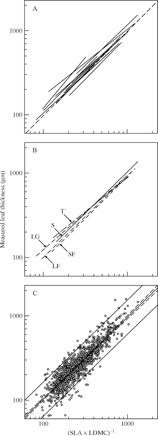
Linear regression relationships between measured leaf thickness (LT, μm) and the inverse of the product of specific leaf area (SLA, m² kg⁻¹) and leaf dry matter content (LDMC, mg g⁻¹). Note the logarithmic scales. (A) Regression lines of studies (each line represents one study); (B) regression lines of growth forms [each line represents one of the five most represented (n > 100) growth forms: SF, short-lived forbs (short-dashed line); LF, long-lived forbs (dashed-dotted line); LG, long-lived graminoids (medium-dashed line); S, shrubs (continuous line); T, trees (long-dashed line)]; (C) all data points (each point represents one species) except AR-Cen and GR-Grw, with general regression line (thick continuous line), confidence intervals (dashed lines) and prediction intervals (thin continuous lines). Log (LT) = 0·04 + 0·98 log [(SLA × LDMC)⁻¹]; r² = 0·79; n = 858; P < 0·001.

When data for all studies were pooled together, the linear relationship between LT and (SLA × LDMC)⁻¹ was highly significant (Table 3, n = 1039; P < 0·001; r = 0·87; Fig. 1). Further, no significant difference was detected between either the slopes (F_10,1039 = 1·23, P = 0·268; Table 4) or the intercepts (F_10,1039 = 1·55, P = 0·115) of the individual studies. If there were site differences then they were too small to be detected even though statistical power was strong (n = 1039). The overall intercept was only marginally significantly different from zero when all the studies were combined (F_1,1039 = 3·27, P = 0·071). This ANCOVA model explained 80 % of the total variance. The residual standard error was 0·112. The relationship appeared thus to be largely independent of geographical location of the species studied.

Table 4.

Analysis of covariance for all studies combined, for growth forms for which n > 100, and for growth forms for which n > 100 except AR-Cen

Source	Type III SS	d.f.	MS	F	P
All studies
Intercept	0·03	1	0·03	3·27	†
Study	0·16	10	0·02	1·55	n.s.
log[(SLA × LDMC)−1]	10·3	1	10·3	995	***
log[(SLA × LDMC)−1]× study	0·13	10	0·01	1·23	n.s.
Error	10·5	1017	0·01
Total	6136	1039
Growth forms
Intercept	0·18	1	0·18	16·90	***
Growth form	0·17	4	0·04	3·92	**
log[(SLA × LDMC)−1]	23·08	1	23·08	2145	***
log[(SLA × LDMC)−1]×     growth form	0·13	4	0·03	2·95	*
Error	10·52	978	0·01
Total	5823	988
Growth forms except AR-Cen
Intercept	0·08	1	0·08	9·59	***
Growth form	0·03	4	0·01	0·86	n.s.
log[(SLA × LDMC)−1]	19·24	1	19·24	2229	***
log[(SLA × LDMC)−1]×    growth form	0·02	4	0·01	0·65	n.s.
Error	7·98	925	0·01
Total	5457	935

General linear model: log(LT) = intercept + study + log[(SLA × LDMC)⁻¹] + log[(SLA × LDMC)⁻¹]× study.

LT, measured leaf thickness (µm), SLA, specific leaf area (m² kg⁻¹); LDMC, leaf dry matter content (mg g⁻¹). See also Fig. 1.

^***P < 0·001;

^**P < 0·01;

^*P < 0·050.

^†P < 0·100;

n.s., not significant.

When species were grouped by growth form, the log-linear relationship between LT and (SLA × LDMC)⁻¹ was highly significant (P < 0·001) for all growth forms (Table 5 and Fig. 1B). The percentage of variation in LT explained by (SLA × LDMC)⁻¹ varied from 45 in ferns to 85 % in shrubs. Intercepts were not significantly different from zero at the 5 % level except for trees and long-lived graminoids (Table 5). The regression slopes did not differ significantly from 1 for any growth forms except for trees (P < 0·001). The ANCOVA based on growth forms represented by >100 species did detect significant differences between the slopes (F_4,988 = 2·95, P = 0·03) of the five growth forms (Table 4 and Fig. 1B). As suggested by the results of the simple regression analyses presented above, these differences between slopes (F_3,840 = 1·03, P = 0·38) and intercepts (F_3,840 = 1·77, P = 0·15) were no longer detectable when trees were excluded; this model explained 74 % of the total variance. Although no problem appeared with distribution of residuals, some extremes in the AR-Cen study were observed and this study was excluded from further analyses. When this was done, the slope of the regression line was not significantly different from 1 for any growth form (not shown). Moreover, no difference between either slopes (F_4,935 = 0·652, P = 0·63) or intercepts (F_4,935 = 0·858, P = 0·49) was detectable in the ANCOVA model; this model explained 81 % of the total variance.

Table 5.

Linear regression coefficients by growth form

Growth form	Intercept (a)	Slope (b)	PH0: b=1	r2	n
Ferns	0·449 n.s.	0·800***	n.s.	0·45***	19
Long-lived forbs	0·06 n.s.	0·970***	n.s.	0·73***	379
Long-lived graminoids	0·335*	0·879***	†	0·59***	129
Short-lived forbs	–0·001 n.s.	0·985***	n.s.	0·77***	200
Short-lived graminoids	–0·056 n.s.	1·028**	n.s.	0·49***	14
Shrubs	0·078 n.s.	0·979***	n.s.	0·85***	132
Trees	0·523***	0·808***	***	0·75***	148

Submerged aquatic plants not included (n < 10).

Linear model: log(LT) = a + b log[(SLA × LDMC)⁻¹].

LT, measured leaf thickness (µm); SLA, specific leaf area (m² kg⁻¹); LDMC, leaf dry matter content (mg g⁻¹).

^***P < 0·001;

^**P < 0·01;

^*P < 0·050.

^†P < 0·100

n.s., not significant.

As far as succulent species are concerned, it was found that their leaves were thicker (mean LT of 2170 µm for a range between 330 and 24700 µm, as compared with a mean LT of 305 µm in laminar leaves), and had a lower SLA and LDMC, as generally found for succulent leaves (Vendramini et al., 2002). For these leaves, the relationship between LT and (SLA × LDMC)⁻¹ was highly significant (Fig. 2; P < 0·001; n = 37) and (SLA × LDMC)⁻¹ explained 70 % of LT variability. The slope of regression was not significantly different from one (b = 0·89; p_{H0: b = 1} = 0·27), nor was the intercept significantly different from zero (a = 0·42; P = 0·18).

Fig. 2.

Linear regression relationships between measured leaf thickness (LT, μm) and the inverse of the product of specific leaf area (SLA, m² kg⁻¹) and leaf dry matter content (LDMC, mg g⁻¹) for all studies (open circles) and for succulent-leaved species (filled circles with outliers, Crassula sp. and Euphorbia sp. indicated by crosses). Regression line (continuous line) plus prediction intervals (short dashed lines) for all studies shown in Fig. 1A, and regression line for succulent-leaved species (long dashed line) are shown. Note the logarithmic scales. Regression equation for succulent-leaved species: log (LT) = 0·43 + 0·89 log [(SLA × LDMC)⁻¹]; r² = 0·70; n = 38.

DISCUSSION

The results obtained in this study suggest that for laminar leaves, leaf thickness can be adequately estimated by (SLA × LDMC)⁻¹. Alternatively, LT could also be assessed by the computation of the saturated leaf fresh mass to surface area ratio. These findings apparently hold for a very broad range of leaf thickness encountered in species from different growth forms growing in contrasting environmental conditions (see Table 1).

Not surprisingly, leaf thickness, measured and calculated as (SLA × LDMC)⁻¹, specific leaf area and leaf dry matter content were significantly correlated. The results are consistent with numerous studies which have found a strong negative correlation between LT and SLA, and a weak if at all positive correlation between LT and LDMC (e.g. Witkowski and Lamont, 1991; Niinemets, 1999). A significant proportion of the LT variation was explained by SLA, but a lesser part than that explained by the inverse of the SLA to LDMC product (51 % against 79 %). Although significant correlations between LT or (SLA × LDMC)⁻¹ and leaf density were found, the relationships were not sufficiently strong to influence the outcome of the analyses.

Some additional points emerge from the analyses. Firstly, it appears that the variety of methods used to measure leaf thickness (Table 1) did not alter the linear relationship between LT and (SLA × LDMC)⁻¹. This occurred in spite of the fact that in most studies selected (cf. Table 1), LT was determined ‘externally’, with the inherent difficulties and errors mentioned in the Introduction (for a discussion, also see White and Montes-R, 2005). By contrast, (SLA × LDMC)⁻¹ integrates thickness variations over the blade, and may be a better reflection of the actual average thickness, including veins (cf. Rawson et al., 1987; White and Montes-R, 2005).

The rehydration process may also play an important role in the accuracy with which the traits are assessed (see Garnier et al., 2001b), and should thus be carried out properly to use the proposed formula safely. As noted previously, Vendramini et al. (2002) have considered that full hydration was insured by collecting leaves in the morning immediately after rainfall, but this study (AR-Cen) was also that in which the relationship between LT and (SLA × LDMC)⁻¹ variation was the weaker (r² = 0·71), and seemed to introduce an unlikely variation among growth forms (see ANCOVA results). Although this could be the consequence of the particular flora encountered on this site, the hypothesis that this is due to an incomplete rehydration before measurement cannot be ruled out. One way to deal with these two hypotheses could be to include more studies in which traits were measured after rainfall or in a wet habitat and see whether they systematically differ from rehydrated ones. By contrast, Cunningham et al. (1999) provided only a 10-min hydration period without any detectable impact on the fit of the linear relationship to the data.

The analyses showed that the intercept of the model is not significantly different from 0 in all but one study. From eqn 1, this can be interpreted as an interspecific average apparent leaf density on a fresh mass basis (ρ_F) equal to 1, which is confirmed when ρ_F was calculated as (LT × SLA × LDMC)⁻¹: ρ_F = 1·01 ± 0·16 g cm⁻³ in the whole dataset. However, ρ_F = 1 does not reflect the true density of leaves, which depends on the proportion of gaseous, liquid and solid phases in the leaf (for details, see Roderick et al., 1999a). In the present data set, 90 % of the 1039 calculated ρ_F values are between 0·7 and 1·3 g cm⁻³. Based on measurements of individual leaf components, Roderick et al. (1999a) found that the specific gravity (which is the same number, but unitless, as density in standard conditions and metric system) of the non-gaseous fraction in leaves should be in the range of 1–1·13. As suggested by Roderick et al. (1999a), the variation in fractional air space could be responsible for the variation observed in the data. Particularly, as suggested by Hughes et al. (1970) and recently confirmed by Roderick and Cochrane (2002), the volume fraction occupied by gaseous spaces within a leaf must generally co-vary with the volume fraction occupied by the cell wall matrix (i.e. the structure). ρ_F (= M_F/V_L) was calculated from Roderick et al., 1999b (Au-2 in this study) for species where mean leaf volume (V_L), LT, SLA and LDMC were available (for corrected values of leaf volume, see Roderick et al., 2000). As predicted, the relationship between LT and (SLA × LDMC)⁻¹, for these species, was highly significant (F_1,19 = 131·6; P < 0·001; r = 0·94). The slope and the intercept (ρ_F) were not significantly different from 1 and 0, respectively. Again, this is equivalent to an interspecific mean leaf density of 1 (ρ_F = 0·97 g cm⁻³); see Table 2 for actual range of variation among growth forms. These findings, together with those presented in the Results, validate the use of leaf water-saturated fresh mass as a surrogate of leaf volume and of LDMC as a surrogate of leaf ‘dry’ density (the leaf dry mass to volume ratio, also called the dry matter content), at least in the context of interspecific comparisons (see also discussions in, for example, Garnier and Laurent, 1994; Cunningham et al., 1999; Garnier et al., 1999; Niinemets, 1999; Niinemets et al., 1999; Wilson et al., 1999; Shipley and Vu, 2002).

As explained above, the analyses carried out in this paper are theoretically valid only in the case of laminar leaves (for computation of LT in other types of leaves, see Roderick et al., 1999a), but the findings for succulent leaves indicated also that leaf fresh mass scales 1 : 1 with leaf volume and that the average, calculated density is equal to 1 in succulent leaves, as was the case for laminar leaves. Whether this also applies to other types of leaves remains to be established.

CONCLUSIONS

The data and analyses presented in this study validate the use of the (SLA × LDMC)⁻¹ product – or the water-saturated leaf fresh mass to leaf area ratio – as an estimate of leaf thickness in laminar leaves. This is an easy and rapid way to estimate leaf thickness from other, widely measured leaf traits, which are also easier to measure. This estimate therefore permits the computation of LT from existing bibliography and databases. LT could also be easily added to the list of ‘soft’ traits used in broad-scale interspecific comparisons aiming at defining plant ecological strategies, or as a screening tool in crop science.

The apparent leaf density of 1 found in this study could be the consequence of compensation among values within studies or growth forms. Measurements of leaf density as well as information concerning the proportion of gaseous, liquid and solid phases in the leaf for a wide range of species and functional types are necessary if there is to be an understanding of how these compensations might occur (see Roderick and Cochrane, 2002).

LITERATURE CITED

- Agustí S, Enriquez S, Frostchristensen H, Sandjensen K, Duarte CM. 1994. Light harvesting among photosynthetic organisms. Functional Ecology 8: 273–279. [Google Scholar]
- Aronson J, Le Floc'h E, Dhillion S, David J-F, Abrams M, Guillerm J-L, et al. 1998. Restoration ecology studies at Cazarils (southern France): biodiversity and ecosystem trajectories in a mediterranean landscape. Landscape and Urban Planning 41: 273–283. [Google Scholar]
- Atkin OK, Botman B, Lambers H. 1996. The causes of inherently slow growth in alpine plants: an analysis based on the underlying carbon economies of alpine and lowland Poa species. Functional Ecology 10: 698–707. [Google Scholar]
- Cunningham SA, Summerhayes B, Westoby M. 1999. Evolutionary divergences in leaf structure and chemistry, comparing rainfall and soil nutrient gradients. Ecological Monographs 69: 569–588. [Google Scholar]
- Díaz S, Hodgson JG, Thompson K, Cabido M, Cornelissen JHC, Jalili A, et al. 2004. The plant traits that drive ecosystems: evidence from three continents. Journal of Vegetation Science 15: 295–304. [Google Scholar]
- Dornhoff GM, Shibles R. 1976. Leaf morphology and anatomy in relation to CO2-exchange rate of soybean leaves. Crop Science 16: 377–381. [Google Scholar]
- Enriquez S, Duarte CM, Sand-Jensen K, Nielsen SL. 1996. Broad-scale comparison of photosynthetic rates across phototropic organisms. Oecologia 108: 197–206. [DOI] [PubMed] [Google Scholar]
- Garnier E, Laurent G. 1994. Leaf anatomy, specific mass and water content in congeneric annual and perennial grass species. New Phytologist 128: 725–736. [Google Scholar]
- Garnier E, Salager JL, Laurent G, Sonié L. 1999. Relationships between photosynthesis, nitrogen and leaf structure in 14 grass species and their dependence on the basis of expression. New Phytologist 143: 119–129. [Google Scholar]
- Garnier E, Laurent G, Bellmann A, Debain S, Berthelier P, Ducout B, et al. 2001. Consistency of species ranking based on functional leaf traits. New Phytologist 152: 69–83. [DOI] [PubMed] [Google Scholar]
- Garnier E, Shipley B, Roumet C, Laurent G. 2001. A standardized protocol for the determination of specific leaf area and leaf dry matter content. Functional Ecology 15: 688–695. [Google Scholar]
- Garnier E, Cortez J, Billès G, Navas M-L, Roumet C, Debussche M, et al. 2004. Plant functional markers capture ecosystem properties during secondary succession. Ecology 85: 2630–2637. [Google Scholar]
- Givnish TJ. 1979. On the adaptive significance of leaf form. In: Solbrig OT, Jain S, Johnson GB, Raven PH, eds. Topics in plant population biology. New York: Columbia University Press, 375–407. [Google Scholar]
- Hughes AP, Cockshull KE, Heath OVS. 1970. Leaf area and absolute leaf water content. Annals of Botany 34: 259–265. [Google Scholar]
- Lloret F. 1998. Fire, canopy cover and seedling dynamics in Mediterranean shrubland of northeastern Spain. Journal of Vegetation Science 9: 417–430. [Google Scholar]
- Mediavilla S, Escudero A, Heilmeier H. 2001. Internal leaf anatomy and photosynthetic resource-use efficiency: interspecific and intraspecific comparisons. Tree Physiology 21: 251–259. [DOI] [PubMed] [Google Scholar]
- Nielsen SL, Enriquez S, Duarte CM, Sand-Jensen K. 1996. Scaling maximum growth rates across photosynthetic organisms. Functional Ecology 10: 167–175. [Google Scholar]
- Niinemets U. 1999. Components of leaf dry mass per area – thickness and density – alter leaf photosynthetic capacity in reverse directions in woody plants. New Phytologist 144: 35–47. [Google Scholar]
- Niinemets U, Kull O, Tenhunen JD. 1999. Variability in leaf morphology and chemical composition as a function of canopy light environment in coexisting deciduous trees. International Journal of Plant Sciences 160: 837–848. [DOI] [PubMed] [Google Scholar]
- Poorter H. 1990. Interspecific variation in relative growth rate: on ecological causes and physiological consequences. In: Lambers H, Cambridge ML, Konings H, Pons TL, eds. Causes and consequences of variation in growth rate and productivity in higher plants. The Hague: SPB Academic Publishing, 45–68. [Google Scholar]
- Prior LD, Eamus D, Bowman D. 2003. Leaf attributes in the seasonally dry tropics: a comparison of four habitats in northern Australia. Functional Ecology 17: 504–515. [Google Scholar]
- Rawson HM, Gardner PA, Long MJ. 1987. Sources of variation in specific leaf-area in wheat grown at high-temperature. Australian Journal of Plant Physiology 14: 287–298. [Google Scholar]
- Roderick ML, Cochrane MJ. 2002. On the conservative nature of the leaf mass–area relationship. Annals of Botany 89: 537–542. [DOI] [PMC free article] [PubMed] [Google Scholar]
- Roderick ML, Berry SL, Noble IR, Farquhar GD. 1999. A theoretical approach to linking the composition and morphology with the function of leaves. Functional Ecology 13: 683–695. [Google Scholar]
- Roderick ML, Berry SL, Saunders AR, Noble IR. 1999. On the relationship between the composition, morphology and function of leaves. Functional Ecology 13: 696–710. [Google Scholar]
- Roderick ML, Berry SL, Saunders AR, Noble IR. 2000. On the relationship between the composition, morphology and function of leaves—erratum. Functional Ecology 14: 527–528. [Google Scholar]
- Rutherford MC. 1978. Karoo-Fynbos biomass along an elevational gradient in the western Cape. Bothalia 12: 555–560. [Google Scholar]
- Ryser P, Urbas P. 2000. Ecological significance of leaf life span among Central European grass species. Oikos 91: 41–50. [Google Scholar]
- Shipley B, Vu T-T. 2002. Dry matter content as a measure of dry matter concentration in plants and their parts. New Phytologist 153: 359–364. [Google Scholar]
- Shipley W. 1995. Structured intrerspecific determinants of specific leaf area in 34 species of herbaceous angiosperms. Functional Ecology 9: 312–319. [Google Scholar]
- Sims DA, Seemann JR, Luo YQ. 1998. Elevated CO2 concentration has independent effects on expansion rates and thickness of soybean leaves across light and nitrogen gradients. Journal of Experimental Botany 49: 583–591. [Google Scholar]
- Syvertsen JP, Lloyd J, McConchie C, Kriedemann PE, Farquhar GD. 1995. On the relationship between leaf anatomy and CO2 diffusion through the mesophyll of hypostomatous leaves. Plant Cell and Environment 18: 149–157. [Google Scholar]
- Vendramini F, Díaz S, Gurvich DE, Wilson PJ, Thompson K, Hodgson JG. 2002. Leaf traits as indicators of resource-use strategy in floras with succulent species. New Phytologist 154: 147–157. [Google Scholar]
- Westoby M, Falster DS, Moles AT, Vesk PA, Wright IJ. 2002. Plant ecological strategies: some leading dimensions of variation between species. Annual Review of Ecology and Systematics 33: 125–159. [Google Scholar]
- White JW, Montes-RC. 2005. Variation in parameters related to leaf thickness in common bean (Phaseolus vulgaris L.). Field Crop Research 91: 7–21. [Google Scholar]
- Wilson PJ, Thompson K, Hodgson JG. 1999. Specific leaf area and leaf dry matter content as alternative predictors of plant strategies. New Phytologist 143: 155–162. [Google Scholar]
- Witkowski ETF, Lamont BB. 1991. Leaf specific mass confounds leaf density and thickness. Oecologia 88: 486–493. [DOI] [PubMed] [Google Scholar]
- Witkowski ETF, Lamont BB, Walton CS, Radford S. 1992. Leaf demography, sclerophylly and ecophysiology of two Banksias with contrasting leaf life spans. Australian Journal of Botany 40: 849–862. [Google Scholar]
- Wright IJ. 2001.Leaf economics of perennial species from sites contrasted on rainfall and soil nutrients. PhD Thesis, Macquarie University, Australia. [Google Scholar]
- Wright IJ, Westoby M. 2002. Leaves at low versus high rainfall: coordination of structure, lifespan and physiology. New Phytologist 155: 403–416. [DOI] [PubMed] [Google Scholar]