FPGA-based multi-channel fluorescence lifetime analysis of Fourier multiplexed frequency-sweeping lifetime imaging

Abstract

We report a fast non-iterative lifetime data analysis method for the Fourier multiplexed frequency-sweeping confocal FLIM (Fm-FLIM) system [ Opt. Express 22, 10221 ( 2014)]. The new method, named R-method, allows fast multi-channel lifetime image analysis in the system’s FPGA data processing board. Experimental tests proved that the performance of the R-method is equivalent to that of single-exponential iterative fitting, and its sensitivity is well suited for time-lapse FLIM-FRET imaging of live cells, for example cyclic adenosine monophosphate (cAMP) level imaging with GFP-Epac-mCherry sensors. With the R-method and its FPGA implementation, multi-channel lifetime images can now be generated in real time on the multi-channel frequency-sweeping FLIM system, and live readout of FRET sensors can be performed during time-lapse imaging.

1. Introduction

Fluorescence lifetime imaging (FLIM) measures the excited state decay lifetimes of fluorescent molecules with microscopic spatial resolution [1]. Because the lifetime of a fluorophore is an intrinsic property that is invariant to fluorophore concentration but sensitive to the local environment, FLIM can provide robust functional imaging of micro-environment of tumors, sense cellular physiological states, and investigate biochemical reaction in living systems [2].

FLIM requires sophisticated time-sensitive optical system. In the past two decades, significant advances have been made in hardware of FLIM instrument, and commercial FLIM systems are now widely available for various biological and clinical applications. Beside hardware, FLIM also requires proper data analysis to extract decay lifetime information, which is used to interpret biological activities of the sample. Traditionally, FLIM data is analyzed through iterative regression algorithms based on nonlinear least-square fitting or maximum likely-hood analysis [3]. Despite rapid advances in computing technology, pixel-by-pixel iterative decay analysis of FLIM images is still a formidable computational task. Considering that today’s FLIM instruments are capable of performing fast live imaging [4–8], there is a great interest to develop decay lifetime analysis methods that do not require iterative computing. Furthermore, non-iterative decay analysis methods could be implement in Field Programmable Gate Array (FPGA), so that lifetime images can be generated in real time during image scans [9].Various non-iterative decay analysis methods have been developed previously. Single-frequency FLIM routinely estimates lifetimes directly from phase and modulation data. Phasor analysis of frequency-domain or time-domain FLIM data can present a global and graphic view of FLIM data [10,11]. Center of mass method has been widely used in time-domain lifetime image analysis, and has been successfully implemented in FPGA for real-time calculation [9, 12].

We recently developed a novel confocal FLIM system that can perform Fourier multiplexed lifetime imaging (FmFLIM) via frequency-sweeping lifetime measurements [13]. The system acquires lifetime images at multiple excitation-emission spectral channels in a truly parallel fashion, i.e., multiple CW lasers are used to excite the sample at the same time and all channels are acquired simultaneously without switching or time-sharing. The FmFLIM system is capable of performing lifetime imaging of up to 4-by-4 Ex-Em channels in parallel at a pixel rate of 44,000 pixels/s, and had been successfully applied to live cell imaging [14].

The FmFLIM system makes it possible to acquire 400-by-400 pixels multi-channel FLIM images in 4 seconds. However, the speed of analyzing such multi-channel FLIM data significantly lags behind the speed of acquisition. In the FmFLIM system, decay information of each channel is measured by the frequency domain lifetime principle, which quantifies lifetime based on phase and modulation responses of fluorescence emission under a modulated excitation source. In traditional frequency domain FLIM methods, the excitation source was modulated at a single [15, 16] or only a few harmonic frequencies [17–19]. The FmFLIM system is different from other frequency domain FLIM methods in that it generates excitation modulation over a continuous frequency span from close to 0 to approximately 150 MHz [20]. Emission responses are measured at tens of frequency points. Previously, such wide and continuous frequency coverage was only possible with multi-frequency lifetime fluorometers that analyze homogeneous sample [21]. Data from these fluorometers were typically analyzed with single or multi-exponential decay models through iterative fitting [22]. Similarly, we previously used iterative non-linear least-square fitting to analyze multi-channel FLIM data [13]. However, such analyzing strategy for FmFLIM data is extremely computational intensive and time consuming, since at each confocal pixel, multiple channels of multi-frequency lifetime data have to be iteratively fitted.

This paper reports a simple non-iterative lifetime analysis method for the FmFLIM system. The method uses simple arithmetic computations and can be carried out in the built-in FPGA of the system’s data acquisition board, which significantly speeds up the lifetime analysis of multi-channel FLIM data. With the FPGA-based lifetime analysis, multi-channel FLIM images are generated in real time, and live readout of FRET (Föster Resonant Energy Transfer) sensors are performed during time-lapse imaging.

2. Material and methods

2.1. Lifetime standards

2.1.1. GFP in media of different refractive indices

Media with different refractive indices were prepared by mixing glycerol (Roche Diagnostics) with phosphate buffered saline (PBS, 10 mM pH 7.4) at 0% to 80% glycerol weight ratio. Enhanced GFP (BioVision) was prepared at 1 mg/mL in PBS, and diluted to 20 μg/mL (0.61 μM) in prepared mixtures of PBS and glycerol. Refractive indices of the resulting media change from 1.33 (0% glycerol) to 1.44(80% glycerol) [23]. The fluorescence lifetime of GFP changes with the refractive index of the medium following the rule of τ⁻¹ ∝ n² [24].

2.1.2. Multi-exponential decay lifetime standards

Standard samples were prepared by mixing fluorescein-labeled ssDNA strands with Cy3-labeled and/or unlabeled complementary ssDNA strands (IDT). Concentrations of fluorescein-labeled ssDNA and complementary Cy3-labeled ssDNA were both fixed at 0.5 μM. Concentrations of unlabeled complementary strands were increased from 0 to 5 μM. The mixtures are then heated to 90°C and slowly cooled to room temperature, allowing ssDNA to hybridize and form dsDNA. In the resulting mixtures, the fraction of dsDNA that exhibit FRET changes from 100% to 10%.

2.2. cAMP timelapse imaging of HeLa cells expressing GFP-Epac-mCherry FRET sensor

2.2.1. Live cell sample preparation

HeLa cells were cultured in Dulbecco’s modified Eagle’s medium containing 10% fetal calf serum and 2 mM glutamine at 37°C in a 5% CO₂ incubator. Cells were split every 2–3 days. To prepare live cells samples for microscopy imaging experiments, approximately 100,000 HeLa cells were seeded into 35 mm poly-d-lysine coated glass bottom dishes (MatTek P35GC-1.0-14-C). Cells were transfected with 0.8 μg of GFP-Epac-mCherry [25] vector using XtremeGENE HP transfection reagent (Roche Applied Science) according to instructions from the manufacturer. After 7 to 8.5 hours, cells were then changes into fresh full growth medium without phenol red. Microscopy experiments were carried out 24 hours after transfection.

2.2.2. Live cell FLIM imaging of cAMP level

HeLa cells expressing the GFP-Epac-mCherry sensor were washed once with PBS and changed into 1 ml of live cell imaging solution (life technologies, A14291DJ) supplemented with 2 g/L D-glucose. The cells were allowed to recover at 37°C in a 5% CO₂ incubator for 20 to 30 minutes. Cells were kept at 37°C during timelapse imaging. After taking FLIM images of resting cells, 100 μM of IBMX (Sigma-Aldrich, I7018-250MG) and 25 μM of forskolin (Sigma-Aldrich, F3917-10MG) were added to the imaging solution [25]. Time-lapse images were then acquired every minute for 20 minutes.

2.3. FmFLIM multi-channel confocal microscope

Details of the FmFLIM multi-channel confocal microscope was reported previously [13]. Figure 1 is a schematic plot of the FmFLIM setup. Multiple CW lasers are combined and directed into a Michelson interferometer. According to principle of interference, the laser intensity output from an interferometer is

$$I(\lambda )=\text{cos}(\mathrm{\Delta }\varphi )=\text{cos}\left(\frac{2\pi \mathrm{\Delta }d}{\lambda }\right)$$ (1)

Fig. 1.

Schematic plot of FmFLIM system setup. Rotation of the polygon mirror (Lincoln Laser, spinning speed 10,000–55,000 rpm) introduces sweeping optical path difference, resulting in fast intensity modulation of the excitation lasers. As all laser lines experience the same amount of optical path difference at a given time, different lasers are modulated at distinct instantaneous frequencies. Fluorescence emission collected by PMTs is demodulated in reference to a specific excitation laser modulation. After mixing and filtering, only emission signal generated by the specific excitation laser remains. In the case of the acceptor within a FRET pair, fluorescent emission due to FRET process is obtained by mixing donor laser modulation with acceptor PMT signal; while emission from direct acceptor laser excitation is isolated by mixing acceptor laser modulation with acceptor PMT signal. BS = beam spliter, DM = dichroic mirror, F = filter, L = lens, M = mirror, PD = photodiode, PMT = photo multiplier tube.

Here Δϕ is the phase difference between two arms of an interferometer, Δd is the optical path difference between two arms, and λ is the wavelength of the light. The rotation of the polygon mirror within the interferometer produces continuous optical path-length change, resulting in intensity modulation of the excitation laser. Since all laser lines experience the same amount of optical path difference at a given time, different lasers are modulated at distinct instantaneous frequencies, providing the physical basis to separate fluorescent signals originated from different excitation source by modulation frequency while all laser are continuously active at the same time [20]. The optical path scan speed varies linearly from −47m/s to 47m/s within 22 μs.

On a 561 nm, the resulting modulation sweeps from approximately 170 MHz to 0 and back to 170 MHz. Due to the band limit of RF electronics, the usable frequency range is 10–150 MHz in the current system. The frequency sweeping range can be lowered to as far as 0–28 MHz by setting the polygon mirror scanner to a lower speed and using DC-passing electronics. Low frequency operation of the system could be potentially useful for imaging phosphorescence decays.

The data acquisition is based on radio frequency (RF) signal processing. Fluorescence emission, modulated at RF frequencies, are collected by PMTs and demodulated to a low carrier frequency by mixing with frequency sweeping laser excitation, followed by low pass filtering. After the demodulation, only emission signal generated by the specific excitation laser remains. For example, in a GFP-mCherry FRET experiment with two lasers (488 nm and 561 nm) and two PMTs (green and red), red emission detected by the red PMT can generated two Ex-Em channels: (1) mCherry emission due to the FRET process (also call sensitized emission) and GFP emission bleedthrough to the red channel both are excited by the 488 nm laser, and their decay measurements are obtained by mixing 488 nm laser modulation with the red PMT signal; (2) Emission from direct acceptor excitation is modulated at the same frequency as the 561 nm laser and is isolated by mixing 561 laser modulation with the red PMT signal.

The FmFLIM system is equipped with up to 4 laser lines and 4 PMTs. It outputs an array of analog signals. Each analog signal is the heterodyne mixing product of a fluorescence emission signal and a reference excitation modulation signal. The heterodyne mixing procedure demodulates RF frequencies to a low frequency of 200–250 kHz [13], while preserves information about modulations and phases of a particular Ex-Em channel

$$I_{ij}^{\mathit{Ex}–\mathit{Em}}({\omega }_i)=A_{ij}{\beta }_{ij}{m}_{ij}({\omega }_i)\text{sin}[{\mathrm{\Omega }}_{ij}t+{\varphi }_{ij}({\omega }_i)+{\epsilon }_{ij}]$$ (2)

where i is the index of the excitation laser line, j is the index of emission spectral channel, ω_i is the modulation frequency on the i^th excitation laser, Ω_ij is a fixed carrier frequency of the analog signal of the ij^th Ex-Em channel (typically set at 200–250 kHz [13]), and m_ij (ω_i) and ϕ_ij(ω_i) are modulation and phase responses of the sample pixel at a given excitation modulation frequency. A_ij, phase ε_ij and Ω_ij are RF response characteristics of the electric circuit assigned to the ij^th Ex-Em channel, which can be pre-calibrated as a correction function through measuring a lifetime standard

$${\tilde{C}}_{ij}({\omega }_i)=A_{ij}\text{exp}(i{\epsilon }_{ij})=\frac{\mathbf{H}\left[I_{ij}^{\mathit{st},\mathit{ex}–\mathit{em}}({\omega }_i)\right]}{m^{\mathit{st}}({\omega }_i)\text{exp}\left[i{\varphi }^{\mathit{st}}({\omega }_i)\right]}$$ (3)

where H refers to the Hilbert transform, m^st (ω_i) and ϕ^st (ω_i) are modulation and phase responses of the lifetime standard calculated from its known lifetime. Correcting the RF response from the analog signal yields the intensity-weighted complex phasor

$${\tilde{I}}_{ij}^{\mathit{Cor}}({\omega }_i)=\frac{\mathbf{H}\left[I_{ij}^{\mathit{ex}–\mathit{em}}({\omega }_i)\right]}{{\tilde{C}}_{ij}({\omega }_i)}={\beta }_{ij}{m}_{ij}({\omega }_i)\text{exp}[i{\varphi }_{ij}({\omega }_i)]$$ (4)

where β_ij is linear to the steady-state brightness of the pixel at the particular Ex-Em channel, and the rest of Eq. (4) is the complex phasor [11].

The modulation of the excitation source varies from low frequency to approximately 170 MHz within a 22 μs round trip frequency-sweep, during which typically 44 frequency points per channel per pixel are recorded. Due to the 10–150 MHz passing band limit of RF electronics, frequencies points outside the passing band are cut off by the electronics. Approximately 36 frequency points within the 10–150 MHz band are used for lifetime analysis. Previously, the multi-frequency complex phasor was fitted with the frequency domain exponential-decay model through iterative non-linear regression. Multi-channel lifetime images were only available after insensitive offline processing. In this work, we report a non-iterative analysis method to obtain the average lifetime without iterative fitting.

3. Non-iterative analysis of frequency-sweeping lifetime Data

3.1. R-ratio

The raw results from FmFLIM are measurements of the complex multi-frequency phasor. Figure 2 illustrated the phasor representation of FmFLIM data. The phasor moves along a trajectory when the modulation frequency increases. The actual shape of the trajectory is model dependent. However, regardless what decay model the fluorescent sample follows, the trajectory must fall on or below the trajectory for single exponential decay, which is a half circle between two points: 1 + 0i and 0 + 0i [11].

Fig. 2.

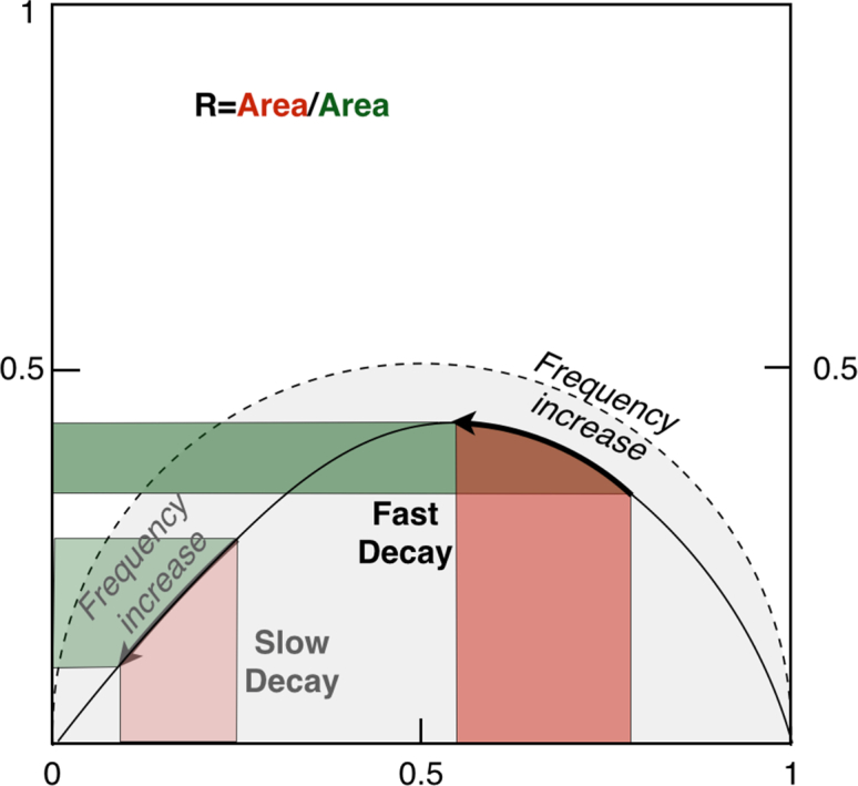
The phasor representation of multi-frequency lifetime measurement results from FmFLIM. The dashed half circle is the phasor trajectory of single exponential decay. All phasor trajectories, regradless decay models, should fall within the grey area surrounded by the dashed half circle. Red areas are imaginary projection areas of the trajectory over a given frequency sweeping span. Green areas are real projection areas.

To quantify the location and movement of the phasor during a frequency sweeping, we define a quantity R as the ratio between the imaginary projection area (red areas in Fig. 2) and the real projection area (green areas in Fig. 2)

$${\mathbf{R}}_{ij}=\frac{\Im {\int }_{{\omega }_{\mathit{max}}}^{{\omega }_{\mathit{min}}}{\tilde{I}}_{ij}^{\mathit{Cor}}({\omega }_i)d{\omega }_i}{\Re {\int }_{{\omega }_{\mathit{max}}}^{{\omega }_{\mathit{min}}}{\tilde{I}}_{ij}^{\mathit{Cor}}({\omega }_i)d{\omega }_i}$$ (5)

At the same modulation frequency, phasor of slow decays are located at the left side of the trajectory, and phasor of fast decays are located at the right side of the trajectory. Thus, slower decays have larger R-ratios and faster decays have smaller R-ratios. For example, when the decay of a fluorophore follows the single-exponential decay model, the complex phasor is given by

$$\tilde{I}(\omega )=\frac{\beta }{1+i\omega \tau }$$ (6)

where τ is the decay lifetime. Integrating Eq. (6) over a continuous frequency span yields

$$\begin{array}{lll}{\int }_{{\omega }_{\mathit{max}}}^{{\omega }_{\mathit{min}}}\tilde{I}(\omega )d\omega \hfill & =\hfill & \frac{\beta }{\tau }\left[{\text{tan}}^{-1}({\omega }_{\mathit{max}}\tau )-{\text{tan}}^{-1}({\omega }_{\mathit{min}}\tau )\right]\hfill \\ \hfill & \hfill & -\frac{i\beta }{2\tau }\left[\text{ln}\left({\omega }_{\mathit{max}}^2{\tau }^2+1\right)-\text{ln}\left({\omega }_{\mathit{min}}^2{\tau }^2+1\right)\right]\hfill \end{array}$$ (7)

The R-ratio is

$$\mathbf{R}(\tau )=\frac{\text{ln}\left({\omega }_{\mathit{max}}^2{\tau }^2+1\right)-\text{ln}\left({\omega }_{\mathit{min}}^2{\tau }^2+1\right)}{2\left[{\text{tan}}^{-1}\left({\omega }_{\mathit{max}}\tau \right)-{\text{tan}}^{-1}({\omega }_{\mathit{min}}\tau )\right]}$$ (8)

The function in Eq. (8) monotonically increases with the decay lifetime (Fig. 3(a)).

Fig. 3.

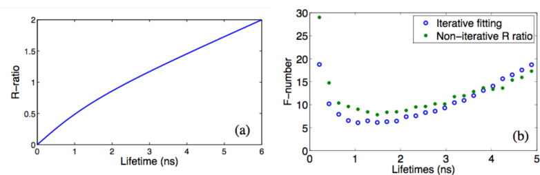
(a) Theoretical R-ratio of frequency-sweeping lifetime data, assuming single exponential decay. The curve is calculated with ω_min= 15 MHz and ω_max= 150 MHz. ω_min is limited by the low-pass band limit of RF electronics, and ω_max is limited by the maximal scan speed of the optical delay line as ${\omega }_{\mathit{max}}=\frac{2\pi {\lambda }_{\mathit{ex}}}{v_{\mathit{max}}}$ in FmFLIM [20].

(b) F-number of the iterative lifetime fitting method vs. the non-iterative R-method, calculated by Monte Carlo simulation [26, 27]. The F-number is defined as $\frac{\mathrm{\Delta }\tau }{\tau }\frac{N}{\mathrm{\Delta }N}$, where N is the detected photon number.

3.2. R-method: lifetime recovery from the R-ratio

Equation (8) and Fig. 3 define a look-up table between the experimentally measured R-ratio and a decay lifetime.The above lifetime recover method, named the R-method, requires minimal computation. In the case of single exponential decay, the average lifetime obtained through the R-method, should match the real decay constant. Its lifetime accuracy, quantified by the F-Number [26,27], is similar to that of iterative single-exponential decay fitting under identical fluorescent brightness (Fig. 3(b)).

In the case of multi-exponential decay, the lifetime obtained by the R-method represents an averaged lifetime of all components. We tested the R-method with simulated multi-exponential decay data. Figure 4 plots R-ratios of simulated FmFLIM data from mixtures of two lifetime components, and average lifetime results obtained by applying single-exponential fitting or the R-method on simulated data. Both methods can detect the increasing average lifetime when the fraction of long lifetime component increases. Differences in the average lifetime values between two methods are minimal. However, the R-method, been a non-iterative method, requires only simple arithmetic calculations, and can therefore be implemented in FPGA hardware for real-time determination of average fluorescence lifetimes at multiple Ex-Em spectral channels.

Fig. 4.

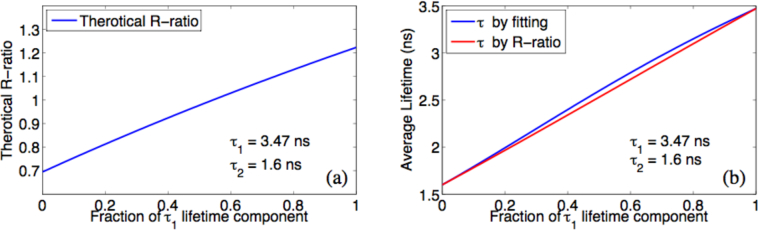
(a) R-ratio calculated from simulated data of a double-exponential decay sample, whose τ₁ = 3.47ns and τ₂ = 1.6ns.The fraction of τ₁ component increases from 0 to 100% (x-axis). (b) Average lifetimes obtained by single-exponential model fitting (blue) of simulated data or the R-method (red)

It worth noting that regardless of the decay model, the R-ratio always increases as the overall decay rate decreases. The ratio is the weighted average value of tan[ϕ(ω)] over a frequency span ω, using mcos[ϕ(ω)] as the weighting function. At any given modulation frequency, slower decays always have a larger phase lag ϕ than fast decays, thus the R-ratio will always increase when the decay constant increases in a single exponential decay, or the fraction of a long lifetime component increases in a multi-exponential decay. Practically, the R-ratio can be used as a quantitative indicator of the decay speed without assuming a particular decay model.

3.3. FPGA implementation of the R-method

The hardware implementation of the R-method is based on a LabView-programmable FPGA board (NI PXIe 7962, equipped with Xilinx Vertex-5 FPGA board). The available resources on the FPGA board are sufficient for parallel analysis of multiple Ex-Em channels. In the current implementation, approximately 70% of the FPGA’s logical resources are used to perform 8-channel real-time lifetime analysis with the R-method.

The FPGA process is divided into two main modules: data acquisition and data analysis, as sketched in Fig. 5 for a single Ex-Em channel. At each channel, the demodulated low frequency analog signal, which contains time-resolved fluorescence responses [13], is digitized at 50 MHz by a 16-bit multi-channel digitizer (NI 5752), and streamed into the acquisition module on the FPGA board, which is running at 50 MHz in sync with the digitizer. A trigger signal, which is synchronized with frequency sweeping and pixel scanning of the optical system, is also digitalized and sent to the acquisition module.

Fig. 5.

Diagram of FPGA-based lifetime image processing in the FmFLIM microscope. ADC: Analog-Digital Convertor. Clk: Clock. FIFO: First-in-first-ou buffer.

The FPGA acquisition module performs two functions: triggered acquisition and averaging down sample. For each pixel, the digitalized trigger signal is used to start 22-μs-long data acquisitions. The raw data stream is at 50 MHz per channel, set by the fixed sampling frequency of the digitizer. The 50-MHz sampling rate is unnecessarily high for detecting 200–250 kHz analog signals. Thus the raw data stream is down sampled to 2 MHz through averaging in the acquisition module. The final data stream consists of 44 frequency points per pixel per channel. The down-sampled data is streamed to the host computer and stored, so that iterative fitting could be performed offline if needed. In the meantime, the down-sampled data is also sent to the FPGA data analysis module through an internal FIFO for real-time lifetime imaging calculation.

The FPGA data analysis module is implemented in a parallel thread running at 40 MHz clock rate. The data analysis module performs two functions: calculating the signal intensity of the pixel, and calculating the R-ratio. The pixel intensity is calculated by summing the absolute value of the signal over all frequency points within the pixel. The R-ratio is calculated according to the procedure described in Section 3.1. For each spectral channel, the complex RF response of the channel is pre-calibrated with fluorescence lifetime standard solutions; the correction data are then pre-loaded into the FPGA block RAM from the host computer as an array during initialization. The real and imaginary parts of the correction data are stored as separate constant arrays. The 44-frequency-point data array within a pixel is divided by the corresponding real and imaginary part of the RF correction array. The real and imaginary multiplication results are then summed respectively to obtain the real and imaginary integrals in Eq. (5). At last, the imaginary integral is divided by the real integral to obtain the R-ratio.

Finally, the intensity and the R-ratio data are streamed to the host computer, where the fluorescence lifetime of the pixel is recovered from the R-ratio using the look-up table plotted in Fig. 3. Intensity and R-ratio images can be shown in real time on the FmFLIM confocal microscope’s imaging control program. The data acquisition and analysis for all 8 spectral channels run in parallel on the FPGA broad. Lifetime images of up to 8 Ex-Em channels can be displayed in real time.

4. Results: R-method vs. iterative fitting

4.1. Single exponential decay: GFP lifetimes in different refractive indices

The R-method was first tested on samples with single-exponential decay. GFP was dissolved in PBS that contains 0% to 80% glycerol, whose refractive indices changes from 1.33 to 1.44. Figure 6 plots lifetimes calculated by single-exponential fitting and by the R-method. Both results follows the τ⁻¹ ∝ n² rule [24] predicted by the Strickler-Berg formula [28]. Statistical lifetime errors between each 22-μs measurements are similar between two methods. Measurement errors, i.e., lifetime accuracies, of both methods are also similar, as the F-number analysis has predicted. The result proves that the R-method is equally effective as the iterative fitting method in quantifying the decay constant of single exponential decays.

Fig. 6.

GFP lifetime changes due to refractive index changes of media. Lifetimes are calculated by single-exponential fitting (blue) and the R-method (red). Error bars represent STDs of lifetimes from 40,000 repeating measurements, each acquired with a total acquisition time of 132 μs.

4.2. Multi-exponential decay lifetime standards

Practically, most FLIM samples contain multiple exponential decay components. Thus the R-method was then tested with standard samples of known multi-exponential decay constants [25]. These standards were double stranded DNA (dsDNA) oligonucleotides with single or double internal fluorescent labels. dsDNA were formed by hybridizing two single stranded DNA (ssDNA) oligonucleotides with complimentary sequences. When one of the ssDNA is labeled with fluorescein and the other is unlabeled, in the resulting dsDNA, the decay of fluorescein is a single exponential decay at τ = 3.47ns. When two ssDNA were internally labeled with either fluorescein or Cy3 respectively, in the resulting dsDNA, fluorescein and Cy3 are separated by 15 base pairs (sequences and labeling sites are shown in Fig. 7(a)). Because of the short distance between fluorescein and Cy3, strong FRET occurs and quenches the fluorescence lifetime of the donor (fluorescein) from 3.47 ns (in ssDNA) to 1.6 ns (in dsDNA) [29].

Fig. 7.

(a) The structure of dsDNA formed by complementary internally fluorescein-labeled 30-mer ssDNA and Cy3 labeled 66-mer ssDNA. The lifetime of fluorescein is 3.47 ns in ssDNA, and 1.60 ns in dsDNA due to FRET. (b) Average lifetimes obtained by iterative fitting (x-axis) vs. by the R-method (y-axis) from mixtures of ssDNA and dsDNA. The dashed diagonal line indicates that R-method results are identical to results of iterative fitting. Error bars represent STDs of lifetimes from 40,000 repeating measurements, each acquired with a total acquisition time of 132 μs.

Lifetime standards with multi-exponential decay were prepared by mixing fluorescein-Cy3-labeled and fluorescein-labeled dsDNA at various ratios. Average lifetimes of fluorescein in these mixtures, obtained by iterative fitting with the single-exponential decay model, vary from 1.60 ns to 3.47 ns.

Figure 7(b) compares average fluorescein lifetimes of standards obtained by the R-method with those obtained by single-exponential iterative fitting. When the fluorescein emission is purely from fluorescein-Cy3-labeled dsDNA and the decay is single exponential, both the R-method and the iterative fitting method yield a lifetime of 1.6 ns. When the fluorescein emission is from a mixture of fluorescein-Cy3-labeled and fluorescein-labeled dsDNA, the decay is double exponential, and results from both methods are still close within measurement errors.

4.3. Timelapse imaging of cAMP FRET sensor

To demonstrate that the R-method has sufficient sensitivity for monitoring lifetime changes in live cells, we performed time-lapse cAMP imaging in HeLa cells expressing GFP-Epac-mCherry FRET sensor [25]. The FRET efficiency of the sensor is expected to decrease upon binding with cAMP. A drug treatment that increases cAMP (100 μM IBMX and 25 μM forskolin [25, 30]) was applied to cells during imaging.

Figure 8 plots the average lifetime timelapse traces of HeLa cells (N=4) expressing the cAMP sensor, in comparison to control HeLa cells (N=4) expressing free GFP. Average lifetimes obtained by single-exponential fitting and by the R-method match well. Both methods detected the GFP lifetime increase in the cAMP cells after treatment, whereas GFP lifetimes in the control cells remained constant. The result shows clearly the R-method is a reliable way to detect lifetime changes due to FRET in live cells.

Fig. 8.

Average GFP lifetime traces of HeLa cells (N=4) expressing the GFP-Epac-mCherry cAMP sensor, in comparison to HeLa cells (N=4) expressing free GFP. The treatment was applied at 5 minutes after imaging started. The cAMP level increased after the treatment, and GFP lifetimes of GFP-Epac-mCherry sensors increased accordingly. The lifetime of control cells expressing free GFP remained the same. Left y-axis: Average lifetimes. Right y-axis: Experimental R-ratio. Average lifetimes obtained by single-exponential fitting (blue) and by the R-method (red) match well.

The FmFLIM system is capable of performing lifetime imaging on multiple Ex-Em channels in a truly parallel fashion. With the R-method, multi-channel lifetime images can be calculated in real time. Figure 9 shows two-channel lifetime images of HeLa cells expressing the cAMP sensor, which were acquired with two CW lasers (488 nm and 561 nm) at the same time. One channel (Ex: 488 nm, Em: 525±20 nm) measured the lifetime of GFP, which was expected to increase when cAMP level increases, and the acceptor channel (Ex: 561, Em: 593±20nm), which detected the self-excitation-emission of mCherry and was not expected to change because fluorescent signals in this channel are unrelated to the FRET process. Experimental results calculated by the R-method matched expectations. Lifetime images clearly demonstrated that the donor lifetime increased due to the treatment. In the meantime, the acceptor lifetime was undisturbed because the acceptor self excitaiton-emission is independent of the FRET process. These results verified that lifetime calculated by the R-method is highly reliable and sensitive, and the R-method is capable of capturing dynamic lifetime changes in live cells.

Fig. 9.

Time-lapse cAMP level imaging of HeLa cells expressing GFP-Epac-mCherry sensor. FLIM confocal images were taken at the donor (GFP) channel (Ex: 488 nm, Em: 525±20 nm) and the acceptor (mCherry) channel (Ex: 561, Em: 593±20nm) simultaneously. Lifetime images were calculated with the R-method.

(a) Multi-channel FLIM images before treatment. a1: false color image of donor (GFP, green) and acceptor (mCherry, red) brightness. a2: Lifetime image of the donor channel. a3: Lifetime image of the acceptor channel.

(b) Multi-channel FLIM images after treating with IBMX and forsklin, which increased cellular cAMP level. b1: false color image of donor (GFP, green) and acceptor (mCherry, red) brightness. b2: Lifetime image of the donor channel, showing the donor lifetime increased. b3: Lifetime image of the acceptor channel, showing unchanged acceptor channel lifetime. The acceptor channel is unrelated to the FRET process, and lifetimes in this channel is unaffected by the treatment.

(c) Pixel histogram of the donor before and after the treatment. Increased donor lifetime indicates a higher cAMP level after the treatment.

(b) Pixel histogram of the acceptor channel before and after the treatment. The acceptor channel lifetime is undisturbed as expected.

5. Summary

The purpose of developing a non-iterative lifetime analysis methods is to speed up lifetime computing of FLIM data, and to enable hardware-based lifetime image analysis. The latter is extremely important for the Fourier multiplexed FLIM (FmFLIM) technique, which is capable of acquiring fast time lapse FLIM image on multiple channels. In the past, applications of this novel parallel multiplexed FLIM technique was hampered by the large computation load coming from iterative fitting of multi-channel lifetime images. This paper establishes the R-method for frequency-sweeping FmFLIM. Experimental tests proved that the performance of the R-method is equivalent to that of single-exponential iterative fitting, and the sensitivity and reliability of the R-method are well suited for time-lapse FLIM-FRET imaging of live cells. With the R-method and its FPGA implementation, multi-channel lifetime images can now be generated in real time on the frequency-sweeping FmFLIM system. The advance will greatly facilitate the application of FmFLIM in biomedical research.