The utility of Bayesian predictive probabilities for interim monitoring of clinical trials

Abstract

Background

Bayesian predictive probabilities can be used for interim monitoring of clinical trials to estimate the probability of observing a statistically significant treatment effect if the trial were to continue to its predefined maximum sample size.

Purpose

We explore settings in which Bayesian predictive probabilities are advantageous for interim monitoring compared to Bayesian posterior probabilities, p-values, conditional power, or group sequential methods.

Results

For interim analyses that address prediction hypotheses, such as futility monitoring and efficacy monitoring with lagged outcomes, only predictive probabilities properly account for the amount of data remaining to be observed in a clinical trial and have the flexibility to incorporate additional information via auxiliary variables.

Limitations

Computational burdens limit the feasibility of predictive probabilities in many clinical trial settings. The specification of prior distributions brings additional challenges for regulatory approval.

Conclusions

The use of Bayesian predictive probabilities enables the choice of logical interim stopping rules that closely align with the clinical decision making process.

1 Introduction

Interim monitoring is an important component of most randomized clinical trials. Phase II clinical trials often use multi-stage designs such as Simon’s two-stage design [1, 2]. Phase III designs typically use group sequential designs with alpha and beta-spending functions, such as O’Brien and Fleming [3] and Pocock [4]; see DeMets [5], and Thall and Simon [6] for more comprehensive reviews. Bayesian methods can also be useful for interim monitoring, often basing decisions of stopping on whether the posterior probability of a parameter exceeds a pre-specified threshold. Examples include Thall and Simon [7, 8], Sylvester [9], Heitjan [10], and Tan and Machin [11]. For discussions comparing Bayesian to frequentist designs in the context of clinical trials, see Spiegelhalter et al. [12], Berry [13-16], Stangl and Berry [17], and Lee and Chu [18].

These methods employ various metrics for assessing evidence at an interim analysis. Such metrics include (but are not limited to) the p-value, the probability of observing a result as extreme or more extreme than the observed result under the null hypothesis; a Bayesian posterior probability, typically expressed as the probability the parameter is contained within a meaningful region; conditional power, the frequentist probability of obtaining statistical significance at some future sample size given the current data and assumed parameter value(s); and Bayesian predictive probability, the probability of obtaining statistical significance at some future sample size given the current data and assumed prior distribution(s). The choice of metric is ideally a function of the purpose of the interim analysis.

Two common types of questions addressed by interim analyses include 1) Is there convincing evidence in favor of the null or alternative hypotheses? and 2) Is the trial likely to show convincing evidence in favor of the alternative hypothesis if additional data are collected? The first question pertains to the evidence presently shown by the data, and is best addressed using estimation, p-values, or Bayesian posterior probabilities. The second deals with prediction of what evidence will be available at later stages in the study, and is best addressed using stochastic curtailment methods such as conditional power or predictive probability.

Conditional power [19, 20] is often criticized for assuming the unknown parameters are fixed at specific values [21, 18, 22]. In contrast, Bayesian predictive probabilities average the probability of trial success over the variability in the parameter estimates, and can be used whether the trial’s primary analysis is frequentist [23-26] or Bayesian [27-32]. They are most often used to predict trial success at a final pre-determined sample size, but can also be used to predict trial success based on an interim sample size with extended follow-up [33-35]. Predictive probabilities have been widely discussed in the literature [21]. However, the literature lacks a general discussion of the advantages of predictive probabilities for interim monitoring. This article contrasts predictive probabilities versus traditional methods for interim monitoring of clinical trials. We illustrate settings in which predictive probabilities have advantages over more traditional methods of interim monitoring, particularly in the context of futility monitoring and efficacy monitoring with lagged outcomes (Sections 2-4). We also explore the relationship between the predictive probability and posterior probability (Section 5) and conclude with a discussion.

2 Monitoring for futility

There are many reasons for interim monitoring of clinical trials. Perhaps the greatest reason is the ethical imperative to avoid treating patients with ineffective or inferior therapies. However, oftentimes there are not sufficient data at an interim analysis to make a definitive conclusion about treatment benefit. In such cases, a more relevant question may be whether a trial is likely to reach a definitive conclusion by the end of the study. If not, many would argue that it is unethical to continue enrolling patients and that accrual should be stopped due to trial futility so that resources (monetary, personnel and available trial patients) can be allocated to other investigational therapies. If futility is defined as a trial being unlikely to achieve its objective [36], then futility is inherently a prediction problem, and is best addressed using predictive probabilities and not posterior probabilities or p-values. The main reason is that the amount of time and statistical information remaining to be collected are key determinants in the probability of obtaining a statistically significant result (i.e. trial success).

For example, consider a single-arm study with a maximum of 100 patients measuring a binary outcome response, in which the proportion of successes is compared to a gold standard with a 50% response. The outcome observed is the number of responses x, which is assumed to follow a binomial distribution with probability of response p and total number of patients N = 100. The trial will be considered a success if the Bayesian posterior probability that the proportion exceeds the gold standard (p₀ = 0.5) is greater than η = 0.95 as given by (1).

$$\mathrm{Pr}(p>p_0\mid x)>\eta$$ (1)

If a uniform prior p ~ Beta(α₀ = 1, β₀ = 1) is specified, the trial will be considered a success if 59 or more of 100 patients observe a response, where Pr(p > 0.50∣x = 59, n = 100) = 0.963. Furthermore, this non-informative prior and cut-off conserves Type I error: the probability of erroneously rejecting the null hypothesis if p = 0.5 is 0.044. A frequentist exact binomial test also requires 59 or more successes to achieve statistical significance at the one-sided 0.05 level.

2.1 Predictive probabilities compared to p-values and posterior probabilities

Suppose the trial is designed with four planned interim analyses for futility which are conducted when data are available for 20, 50, 75, and 90 patients, respectively. Suppose at the first interim analysis 12 responses out of 20 patients (60%) are observed (exact one-sided p-value = 0.25), such that 47 or more responses are needed in the remaining 80 patients in order for the trial to be a success. Under a uniform prior, the Bayesian posterior probability of interest is Pr(p > 0.50∣x₁ = 12, n₁ = 20) = 0.81. The Bayesian posterior predictive distribution of future observations y₁ follows a beta-binomial distribution, i.e. y₁ ~Beta-binomial(50, α = α₀+12, β = β₀+8), and the predictive probability of success equals 0.54, which is the probability of observing 47 or more responses in the remaining 80 patients given the observed data.

Suppose the second, third, and fourth interim analyses yield 28 successes/50 (56%), 41/75 (55%), and 49/90 (54%), with posterior probabilities of 0.81, 0.79, 0.80 and p-values of 0.24, 0.24, and 0.23, respectively. Given these nearly identical summaries of evidence for treatment benefit, it is not obvious whether the trial should be stopped or continued at each of the interim analyses. Note the posterior distribution at n = 20 observations has a much larger variance than the posterior distribution at n = 75 (Figure 1), but one cannot easily distinguish between the different probabilities of trial success by examining the posterior distributions or posterior probabilities alone.

Figure 1.

Bayesian posterior distributions for 4 interim analyses with x responses of n observations and maximum sample size N= 100; comparing predictive probability of success, posterior probability Pr(p > 0.50∣x, n), and one sided p-value for H₀ : p = 0.5

In contrast, the predictive probabilities vary dramatically across the interim looks, with values of 0.54, 0.30, 0.086, and 0.003 at 25, 50, 75, and 90 patients, respectively (Table 1). Many would agree that this trial should be stopped at 75 patients due to a 0.086 probability of trial success. The specific stopping criteria are typically unique to each trial, and include ethical and business considerations, such as risk/benefit considerations of patients, available resources, opportunity cost, and overall statistical power. For clarity, Table (2) gives explicit definitions of predictive probability and other measures being discussed within this illustrative example. In the context of interim monitoring for futility, predictive probabilities are naturally appealing because they directly address the relevant question, that is, whether a trial is likely to reach its objective if continued to the planned maximum sample size. Because of their natural interpretation, predictive probabilities have been used frequently for futility analyses in Bayesian adaptive trials. Examples include a three-arm Bayesian adaptive comparative effectiveness trial in refractory status epilepticus [37], a trial evaluating a rapid molecular test of early-stage breast cancer [38], and a cardiovascular safety study of a testosterone gel in postmenopausal women with hypoactive sexual desire disorder [34].

Table 1.

Illustrative example

nj	xj	mj	$y_j^{\ast }$	p-value	Pr(p > 0.5)	CPHa	CPMLE	PP
20	12	80	47	0.25	0.81	0.90	0.64	0.54
50	28	50	31	0.24	0.80	0.73	0.24	0.30
75	41	25	18	0.24	0.79	0.31	0.060	0.086
90	49	10	10	0.23	0.80	0.013	0.002	0.003

n_j and x_j are the number of patients and successes at interim analysis j

m_j = number of remaining patients at interim analysis j

$y_j^{\ast }$ = minimum number of successes required to achieve success

CP_Ha and CP_MLE: Conditional power based on original H_a or MLE

PP= Bayesian predictive probability of success

Table 2.

Definitions of key measures & methods for illustrative example

Measure/Method	Description	Formula
P-value	Probability of observing a proportion equal to or greater than x/n given H0 : p = p0	${\sum }_{i=x}^n\left(\begin{array}{l}n\\ i\end{array}\right)p_0^i{(1-p_0)}^{n-i}$
Posterior probability	Bayesian posterior probability that proportion exceeds the null value p0	$\mathrm{Pr}(p>p_0\mid x)={\mathit{\int }}_{p_0}^{1}f(x\mid p)\pi (p)/f(x)\mathit{dp}$
Predictive probability	Bayesian predictive probability of statistical significance at N given x/n and π(p)	${\sum }_{y=0}^m[I\{\mathrm{Pr}(p>p_0\mid x,y,N)>\eta \}f(y\mid x)]$
Conditional power	Frequentist probability of statistical significance at N given x/n and assumed $p_0^{\ast }$	${\sum }_{y=0}^m\left[I\left\{{\sum }_{i=x+y}^N\left(\begin{array}{c}N\\ i\end{array}\right)p_0^i{(1-p_0)}^{N-i}<\alpha \right\}f(y\mid p^{\ast })\right]$
Repeated testing of H1	Method of monitoring for futility based on p-value for test of alternative hypothesis	$\mathit{P}­\mathrm{value}={\sum }_{i=0}^x\left(\begin{array}{c}n\\ i\end{array}\right)p_1^i{(1-p_1)}^{n-i}$
Group sequential	Frequentist design for interim monitoring that allocates Type I/II errors across interim analyses	Varies by method
Stochastic curtailment	Method that estimates the probability of statistical significance at some future sample size	Varies by method

n and N are the number of patients at interim and final sample sizes, respectively

m = N − n: number of remaining patients yet to be observed in the study

x: number of successes observed at the interim analysis

y: number of successes yet to be observed in the remaining m patients

p₀ and p₁: proportion of successes under the null hypothesis and alternative hypotheses

p*: estimated or assumed value of p required for conditional power computation

α and η: criteria required to demonstrate “statistical significance” for p-value or posterior probability, respectively

I(): indicator function taking the value 1 if expression is true and 0 if otherwise

π(p) = Beta(1, 1) = 1: Prior distribution of p, uniform over (0,1)

$f(x)={\mathit{\int }}_0^{1}f(x\mid p)\pi (p)\mathit{dp}$: Marginal likelihood or normalizing constant

$f(y\mid x)={\mathit{\int }}_0^{1}f(y\mid p)f(p\mid x)\mathit{dp}={\mathit{\int }}_0^{1}f(y\mid p)f(x\mid p)\pi (p)/f(x)\mathit{dp}=\mathrm{Beta}­\mathrm{binomial}(m,1+x,1+n-x)$: Bayesian posterior predictive distribution of y given x

$f(x\mid p)=\left(\begin{array}{l}n\\ x\end{array}\right)p^x{(1-p)}^{n-x}$: Data likelihood of x given p for n patients observed by interim

$f(y\mid p)=\left(\begin{array}{l}m\\ y\end{array}\right)p^y{(1-p)}^{m-y}$: Data likelihood of y given p for remaining m patients

2.2 Frequentist strategies of monitoring futility

Group sequential trials and their funnel shaped boundaries acknowledge the reality that decisions based on interim p-values depend on the amount of information yet to be observed. This implies that p-values (and posteriors) require additional information for decision making regarding futility, and thus their boundaries necessarily change at each interim analysis. DeMets [39] provides a brief summary of different types of methods available for monitoring trials for futility. Group sequential methods are designed with the goal of optimizing allocation of Type I or Type II error, and are not designed to monitor the probability of trial success. Despite this fact, they are often used for monitoring futility, even when futility is defined as a trial being unlikely to achieve its objective. One such example is the Emerson & Fleming symmetric boundary [40], which is a special case of the more general Unifying Family proposed by Kittelson and Emerson [41]. Consider the use of the Emerson & Fleming lower boundary in the above example, in which the trial is monitored for futility at 20, 50, and 75 patients, with a final analysis for efficacy at 100 patients. The test of interest is a one-sided test of H₀ : p ≤ 0.5 vs. H₁ : p > 0.5, with a Type I error of 0.05. The trial will stop for futility if less than 5 successes/20 (25%), 25/50 (50%), 42/75 (56%), or 59/100 (59%) are observed. The power of the above design for an alternative of p₁ = 0.65 is 0.93. Using our Bayesian model with uniform priors, the predictive probabilities of success at 5, 25, and 42 successes at the first three interim looks (which would not meet the above stopping rules) are 0.0004, 0.041, and 0.188. In the context of monitoring futility as defined above, the decision rules for futility produced by the Emerson and Fleming boundaries are suspect, as trials with very low probabilities of success would be allowed to continue.

A related but distinct strategy is given by Fleming et al. [42] and Anderson and High [43], where one repeatedly tests the alternative hypothesis at some significance level (typically 0.005), and rejects the alternative hypothesis if the data are inconsistent with the assumed alternative. Because such methods are appropriately using estimation methods to evaluate evidence against a specific hypothesis, they may have more intuitive appeal than the beta-spending group sequential methods. However, assessing evidence against the alternative hypothesis does not directly assess whether the trial will meet its objective. If we apply this approach to our illustrative example using the 0.005 significance level and include the extra look at 90 patients, we will stop for futility if less than 8 responses/20 (40%), 24/50 (48%), 38/75 (51%), or 47/90 (52%) are observed. The corresponding predictive probabilities of success at 8, 24, 38, and 47 responses (which would allow the trial to continue) are 0.031, 0.016, 0.002, and 0.0, respectively. The above rules will allow trials to continue even despite having very small (or even zero) probabilities of success. Such futility designs can be made more aggressive or conservative by varying the significance levels or Type II error probabilities (e.g. using 0.02 instead of 0.005 [44]), but it’s not obvious whether such rules reflect good judgment from a futility decision-rule standpoint. Such methods do have some appeal if futility is defined as a trial being unlikely to observe the effect it was designed to detect, but such a definition requires the specification of a subjective alternative hypothesis (e.g. p₁ = 0.65) which raises numerous issues [36].

Additionally, frequentist approaches such as Simon’s two-stage design [1, 2], that minimize expected sample size for single-arm studies with a single interim analysis, are difficult to use when the number of patients accrued is not fixed [44]. Strategies halting accrual if a positive effect is not observed at 50% information [45, 46] do not accommodate multiple interim analyses.

2.3 Conditional Power

In contrast to the above frequentist strategies, interim analyses for futility based on conditional power attempt to account for how many data remain to be observed via stochastic curtailment. In order to calculate conditional power, one must assume that some value of a parameter is the truth, which of course is unknown in a real trial. Consider the working example. Under an initial assumption of a 65% response rate, 100 patients provide about 90% power for a one-sided exact binomial test, with a type I error rate of 0.05. Table 1 shows the conditional power based upon the initial effect size estimate CP_Ha and upon the observed interim maximum likelihood estimate CP_MLE. During the course of the above trial, the probability that 65% is the true success rate continually decreases, but CP_Ha continues to use the hypothesized rate of 0.65 despite this shrinking reality. CP_MLE uses the maximum likelihood estimate at each analysis but fails to incorporate the variability of that estimate.

The variability is particularly important because the relationship between power and effect size is concave down for higher powers, concave up for lower powers, and is not symmetric about the MLE. This is evident in Figure 2, which shows the conditional probability of achieving 59 or more successes at N = 100 given 12 success in 20 subjects (solid line) as a function of the true (but unknown) success rate. For example, assuming p = 0.65 (the original design assumption) or 0.60 (current MLE), the graph shows a 0.90 or 0.64 probability of a successful trial, respectively. The use of the MLE (0.60) or original assumption of 0.65 can be misleading because the power curve flattens out more quickly to the right of those values than it does to the left.

Figure 2.

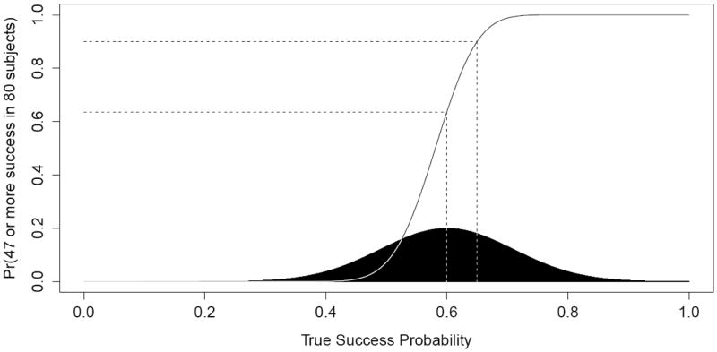
Conditional power of successful trial at N = 100 (solid line) by (assumed) true success probability compared to interim posterior distribution of response probability p (shaded region), given x₁ = 12 successes in n₁ = 20 subjects

A typical strategy for trials that incorporate conditional power is to provide estimates under various alternatives, e.g. under the null hypothesis, the original H_a, and the interim MLE. This is essentially an informal attempt to average the conditional power over various alternatives, reffecting the uncertainty in the choice of the true alternative. In contrast, predictive probabilities explicitly integrate the conditional power over the current posterior, shown in black at the bottom of Figure 2. Of course the predictive probability is dependent on the chosen prior, which may have a large influence for small sample sizes such as 20 enrolled patients (see Discussion for further discussion of priors).

3 Monitoring for efficacy

A decision of stopping early for efficacy is typically based on whether there is convincing evidence at an interim analysis in favor of the alternative hypothesis, which is best addressed using estimation, p-values, or posterior probabilities. However, prediction methods can be advantageous for monitoring efficacy and stopping accrual when there is a time lag between enrollment and the observed outcomes (e.g. see [33, 34, 35]). This time lag is present in nearly all clinical trials. For example, suppose the outcome is response to treatment in the first 90 days. Rather than base efficacy decisions on the interim posterior probability with incomplete data for enrolled patients, one can estimate the predictive probability of success if all enrolled patients with unobserved outcomes were followed the full 90 days. If this probability is sufficiently large, one can stop enrollment (permanently) and wait 90 days before conducting a superiority analysis. Numerous Bayesian adaptive trials with lagged primary outcomes use this methodology, e.g. trials described in Skrivanek et al. [47] and White et al. [34] both stopped accrual early for predicted success.

In frequentist settings, it is common practice to use group sequential methods at an interim analysis using only patients with complete data. If the trial is stopped due to a stopping boundary being met, sometimes a final analysis is done after all lagged outcomes are collected on the current set of patients. In such settings, trial success is determined by the interim analysis and not the subsequent final analysis, although the data monitoring committee (DMC) may have reservations for stopping a trial early if a few lagged outcomes can affect the p-value such that it no longer meets the group sequential boundary. Bayesian predictive probabilities formalize the decision to stop accrual in a manner consistent with the decision process of the DMC, i.e. only stopping trials for efficacy if they currently show superiority and will likely maintain superiority after the remaining data are collected.

4 Prediction via auxiliary variables

Another advantage of using predictive probabilities for monitoring efficacy is the ability to model a final primary outcome using earlier information that is informative about the final outcome [48]. For example, if the primary outcome is success at 24 months, many of the accrued patients at a given interim analysis will not have 24 months of observation. However, one may have access to a measure of success at 3, 6, or 12 months that correlates with the outcome at 24 months. Such auxiliary variables [48] may not be valid endpoints from a regulatory perspective, but the correlation between the auxiliary variables and the final outcome can be incorporated into the predictive distribution of the final outcome to provide a more informative predictive probability of trial success.

If the predictive probability of success at the maximum sample size is sufficiently small, the trial can be stopped for futility immediately. If the predictive probability of success at complete information for currently accrued patients is sufficiently large, one can stop accrual and wait until the primary outcome is observed for all currently enrolled patients (or wait a specified time for time-to-event outcomes), at which point trial success is evaluated. In this setting, the auxiliary variables do not contribute to the final analysis; rather they are used to inform the predictive probability that would either stop the trial for futility or stop trial accrual in anticipation of success. This is a great advantage of predictive probabilities over competing methods for interim monitoring (group sequential, conditional power, p-values, posterior probabilities, etc.), where properly accounting for auxiliary variables or time lags between enrollment and observed outcomes is much more difficult.

5 Relationship between predictive probability of success and posterior probability of efficacy

When an infinite amount of data remain to be collected at an interim analysis, the predictive probability of success of the trial equals the current posterior estimate of efficacy, Pr(p > p₀∣x, n), regardless of the posterior cutoff η (equation 1) required for a trial to be a success. In our illustrative example, the rate of convergence is a function of the number of responses observed, the null value p₀, and the posterior cutoff η. Larger values of η, e.g. 0.90, have a slower rate of convergence to the posterior estimate than smaller values, e.g. 0.70 (see Figure 3). However, for a trial with a fixed sample size N, the estimated predictive probabilities will typically be closer to the posterior estimates at the beginning of a trial, and move toward either 0 or 1 as the trial nears completion (see Figure 4).

Figure 3.

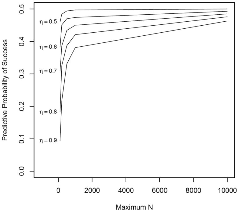
Predictive probability of success vs. maximum sample size N by posterior threshold η, with interim n = 50 and observed x = 25

Figure 4.

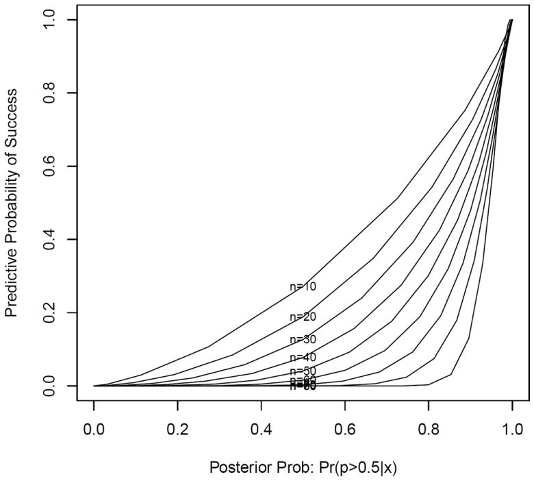
Predictive probability of success vs. posterior estimate Pr(p > 0.50∣x) by interim sample size n, with maximum sample size N = 100 and posterior threshold η = 0.95

As noted by Emerson et al. [22], there is a 1:1 correspondence between various boundary stopping scales. For example, consider a trial with three interim analyses at 10, 50, and 75 patients, in which the maximum N = 100 and posterior cutoff η = 0.95, and the trial is stopped early if the predictive probability of success is less than 0.20 at any of the interim analyses. An identical design based on posterior probabilities will stop the trial if the posterior estimate of efficacy is less than 0.577 (12/20 or less), 0.799 (28/50 or less), or 0.897 (42/75 or less) for the three interim looks, respectively. Hence, the posterior rule must vary across the interim analyses to produce identical decisions as the predictive probability approach with a fixed cut-off. Although such a 1:1 correspondence was evident in this example, it is often difficult to align the posterior and predictive probability rules. Note it would also be straightforward to define meaningful efficacy and futility bounds with varying predictive probability boundaries (with ethical or efficiency based justifications).

6 Discussion

As discussed by Berry [16], one can design a Bayesian approach that delivers pre-determined frequentist operating characteristics, such as 90% power with a false positive rate of 5%, to comply with regulatory agencies such as the FDA. Such Bayesian strategies for building frequentist designs can still deliver benefits compared to traditional frequentist methods, especially through the use of predictive probabilities. For example, a DMC could use a predictive probability of success to help inform decisions for a frequentist trial with no planned interim monitoring [16]. In addition, Bayesian predictive probabilities can be used for monitoring purely frequentist trials, and for conducting seamless phase II/III studies in which the predictive probability of phase III efficacy is calculated within the phase II study before transitioning to the phase III [47]. Berry [15] states that the concept of “predictive probability is an enormously important contribution of the Bayesian approach. Without it, the Bayesian approach would be much less compelling.”

The design of trials with interim monitoring via Bayesian predictive probabilities often requires intensive computer simulations [49], which involves repeated sampling of future observations from the posterior predictive distribution. The computational burden is magnified when assessing operating characteristics in the design stage, because the predictive probability calculation may be needed for each interim analysis within every simulated trial for each set of parameter settings. As high performance computers continue to improve in efficiency and Bayesian software becomes more available, we anticipate this issue will gradually lessen over time.

Emerson et al. [22] argue that the choice of scale for the stopping rule is immaterial so long as the operating characteristics of the stopping rule are adequately addressed, but that predictive probability or stochastic curtailment cannot accurately predict the impact of a stopping rule on statistical power or efficiency. While we agree that power and efficiency are important factors, trials must also reflect good judgment. Continuing a trial that has a very small probability of success may not be considered an ethically sound decision, even with optimized frequentist operating characteristics. Friedlin and Korn [36] also discuss instances in which group sequential boundaries would stop a trial early, even though the predictive probability of success is reasonably high.

Emerson et al. [22] also criticize the use of predictive probabilities for interim monitoring due to the uncertainty in the specification of the prior distribution. This is not a criticism specific to predictive probabilities, but of Bayesian methods in general. Clinical trial designs using predictive probabilities for interim monitoring do not claim efficacy using predictive probabilities. Rather, the claim of treatment benefit is based on either Bayesian posterior probabilities or frequentist criteria such as p-values. Hence, the same discussions of prior distributions in the literature [17, 48, 50, 51] are applicable to Bayesian designs with interim monitoring via predictive probabilities.

Dmitrienko and Wang [21] discuss the choice of prior distributions specifically in the context of interim monitoring via predictive probabilities. They show that flat (or weak) priors can result in high early termination rates that may not be acceptable for many applications, and argue for stronger aggressive priors for futility monitoring when early stopping is undesirable, and that flat priors be used primarily for efficacy monitoring. The prior used for the predictive probability calculation need not match the prior used for the final analysis [48]. For example, a predictive probability of trial success at an interim analysis may use historical prior information while the final analysis uses a flat or skeptical prior. Such a strategy attempts to use all available information to more accurately predict whether the trial will be a success, but maintains objectivity or skepticism for determining efficacy.

Finally, all trial designers are informal Bayesians when calculating sample size, needing to use historical data and expert opinion to estimate effect size and its variability. It is inconsistent to criticize Bayesian predictive probabilities for depending on a well-constructed prior (while also incorporating current within-trial data), yet suggest that a better approach is to rely on initial, precise guesses of effect size and population variability in the face of accumulating contrary evidence within the trial.

In summary, we have illustrated settings in which Bayesian predictive probabilities have advantages for interim monitoring of clinical trials, specifically in the context of futility monitoring and efficacy monitoring with lagged outcomes. We advocate that more trials use predictive probabilities for interim monitoring for addressing hypotheses related to prediction, which if implemented correctly will lead to better designs and decisions in the practice of clinical trials.

References

- 1.Simon R. Optimal two-stage designs for phase II clinical trials. Controlled Clinical Trials. 1989;10:1–10. doi: 10.1016/0197-2456(89)90015-9. [DOI] [PubMed] [Google Scholar]
- 2.Lee JJ, Feng L. Randomized phase II designs in cancer clinical trials: current status and future directions. Journal of Clinical Oncology. 2005;23:4450–4457. doi: 10.1200/JCO.2005.03.197. [DOI] [PubMed] [Google Scholar]
- 3.O’Brien PC, Fleming TR. A multiple testing procedure for clinical trials. Biometrics. 1979;35:549–556. [PubMed] [Google Scholar]
- 4.Pocock SJ. Group sequential methods in the design and analysis of clinical trials. Biometrika. 1977;64:191–199. [Google Scholar]
- 5.DeMets DL. Interim Analysis: The alpha spending function approach. Statistics in Medicine. 1994;13:1341–1352. doi: 10.1002/sim.4780131308. [DOI] [PubMed] [Google Scholar]
- 6.Thall PF, Simon R. Recent developments in the design of phase II clinical trials. Cancer Treatment and Research. 1995;75:49–71. doi: 10.1007/978-1-4615-2009-2_3. [DOI] [PubMed] [Google Scholar]
- 7.Thall PF, Simon R. A Bayesian approach to establishing sample size and monitoring criteria for phase II clinical trials. Controlled Clinical Trials. 1994;15:463–481. doi: 10.1016/0197-2456(94)90004-3. [DOI] [PubMed] [Google Scholar]
- 8.Thall PF, Simon R. Practical Bayesian guidelines for phase IIB clinical trials. Biometrics. 1994;50:337–349. [PubMed] [Google Scholar]
- 9.Sylvester RJ. A Bayesian approach to the design of phase II clinical trials. Biometrics. 1998;44:823–836. [PubMed] [Google Scholar]
- 10.Heitjan DF. Bayesian interim analysis of phase II cancer clinical trials. Statistics in Medicine. 1997;16:1791–1802. doi: 10.1002/(sici)1097-0258(19970830)16:16<1791::aid-sim609>3.0.co;2-e. [DOI] [PubMed] [Google Scholar]
- 11.Tan SB, Machin D. Bayesian two-stage designs for phase II clinical trials. Statistics in Medicine. 2002;21:1991–2012. doi: 10.1002/sim.1176. [DOI] [PubMed] [Google Scholar]
- 12.Spiegelhalter DJ, Freedman LS, Parmar MK. Bayesian approaches to randomized trials. Journal of the Royal Statistical Society, Series A. 1994;157:357–416. [Google Scholar]
- 13.Berry DA. Interim Analyses in Clinical trials: Classical vs. Bayesian Approaches. Statistics in Medicine. 1985;4:521–526. doi: 10.1002/sim.4780040412. [DOI] [PubMed] [Google Scholar]
- 14.Berry DA. A case for Bayesianism in clinical trials. Statistics in Medicine. 1993;12:1377–1393. doi: 10.1002/sim.4780121504. [DOI] [PubMed] [Google Scholar]
- 15.Berry DA. Bayesian Statistics and the Efficiency and Ethics of Clinical Trials. Statistical Science. 2004;19:175–187. [Google Scholar]
- 16.Berry DA. Bayesian clinical trials. Nature Reviews Drug Discovery. 2006;5:27–36. doi: 10.1038/nrd1927. [DOI] [PubMed] [Google Scholar]
- 17.Stangl DK, Berry DA. Bayesian statistics in medicine: Where are we and where should we be going? The Indian Journal of Statistics. 1998;60:176–195. [Google Scholar]
- 18.Lee JJ, Chu CT. Bayesian clinical trials in action. Statistics in Medicine. 2012;31:2955–2972. doi: 10.1002/sim.5404. [DOI] [PMC free article] [PubMed] [Google Scholar]
- 19.Lan KKG, Simon R, Halperin M. Stochastically curtailed tests in long-term clinical terms. Communications in Statistics. 1982;1:207–219. [Google Scholar]
- 20.Betensky RA. Early stopping to accept H0 based on conditional power: approximations and comparisons. Biometrics. 1997;53:794–806. [PubMed] [Google Scholar]
- 21.Dmitrienko A, Wang MD. Bayesian predictive approach to interim monitoring in clinical trials. Statistics in Medicine. 2006;25:2178–2195. doi: 10.1002/sim.2204. [DOI] [PubMed] [Google Scholar]
- 22.Emerson SS, Kittelson JM, Gillen DL. On the Use of Stochastic Curtailment in Group Sequential Clinical Trials. University of Washington; 2005. [Google Scholar]
- 23.Choi SC, Smith PJ, Becker DP. Early decision in clinical trials when the treatment differences are small. Experience of a controlled trial in head trauma. Controlled Clinical Trials. 1985;6:280–288. doi: 10.1016/0197-2456(85)90104-7. [DOI] [PubMed] [Google Scholar]
- 24.Spiegelhalter DJ, Freedman LS, Blackburn PR. Monitoring clinical trials: conditional or predictive power? Controlled Clinical Trials. 1986;7:8–17. doi: 10.1016/0197-2456(86)90003-6. [DOI] [PubMed] [Google Scholar]
- 25.Choi SC, Pepple PA. Monitoring clinical trials based on predictive probability of significance. Controlled Clinical Trials. 1989;45:317–323. [PubMed] [Google Scholar]
- 26.Berry DA. Monitoring accumulating data in a clinical trial. Biometrics. 1989;45:1197–1211. [PubMed] [Google Scholar]
- 27.Lee JJ, Liu DD. A predictive probability design for phase II cancer clinical trials. Clinical Trials. 2008;5:93–106. doi: 10.1177/1740774508089279. [DOI] [PMC free article] [PubMed] [Google Scholar]
- 28.Spiegelhalter DJ, Freedman LS. A predictive approach to selecting the size of a clinical trial, based on subjective clinical opinion. Statistics in Medicine. 1986;5:1–13. doi: 10.1002/sim.4780050103. [DOI] [PubMed] [Google Scholar]
- 29.Grieve AP. Predictive probability in clinical trials. Biometrics. 1991;47:323–330. [PubMed] [Google Scholar]
- 30.Johns D, Andersen JS. Use of predictive probabilities in phase II and phase III clinical trials. Journal of Biopharmaceutical Statistics. 1999;9:67–79. doi: 10.1081/BIP-100101000. [DOI] [PubMed] [Google Scholar]
- 31.Herson J. Predictive probability early termination plans for phase II clinical trials. Biometrics. 1979;35:775–783. [PubMed] [Google Scholar]
- 32.Lecoutre B, Derzko G, Grouin JM. Bayesian Predictive Approach for Inference About Proportions. Statistics In Medicine. 1995;14(9):1057–1063. doi: 10.1002/sim.4780140924. [DOI] [PubMed] [Google Scholar]
- 33.Broglio KR, Connor JT, Berry SM. Not too big, not too small: A Goldilocks approach to sample size selection. J Biopharmaceutical Statistics. 2013 doi: 10.1080/10543406.2014.888569. in press. [DOI] [PubMed] [Google Scholar]
- 34.White WB, Grady D, Giudice LC, Berry SM, Zborowski J, Snabes MC. A cardiovascular safety study of LibiGel (testosterone gel) in postmenopausal women with elevated cardiovascular risk and hypoactive sexual desire disorder. American Heart Journal. 2012;163(1):27–32. doi: 10.1016/j.ahj.2011.09.021. [DOI] [PubMed] [Google Scholar]
- 35.Wilber DJ, Pappone C, Neuzil P, Paola AD. Comparison of Antiarrhythmic Drug Therapy and Radiofrequency Catheter Ablation in Patients With Paroxysmal Atrial Fibrillation: A Randomized Controlled Trial. Journal of the American Medical Association. 2012;303(4):333–340. doi: 10.1001/jama.2009.2029. [DOI] [PubMed] [Google Scholar]
- 36.Friedlin B, Korn EL. A comment on futility monitoring. Controlled Clinical Trials. 2002;23:355–366. doi: 10.1016/s0197-2456(02)00218-0. [DOI] [PubMed] [Google Scholar]
- 37.Connor J, Elm J, Broglio K. Bayesian adaptive trials offer advantages in comparative effectiveness trials: an example in status epilepticus. J Clin Epidemiology. 2013;66(8):S130–7. doi: 10.1016/j.jclinepi.2013.02.015. [DOI] [PMC free article] [PubMed] [Google Scholar]
- 38.Julian TB, Blumencranz P, Deck K, Whitworth P, Berry DA, Berry SM, et al. Novel Intraoperative Molecular Test for Sentinel Lymph Node Metastases in Patients With Early-Stage Breast Cancer. J Clin Onc. 2008;26(20):3338–3345. doi: 10.1200/JCO.2007.14.0665. [DOI] [PubMed] [Google Scholar]
- 39.DeMets DL. Futility approaches to interim monitoring by data monitoring committees. Clinical Trials. 2006;3:522–529. doi: 10.1177/1740774506073115. [DOI] [PubMed] [Google Scholar]
- 40.Emerson SS, Fleming TR. Symmetric group sequential test designs. Biometrics. 1989;45:905–932. [PubMed] [Google Scholar]
- 41.Kittelson JM, Emerson SS. A Unifying Family of Group Sequential Test Designs. Biometrics. 1999;55:874–882. doi: 10.1111/j.0006-341x.1999.00874.x. [DOI] [PubMed] [Google Scholar]
- 42.Fleming TR, Harrington DP, O’Brien PC. Designs for Group sequential tests. Controlled Clinical Trials. 1984;5:348–361. doi: 10.1016/s0197-2456(84)80014-8. [DOI] [PubMed] [Google Scholar]
- 43.Anderson JR, High R. Alternatives to the standard Fleming, Harrington, and O’Brien futility boundary. Clinical Trials. 2011;8:270–276. doi: 10.1177/1740774511401636. [DOI] [PubMed] [Google Scholar]
- 44.Green SJ, Dahlberg S. Planned versus attained design in phase II clinical trials. Statistics in Medicine. 1992;11:853–862. doi: 10.1002/sim.4780110703. [DOI] [PubMed] [Google Scholar]
- 45.Ellenberg SS, Eisenberger MA. An efficient design for phase III studies of combination chemotherapies. Cancer Treatment Reports. 1985;69(10):1147–1154. [PubMed] [Google Scholar]
- 46.Weiand S, Schroeder G, O’Fallon JR. Stopping when the experimental regimen does not appear to help. Statistics in Medicine. 1994;13:1453–1458. doi: 10.1002/sim.4780131321. [DOI] [PubMed] [Google Scholar]
- 47.Skrivanek Z, Berry S, Berry D, Chien J, Geiger MJ, Anderson JH, et al. Application of Adaptive Design Methodology in Development of a Long acting Glucagon-like Peptide-1 Analog (Dulaglutide): Statistical Design and Simulations. Journal of Diabetes Science and Technology. 2012;6(6):1305–1318. doi: 10.1177/193229681200600609. [DOI] [PMC free article] [PubMed] [Google Scholar]
- 48.Berry SM, Carlin BP, Lee JJ, Muller P. Baysian Adaptive Methods for Clinical Trials. Boca Raton, FL: Taylor and Francis Group; 2011. [Google Scholar]
- 49.Ying GS, Heitjan DF. Prediction of event times in the REMATCH trial. Clinical Trials. 2013;10:197–206. doi: 10.1177/1740774512470314. [DOI] [PubMed] [Google Scholar]
- 50.Spiegelhalter DJ, Abrams KR, Myles JP. Bayesian approaches to Clinical Trials and Health-Care Evaluation. England: John Wiley & Sons, Ltd; 2004. [Google Scholar]
- 51.Kass RE, Wasserman L. The selection of prior distributions by formal rules. Journal of the American Statistical Association. 1996;90:928–34. [Google Scholar]