Computer-Aided Detection of Exophytic Renal Lesions on Non-Contrast CT Images

Abstract

Renal lesions are important extracolonic findings on computed tomographic colonography (CTC). They are difficult to detect on non-contrast CTC images due to low image contrast with surrounding objects. In this paper, we developed a novel computer-aided diagnosis system to detect a subset of renal lesions, exophytic lesions, by 1) exploiting efficient belief propagation to segment kidneys, 2) establishing an intrinsic manifold diffusion on kidney surface, 3) searching for potential lesion-caused protrusions with local maximum diffusion response, and 4) exploring novel shape descriptors, including multi-scale diffusion response, with machine learning to classify exophytic renal lesions. Experimental results on the validation dataset with 167 patients revealed that manifold diffusion significantly outperformed conventional shape features (p < 1e − 3) and resulted in 95% sensitivity with 15 false positives per patient for detecting exophytic renal lesions. Five-fold cross-validation also demonstrated that our method could stably detect exophytic renal lesions. These encouraging results demonstrated that manifold diffusion is a key means to enable accurate computer-aided diagnosis of renal lesions.

1. Introduction

Renal cancer is estimated to cause 13,860 deaths and 63,920 new cases in the United States in 2014 (NCI, 2014). It manifests as malignant renal lesions and, in many cases, the majority of renal cell carcinomas are asymptomatic (Lee et al., 2002). They are found incidentally on noninvasive imaging performed for unrelated problems (Jayson and Sanders, 1998; Luciani et al., 2000; Homma et al., 1995), such as colon cancer detection in computed tomographic colonography (CTC) (Dachman et al., 2010). Renal lesions are one important extracolonic finding (Kimberly et al., 2009; Veerappan et al., 2010; Pickhardt et al., 2010; Yao and Burns, 2013), belonging to C-RADS E2-E4 type (Zalis et al., 2005). Therefore, developing a computer-aided diagnosis system on CTC images can increase the chance of early detection of high-risk renal lesions with economic benefits.

Renal lesions are generally classified as exophytic lesions (on the kidney surface) and endophytic lesions (inside the kidney). This paper mainly focuses on the detection of exophytic renal lesions. However, detection of exophytic renal lesion on CTC images poses substantial challenges due to low contrast with surrounding objects. Low image contrast hinders accurate kidney segmentation, which is used to limit the search range of renal lesions. Kidney intensity values are similar to the adjacent muscle, vein, and liver, etc. Irregular kidney shapes deformed by large renal lesions disallow shape-constrained segmentation methods (Cootes et al., 1995; Zhang et al., 2012; Rousson and Cremers, 2005). Such methods require kidney shapes that satisfy certain distributions with controllable shape variance. Even though kidney segmentation is feasible, detecting exophytic renal lesions is still challenging because kidney and lesion have similar intensity values (Fig. 1a). We instead detect exophytic renal lesions in the shape space because they often present as protuberances on the kidney surface (Fig. 1b). Moreover, conventional shape descriptors, such as shape index (Koenderink and Doorn, 1992), a popular shape descriptor that was successfully used for renal lesion classification (Linguraru et al., 2011), fail to accurately and smoothly represent geometric changes on the kidney surface (Fig. 1c). Although shape index is large at the lesion regions and small at flat or concave areas, almost all protrusion surfaces have high shape index values (red regions), partly due to noise, which introduce many false positives.

Figure 1.

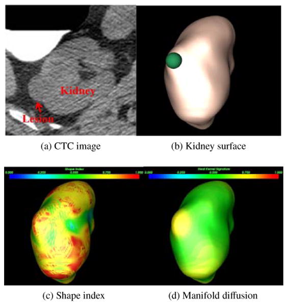
Renal lesion detection on CTC image. (a) A renal lesion located in the right kidney, (b) lesion-caused protuberance on the kidney surface (green sphere), (c) shape index distribution on kidney surface, where blue to red means small to large values, (d) manifold diffusion developed in this paper with increased and differential response on the lesions.

In this work, we develop a novel computer-aided diagnosis system established on two key technologies, efficient belief propagation and intrinsic manifold diffusion. Kidneys are first segmented by embedding probabilistic kidney atlases into an efficient belief propagation framework (Felzenszwalb and Huttenlocher, 2006). An intrinsic manifold diffusion (Liu et al., 2013b) is then computed on the kidney surface to accurately describe geometric transitions (Fig. 1d). Manifold diffusion response has large values in the protuberances (yellow), while suppressed in all other areas (green). Exophytic renal lesions can thus be detected by searching for local maximum diffusion response. Finally, support vector machine is exploited to classify renal lesions using multi-scale diffusion response as shape features, in conjunction with appearance features.

The presented framework extends two preliminary conference papers (Liu et al., 2013a,b), where manifold diffusion with fixed scales were employed to detect ex-ophytic renal lesions and the sum of the Harr wavelet response from speeded up robust features (Bay et al., 2008) were used as appearance features to classify renal lesions. In this work, we investigate the influence of scales on renal lesion detection and incorporate histogram of oriented gradients (Dalal and Triggs, 2005) and local binary pattern (Ojala et al., 1996) as appearance features. We also apply efficient belief propagation to segment pathologic kidneys with renal lesions. Moreover, we extensively evaluate our detection framework on a validation dataset with 167 CTC images containing renal lesions with different sizes and densities.

2. Related Work

This section describes relevant work on kidney segmentation, renal lesion detection and shape analysis.

2.1. Kidney Segmentation

In recent years a large body of research has been conducted on kidney segmentation, the majority focusing on contrast-enhanced CT images (Ali et al., 2007; Khalifa et al., 2011; Lin et al., 2006; Freiman et al., 2010). Probabilistic atlases are often used in kidney segmentation. A set of kidney atlases is first registered to the current patient image. They are then integrated to create the probabilistic atlas. Such integration is meaningful because all registered atlases are referred to the coordinate of the current patient. Exploiting the probabilistic atlas as the shape prior can reduce the segmentation error because the probabilistic atlas represents the possible kidney variability amongst individuals. Ali (Ali et al., 2007) embedded a probabilistic kidney atlas into Markov random fields represented as an energy function. The graph cut algorithm was chosen to minimize the energy function and yield kidney segmentation. Yuksel (Yuksel et al., 2007) extended this work to segment kidneys on dynamic contrast enhanced MRI images by embedding kidney intensity priors into Markov random fields. Similar idea was used in Khalifas approach (Khalifa et al., 2011) by exploiting shape and intensity priors except that a geometric deformable model was used to initialize kidney borders. Another improvement over Ali et al.'s method was the replacement of the parametric kidney atlas with a non-parametric iterative model (Freiman et al., 2010). Lin (Lin et al., 2006) detected kidney candidates by using spine positions as landmarks and searching for elliptic structures. Adaptive region growing algorithm was then employed to segment kidneys on the kidney candidates.

Other researchers treated kidney segmentation within the multi-objects segmentation scheme (Campadelli et al., 2009; Linguraru et al., 2012a), which has the potential to improve the accuracy of kidney segmentation due to the spatial constraints from other organs. Recently, random forest technique (Cuingnet et al., 2012) was applied to kidney segmentation by introducing more comprehensive prior information into the segmentation framework, and a large number of training examples were used to support this process.

However, the majority of the prior methods took advantage of contrast-enhanced CT images and it might be difficult to apply them to non-contrast CTC images. Moreover, shape deformation caused by renal lesions is another issue to hinder accurate kidney segmentation using shape constraints.

2.2. Renal Lesion Detection

In contrast to the large body of research on kidney segmentation, renal lesion detection was seldom addressed. Detection of renal lesions generally consisted of three main steps: kidney segmentation, lesion detection and segmentation. Summers (Summers et al., 2001) developed a marker controlled watershed algorithm to segment both kidneys and lesions. Thresholding algorithm was employed to extract kidneys in (Kim and Park, 2004), and renal lesions were detected and segmented using texture analysis as well as homogeneous region growing. Linguraru (Linguraru et al., 2009) improved renal lesion segmentation by combining fast-matching and geodesic level set. This method generated accurate lesion segmentation, and quantification of renal lesions became feasible. Later on, the lesion type was classified using support vector machine on the lesion segmentation (Linguraru et al., 2011). Landgren (Landgren et al., 2011) used active shape models to extract kidneys in children from scintigraphy images and detected renal lesions based on artificial neural network. Kulamthaivel also investigated neural networks in combination with wavelet-based texture features to classify renal lesions (Kulanthaivel, 2012).

Nevertheless, all these methods investigated texture information of renal lesions because contrast enhancement induces notable intensity difference between lesions and normal kidney tissues. However, texture feature is not distinctive in non-contrast CTC images (Fig. 1a), which makes it difficult to apply these methods to detect renal lesions on CTC images.

2.3. Shape Analysis

Instead of detecting renal lesions in the image domain, we studied shape analysis to resolve this issue in this work. For this reason, we will briefly review shape analysis in computer-aided diagnosis of lesions in this section.

Many lesions are presented as certain geometrical shapes, such as mushroom-like colonic polyps and spherical hepatic tumors. Shape analysis thus plays important roles in detecting lesions and providing meaningful feature descriptors to reduce false positives in computer-aided diagnosis. Curvature was frequently applied to the detection of colonic polyps (Huang et al., 2005; Liu et al., 2011; Sundaram et al., 2007), pulmonary nodules (Kawata et al., 1999) and liver cancer (Linguraru et al., 2012b). An alternative shape analysis tool is shape index (Koenderink and Doorn, 1992), which is a single-value measurement of local surface geometry according to the principal curvature. The local geometry can be classified into cup, rut, saddle, ridge, and cap according to shape index values. This is a useful property for tumor detection in colon (Yoshida et al., 2002), breast (Irishina et al., 2009), and bladder (Li et al., 2008). However, shape index is prone to geometric noise in renal lesion detection (Fig. 1c). The accuracy of shape index might be improved through smoothing organ surface (Desbrun et al., 1999). Surface smoothing is undesirable in renal lesion detection because over-smoothing can cause lesions to vanish.

Recent studies in computer graphics introduced versatile shape descriptors (Bronstein and Kokkinos, 2010; Sun et al., 2008; Litman et al., 2011) based on heat diffusion (Levy, 2006; Reuter et al., 2005). These descriptors are accurate and robust to geometric noise because they smooth while preserving geometric details such as lesions. Because these shape descriptors were established on the heat kernel, constructions related to the heat kernel led to a new research field, called diffusion geometry. Diffusion geometry is intrinsic and deformation-invariant (Levy, 2006), which makes descriptors applicable to deformable shape analysis. In medical image analysis, Seo (Seo et al., 2010) exploited the heat kernel to smooth organ surface, and Lai (Lai et al., 2010) applied this technique to extract geometric features from colon models to perform supine and prone registration.

Our manifold diffusion is also established on the heat kernel. In contrast to the high complexity of the conventional heat kernel diffusion (Seo et al., 2010; Lai et al., 2010), we propose compact, multi-scale heat kernel features for the detection of renal lesions. Although the computation of heat diffusion is simplified, our feature descriptor is still invariant under isometric transformation, as proved in (Sun et al., 2008).

3. Methodology

This section elaborates on our computer-aided detection of exophytic renal lesions (Fig. 2). In this framework, efficient belief propagation method is first chosen to segment left and right kidneys on CTC images. Manifold diffusion is then computed to measure shape variance on the kidney surface. We search for kidney surface regions with local maximum diffusion response as renal lesion candidates. Finally, we established shape and appearance features in the candidate regions and embed them into a support vector machine classifier to determine actual renal lesions and remove false positives.

Figure 2.

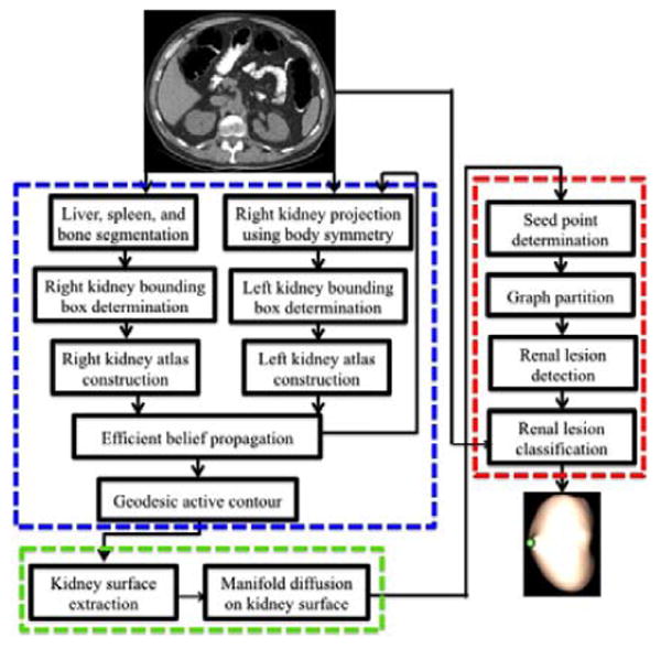
Pipeline of computer-aided detection of exophytic renal lesion, which includes three main components: 1) kidney segmentation (blue frame), 2) manifold diffusion (green), and 3) renal lesion detection and classification (red).

3.1. Kidney Segmentation

An efficient belief propagation approach is developed to segment kidneys on non-contrast CT images for the purpose of limiting the search range of renal lesions. Our method consists of three main components, including data processing, right kidney segmentation, and left kidney segmentation.

3.1.1. Data processing

This step aims to segment liver, spleen and bone to find some anatomical landmarks. These landmarks are used to determine sub-images that envelope the kidneys. Extraction of such sub-images can significantly reduce computational cost as well as improve the accuracy of kidney segmentation. For instance, knowing liver and spleen regions contributes to reduce kidney over-segmentation.

Linguraru's approach (Linguraru et al., 2010) is chosen to segment liver and spleen. Liver and spleen atlases are registered to the patient image followed with 4D convolution and geodesic active contour to improve boundaries of organ registration, which yields the final liver (blue object in Fig. 3a) and spleen (green) segmentations. Bone (red) is segmented by using Yao's method (Yao et al., 2012), in which the spine is segmented and localized via thresholding, region growing, and directed graph searching. The vertebra borders are further refined using a vertebra template. Stemming from the vertebrae, the ribs are then traced by a progressive algorithm based on maximizing the cross-section overlap.

Figure 3.

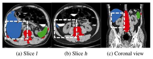
Segmentation of bone (red), liver (blue) and spleen (green) for the determination of sub-images containing the right kidney. (a,b) two slices determined from liver segmentation for the computation of kidney slice range, where white boxes in two axial views illustrate the right kidney spatial range (x-y plane), (c) slice range (z-direction) of the right kidney illustrated by a white box in the coronal view.

3.1.2. Right kidney segmentation

We start with segmenting the right kidney because it is adjacent to the liver and the large volume of the liver facilitates determining a sub-image contain the right kidney. Two key slice indices are first identified from the liver segmentation. One is the slice l with the maximum area of segmented liver (Fig. 3a), and the other one h is the most inferior slice containing the liver (Fig. 3b). The length of a kidney is about 12cm, and it approximately spreads over 120 slices in the CTC images with 1mm slice thickness. Note that the slice h is approximately at the kidney center and the slice l is at one end of the kidney. The slice range of the sub-image is thus defined as [l − 10, h + 60] to ensure that the kidney is included in the sub-image. The length of the white box in Fig. 3c illustrates the slice range of this sub-image. The spatial ranges of the sub-image at x-y image plane are next computed according to the bounding boxes of the liver and bone. Assuming the bounding box of the liver to be [liver_lx, liver_hx, liver_ly, liver_hy, liver_lz, liver_hz] and the bounding box of the bone to be [bone_lx,bone_hx,bone_ly,bone_hy,bone_lz,bone_hz], the sub-image is computed as [bone_lx, (bone_lx + bone_hx)/2, liver_ly, liver_ly + 2/3(liver_hy − liver_ly), l −10,h + 60] (white boxes in Figs. 3a and 3b). We extract a sub-image (Fig. 4a) that mainly contains the right kidney, and threshold it into a binary image (Fig. 4b) by choosing the kidney intensity range of [1, 176]HU as well as removing liver and bone segmentations. Here, the kidney intensity range [1, 176]HU was experimentally determined on our CTC images.

Figure 4.

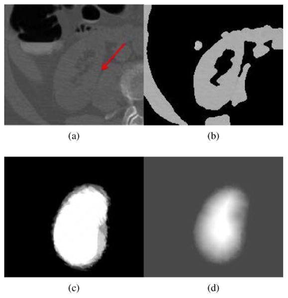
Process of kidney segmentation. (a) Sub-image, (b) binary sub-image after selecting image regions that satisfies kidney intensity values and removing liver and bone regions, (c) probabilistic kidney atlas, and (d) probability field of the right kidney, imported into Eq. 3 to yield kidney segmentation.

Next, we choose five pairs of reference CT images and their right kidney segmentation images to establish a probabilistic kidney atlas. Here, the choice of five reference images is suggested by Rikxoort (van Rikxoort et al., 2010). They performed extensive experiments to demonstrate that five atlases are often sufficient for atlas-based image segmentation, and illustrated their findings in segmenting the heart and the caudate nucleus. The construction of the probabilistic atlas involves four steps. First, we extract five pairs of reference sub-images and their kidney sub-images, and these sub-images have the same size as the ones extracted from the patient image. Second, a reference sub-image and the patient sub-image are registered by affine registration with 9-parameter affine transform (Studholme et al., 1999) and non-rigid registration with a free-form, B-splines deformation (Rueckert et al., 1999). The registration parameters are used to transform the kidney and reference sub-images. Third, affine and non-rigid image registrations are performed again on the binary patient sub-image (Fig. 4b) and the transformed kidney sub-images. The kidney shape variability of different individuals is reduced through the previous two-step image registration, which registers the reference sub-image to the patient sub-image. The transformed kidney sub-image based on registration parameters will be similar to the actual kidney in the patient image. This two-step image registration is performed on all five pairs of reference sub-image and kidney sub-images. Finally, a probabilistic atlas is established by averaging the five registered kidney sub-images (Fig. 4c). The averaging will further reduce registration errors and enable the probabilistic atlas to adapt to the kidney shape of the current patient.

A distance field D(x) (Maurer et al., 2003) is computed on the probabilistic atlas and normalized to [0, 1], which facilitates computing a probability field P(x) of the right kidney. In terms of the kidney intensity I(x) and the normalized distance field D(x), we define the probability field (Fig. 4d) as

$$P(x)=\delta (x)\cdot D(x)$$ (1)

Here, x is an image point and δ(x) is defined as

$$\delta (x)=\{\begin{array}{cc}1& 1<I(x)<176\\ 0& \text{otherwise}\end{array}$$ (2)

where [1, 176]HU is the kidney intensity range.

We formulate the kidney segmentation problem as a labeling process and resort to minimizing an energy function using the Markov random field.

$$E(f_x)=\sum _{x\in \mathrm{\Omega }}min({\Vert P(x)-f_x\Vert }_1,a)+\sum _{y\in N(x)}min(c{\Vert f_y-f_x\Vert }_1,b)$$ (3)

where ‖₁ represents L1 norm, Ω denotes the sub-image domain, N(x) means the neighborhood of x, and 0 ≤ f_x ≤ 1 are labels. In the data term ‖P(x) − f_x‖₁ ∈ [0, 1], we set a = 0.99 to make the data term robust to kidney over-segmentation, which is often caused by the kidney touching surrounding tissues, indicated by a red arrow in Fig. 4a. The truncation value b = 3 is used to prevent the smoothness term ‖f_y−f_x‖₁ from over-smoothing during the labeling process, and the scaling parameter c = 5 is to balance data and smoothness terms in Eq. 3. Here, the constants a, b, and c were selected based on the experimental results in Felzenszwalb's work (Felzenszwalb and Huttenlocher, 2006).

Efficient belief propagation (Felzenszwalb and Huttenlocher, 2006) is chosen to minimize Eq. 3 due to its high efficiency. It is a process of message propagation over the image graph. Each message is a value given by the number of possible f_x. It involves two efficient strategies to reduce the computational cost. First, three-resolution image graphs are built on the patient sub-image. Messages are quickly propagated in the coarse image graph because the local minima of Eq. 3 are rare in the coarse graph. The accuracy of message propagation is improved in the fine image graph. Second, since both terms in Eq. 3 are represented as L1 norm, the belief messages at iteration k can be derived as a nested minimization convolution.

$$m_{x\to y}^k=min(H(f_y),min(H(f_x)+d))$$ (4)

$m_{x\to y}^k$ is the belief message transmitted from x to y at iteration k, d = 1.0, and

$$H(f_x)=\underset{f_x}{min}(min({\Vert P(x)-f_x\Vert }_1,a)+\sum _s{m}_{s\to y}^{k-1})$$ (5)

where s is an image point belonging to six-neighborhood N(y) of y.

Thus, Eq. 3 can be minimized through distance transform (Maurer et al., 2003). The computational time of belief propagation is less than one minute due to these two efficient strategies, and the right kidney is segmented by choosing object points with f_x > 0.05. Here, we set a small threshold 0.05 to ensure exophytic lesions are included because they have small probability values P(x) at the kidney boundary. Finally, geodesic active contour (Caselles et al., 1997) is chosen to smooth right kidney boundaries and recover some missed regions due to large kidney lesions. We initialize zero level set as boundaries of the segmented right kidney from efficient belief propagation, and geodesic active contour forces the level set to propagate towards true right kidney boundaries.

3.1.3. Left kidney segmentation

After the right kidney is segmented, we project it into the left side of the body to determine a sub-image in terms of the body symmetry. We follow the same segmentation strategy to build a probabilistic atlas and perform efficient belief propagation to extract the left kidney. We also use the segmented spleen to reduce the left kidney over-segmentation as well as geodesic active contour to supplement under-segmentation due to large lesions.

Fig. 5 illustrates three examples of kidney segmentation. An endophytic renal lesion is located in the left kidney (Fig. 5a), and our algorithm can accurately segment the kidney (Fig. 5b). A right kidney with an ex-ophytic lesion less than 20mm (Fig. 5c) is also accurately segmented by using our approach (Fig. 5d). The third example is a difficult case because multiple large renal lesions (some larger than 40mm) deform the kidney irregularly (Fig. 5e). However, our method can still segment this pathological case by exploring belief propagation to extract main portion of the kidney regions followed with supplementation using geodesic active contour (Fig. 5f).

Figure 5.

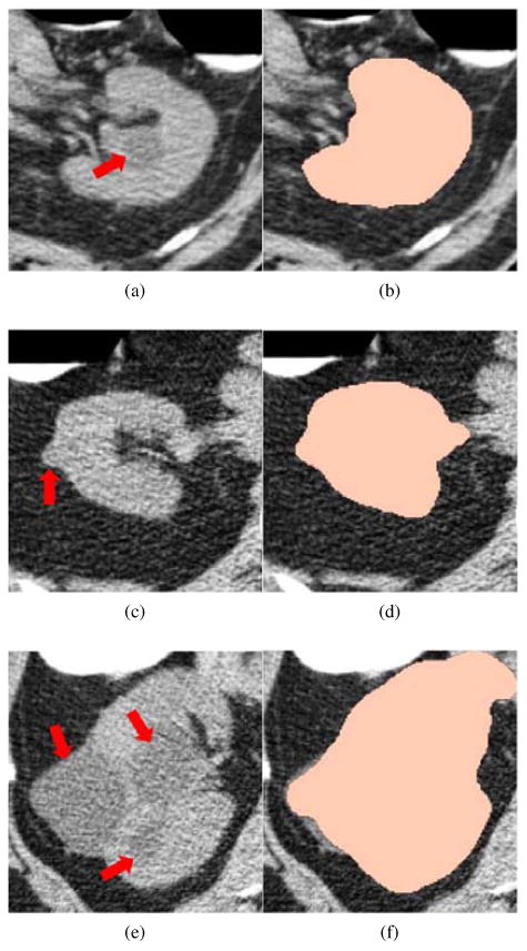
Kidney segmentation on non-contrast CTC images. Left column: Original CTC image where renal lesions are highlighted by red arrows. Right column: corresponding kidney segmentation (peach).

3.2. Manifold Diffusion

After kidneys are segmented, we establish a manifold diffusion process to measure geometric changes on the kidney surface, so as to identify lesion-caused protrusions. The kidney surface is constructed using the Marching Cubes algorithm (Lorensen and Cline, 1987) on the kidney segmentation.

The kidney surface can be generally treated as a three-dimensional complete Riemannian sub-manifold M of ℝ³. Our manifold diffusion on M is governed by the heat equation (Bronstein and Kokkinos, 2010),

$$(\frac{\partial }{\partial t}+{\Delta }_M)U(t,x)=0$$ (6)

where Δ_M is the positive semi-definite Laplace-Beltrami operator on the manifold M and expressed in the parameterization coordinate as (Sun et al., 2008).

$${\Delta }_M=-\frac{1}{\sqrt{det\mathbf{g}}}\sum _{i,j}{\partial }_i\sqrt{det\mathbf{g}{g}_{\mathit{\text{ij}}}^{-1}{\partial }_j}$$ (7)

Here, g is the metric tensor describing the geometric relationship between the manifold M and the parameterization coordinates and det is the determinant of the tensor matrix g. If M has boundaries and F : M → ℝ denotes an initial heat distribution on M, the solution U(t, x) is called the heat distribution at a point x in time t and lim_t→0 U(t, x) = F. For any M, there exists a function K(x, y, t) : ℝ⁺ × ℝ³ × ℝ³ → ℝ (Hsu, 2002), which leads to

$$U(t,x)={\int }_{M}K(x,y,t)F(y)\mathit{\text{dy}}$$ (8)

K(x, y, t) is called the heat kernel and dy is the volume form at y ∈ M, which is a three-dimensional form on the manifold that is nowhere equal to zero. K(x, y, t) measures the amounts of the heat transferred from x to y at time t.

According to graph spectral theory (Chung, 1996), K(x, y, t) is decomposed as

$$K(x,y,t)=\sum _{i\ge 0}{e}^{-{\lambda }_{i}t}{\varphi }_i(x){\varphi }_i(y)$$ (9)

Here, λ_i and ϕ_i are, respectively, the ith eigenvalue and the ith eigenfunction of the Laplace-Beltrami operator. The parameter t takes the scale role in shape analysis because adjusting it can produce a family of K(x, y, t). Setting x = y, K(x, y, t) is referred to as the auto-diffusivity function, which denotes the amount of heat remaining at a point x after time t. Our manifold diffusion is defined according to K(x, x, t) by varying the scale t (Fig. 6).

Figure 6.

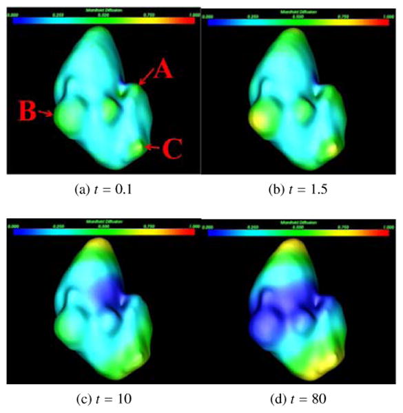
Manifold diffusion at different scales. Three renal lesions are marked as A, B, and C in (a), which are used to illustrate the influence of manifold diffusion on their detection.

Manifold diffusion at small scales can accurately detect lesion-caused protrusions because it is correlated with Gaussian curvature S (x) (Sun et al., 2008) as

$$K(x,y,t)\approx \frac{1}{4{\pi }^2}(1+\frac{1}{6}S(x)t+O(x,t^2))$$ (10)

where O(x, t²) is the higher-order term of x and t. Manifold diffusion is superior to Gaussian curvature as the diffusion process also eliminates geometrical noise and yields smooth shape measurements over the kidney surface. For instance, a small lesion A (Fig. 6a) can be stably detected when t = 0.1 because its diffusion response is locally maximum (mapped in green) in comparison with its neighboring points (cyan). Large lesions B and C are easily detected when t = 1.5 because their responses are more dominant at this scale (Fig. 6b). The kidney surfaces with large diffusion response are gradually shifted to the superior and inferior kidney segments as they are two most stable protrusions (Fig. 6d). Therefore, our manifold diffusion at small scales is a good fit for renal lesion detection.

Shape descriptors based on the manifold diffusion also provide several beneficial properties for the classification of renal lesions. First, the Laplace-Beltrami operator is intrinsically defined on M, and the feature descriptor established on this operator is invariant under isometric transformation (Bronstein and Kokkinos, 2010; Sun et al., 2008). In other words, our feature descriptor is insensitive to the variability among renal lesions. Second, the collection of manifold diffusion responses at different scales is a compact shape descriptor that can densely measure shape variance on the kidney surface. Third, the feature descriptor is informative, as it keeps all information about the intrinsic geometry of the manifold (Sun et al., 2008). Lastly, the feature descriptor from manifold diffusion accurately preserves all local shape information because it is established on the kidney surfaces with original resolutions.

3.3. Renal Lesion Detection and Classification

Manifold diffusion response computed from the previous step is assigned as the vertex weight of the kidney surface graph because the kidney surface extracted from the Marching Cubes algorithm is naturally a graph representation. Renal lesions are highlighted at small scales (Figs. 6a and 6b), and we choose a set of fine scales to allow for our framework to identify renal lesions with different sizes. In our implementation, we use t ∈ [0.1, 0.5, 1.0, 1.5, 2.0] in Eq. 9. The kidney graph is then partitioned to search for sub-graphs with local maximum scale response, as renal lesions typically stay in these regions. Fig. 7 summarizes the process of our renal lesion detection, which consists of four main steps, including seed point determination, graph partition, renal lesion detection, and lesion classification.

Figure 7.

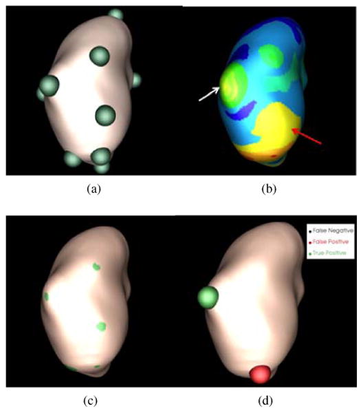
Process of renal lesion detection on a CTC image in Fig. 1a. (a) Seed point determination, (b) graph partition, (c) renal lesion detection, and (d) lesion classification.

3.3.1. Seed point determination

This step searches for a set of vertices with local maximum diffusion response at each predefined, small scale. They are used as seed points to facilitate partitioning kidney surface graphs. A seed point x_s is determined if K(x_s, x_s, t) = arg max _x∈ring(5) K(x, x, t), where ring means the neighbors of x on the surface graph (Desbrun et al., 1999). A small number of rings will select a large number of seed points with local maximum response values which will increase computational cost in the graph partition step. On the other hand, a large number of rings will increase the computational time of searching for seed points. We ran the experiments using 2-11 rings to search for seed points, and found that five rings optimally balanced the computational cost and accuracy of seed point determination. Green spheres in Fig. 7a illustrate the detected seed points.

3.3.2. Graph Partition

The normalized cut algorithm (Shi and Malik, 2000) is employed to partition the kidney surface graph. Let G = (E, V) be the kidney surface graph with the edge set E and the vertex set V. The edge weight is assigned with the sum of diffusion response difference across predefined scales,

$$W(x_1,x_2)={\left({\int }_{0.1}^2{(K(x_1,x_1,t)-K(x_2,x_2,t))}^2\mathit{\text{dt}}\right)}^{1/2},(x_1,x_2)\in E$$ (11)

Here, we define the interval [0.1, 2] because we choose these scales to detect renal lesions.

A cut is define as

$$\mathit{\text{cut}}(A,B)=\sum _{x_1\in A,x_2\in B}W(x_1,x_2)$$ (12)

which is to find a set of edges to separate G into two disjoint sets A and B with similar diffusion response values measured by Eq. 11. Normalized cut is computed as

$$N\mathit{\text{cut}}(A,B)=\frac{\mathit{\text{cut}}(A,B)}{\mathit{\text{assoc}}(A,V)}+\frac{\mathit{\text{cut}}(A,B)}{\mathit{\text{assoc}}(B,V)}$$ (13)

where assoc(A, V) = Σ_{x1∈A,x2∈V} W(x₁,x₂) and assoc(B,V) is similarly defined. Normalized cut is iteratively performed until no graph partitions contain two seed points and the deviation of diffusion values of each partition is also less than 0.1. Fig. 7b shows the partition results where each partition is represented as a colored component.

3.3.3. Renal Lesion Detection

A partition is regarded as a lesion candidate if its diffusion response is the local maximum and its area is less than a threshold, α =1cm². α is used to distinguish image partitions with local maxima, such as the two partitions indicated by arrows in Fig. 7b. The partition indicated by the red arrow belongs to the normal kidney surface and it has a large surface area. The partition indicated by the white arrow (an exophytic lesion) has a small area. 1cm² is experimentally determined from the training dataset based on the observation in Fig. 7b that the partition includes parts of the lesion surface has the limited size. In other words, most of the partitions with renal lesions are less than 1cm². Fig. 7c illustrates the graph partitions in green regions belonging to lesion candidates.

3.3.4. Lesion classification

For classification, we map the center point of the lesion candidates to the original CT image. A 10×10×10 sub-image centered at the mapped point is constructed for computing appearance features. Mean and standard deviation of intensity values, local binary pattern (Ojala et al., 1996), histogram of oriented gradients (Dalal and Triggs, 2005), as well as speeded up robust features (Bay et al., 2008) are used to describe the lesion appearance. Multi-scale manifold diffusion response is used to characterize the lesion shape. Table 1 gives the dimensions of all texture features and shape features for lesion classification. We combine appearance and shape information to formulate feature vectors. LBP, HOG and SURF measure the texture response in different orientations, and the combination of all orientations can accurately describe the texture characteristic in the current lesion candidate. Our early work (Wang et al., 2012; Liu et al., 2013c) showed that using all features could achieve similar detection accuracy to using feature subsets determined using feature selection and dimension reduction. Thus, we applied all feature vectors to train the support vector machine classifier (Chang and Lin, 2011) using a Gaussian radial basis function as the kernel. The final lesion detection after classification is shown in Fig. 7d. Here, the green sphere represents true positive and the red one false positive.

Table 1.

Dimensions of texture features and shape features for lesion classification.

Features	LBP	HOG	SURF	MMD
Dimensions	64	124	48	101

4. Validation Datasets and Methods

Our lab has collected 1186 non-contrast CTC images from three institutions (Pickhardt et al., 2003). Each dataset was scanned during a single breath hold using a four-channel or eight-channel CT scanner (General Electric Light Speed or Light Speed Ultra, GE Healthcare Technologies, Waukesha, WI). CT scanning parameters included 1.25 to 2.5 mm section collimation, 15 mm table speed, 1 mm reconstruction interval, 100 mAs, and 120 kVp. Retrospective analysis of these images was approved by our Office of Human Subject Research. With the assistance of an experienced radiologist, 97 patients were confirmed to have renal lesions based on clinical reports from three institutions providing CTC data. 76 of patients with renal lesions contained exophytic lesions. We excluded one patient with an exceptionally large kidney lesion (125. 12mm) leaving 96 patients with renal lesions. 71 patients without lesions from the remaining CTC images were also included. Thus, 167 CTC images (patient age range, 43-73 years; mean age, 56±8 years) compose the validation dataset to evaluate our renal lesion detection framework.

The total number of lesions from the 96 patients was 179. 141 of them were exophytic, and the remaining 38 were endophytic. All lesions were marked by an experienced radiologist as the groundtruth. The lesion size range was 0.3-6.6cm and mean size was 2±1.4cm. The lesion CT attenuation ranged from -313-40HU with a mean of 2±32HU. The number of left kidney surface points reconstructed by the Marching Cubes algorithm was 33684-113492 (mean point number, 55062±13178), and the number of right kidney surface points was 34536-98600 (mean point number, 54556±12171).

We evenly divided the 167 patients into five folds and performed five-fold cross-validation. The first three folds have 33 patients and the remaining two have 34. Because we focus on the detection of exophytic renal lesions in this work, we also evenly assigned 76 patients with exophytic lesions into 5 folds. The first four folds had 15 patients with exophytic lesions and the last fold had 16. Table 2 gives the detailed information about the numbers of patients and lesions in each fold.

Table 2.

Numbercients with exophytic lesions (Pati/Ex), exophytic lesions (Ex) and endophytic lesions (En) in five folds.

Fold	No. 1	No. 2	No. 3	No. 4	No. 5
# of Pati	33	33	33	34	34
# of Pati/Ex	15	15	15	15	16
# of Ex	34	33	27	22	25
# of En	8	10	15	4	1

We designed another configuration of training and testing dataset to measure the influence of diffusion scale selection, lesion size, lesion density, and lesion type on the detection accuracy. We randomly selected the second and the fourth folds to formulate the training dataset (67 patients), and the remaining three folds as the testing dataset (100 patients). Increasing the number of patients in the testing dataset contributes to better analyze different parameter choice on the detection accuracy. There were 30 patients with exophytic renal lesions in the training dataset, and 46 patients in the testing dataset. In the training dataset, the total number of exophytic renal lesions was 56. In the testing dataset, the number of exophytic renal lesions was 85.

We first performed five-fold cross-validation to analyze the stability of computer-aided exophytic renal lesion detection. We then chose the testing dataset with three folds to evaluate the choice of diffusion scale in exophytic lesion detection by comparing detection results using multi-scales (t=0.1, 0.5, 1.0, 1.5, and 2.0), and each individual scale. Here, renal lesion detection was considered as true positive if the distance between the detection and the reference is less than half of the corresponding lesion size as well as the detected point being located within the renal lesion. Otherwise, it was called false positive. The free-response receiver operating characteristic (FROC) analysis (Hillis et al., 2009) is chosen to evaluate the accuracy of renal lesion detection.

We also compared multi-scale manifold diffusion with the conventional shape features including shape index, minimum curvature, maximum curvature, Gaussian curvature, and mean curvature, to better understand the advantages of manifold diffusion on exophytic renal lesion detection. We imported conventional shape features into the same pipeline of renal lesion detection and classification in section 3.3. Because conventional shape features produced a large number of seed points, we merged seed points if their distance is less than 1cm to ensure the normalized-cut method stably partition kidney surface.

Lesion size and density are two important features that describe the lesion shape and appearance, and we thus also analyzed detection accuracy as a function of the renal size as well as a function of the lesion density to evaluate their influence. Finally, we reported the detection accuracy of exophytic and endophytic lesions.

5. Experimental Results

In this section, we report the accuracy of renal lesion detection on the validation dataset.

5.1. Five-fold cross-validation

In Fig. 8, we compared the performance of the proposed method using five-fold cross-validation. The detection accuracy achieved 95% sensitivity at 12 false positives per patient on all five folds except the third fold. The false positives increased to 19 to achieve 95% sensitivity. The performance was lower in the third fold because 89% (24/27) of exophytic lesions in this fold were less than 2cm compared to less than 57% in the other four folds. Moreover, inaccurate kidney segmentations contained many protrusions due to large levels of image noise in some CTC images. Such protrusions were similar to the exophytic lesions and caused 34% more initial detections than the other four folds.

Figure 8.

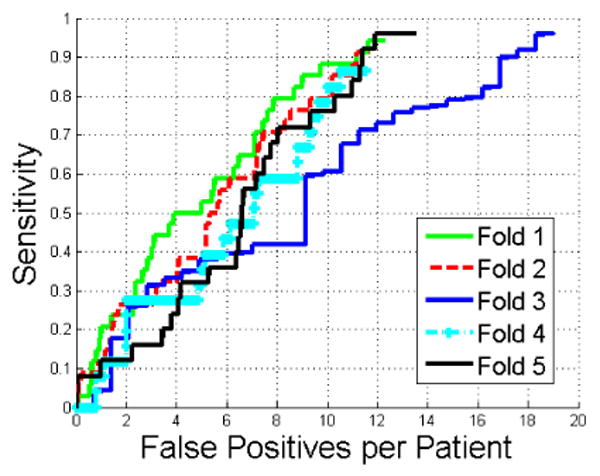
Comparison of FROC curves of renal lesion detection in five-fold cross-validation.

5.2. Scale selection of manifold diffusion

Fig. 9 compares the detection accuracy of exophytic lesions using multi-scale manifold diffusion and single-scale manifold diffusion at different scales. Manifold diffusion at a single scale is inappropriate for lesion detection because it missed many renal lesions. The highest sensitivity is 70% with 15 false positives per patient (cyan curve) at t=1. In contrast, multi-scale manifold diffusion is superior to single-scale manifold diffusion because it achieves 95% sensitivity at 15 false positives per patient.

Figure 9.

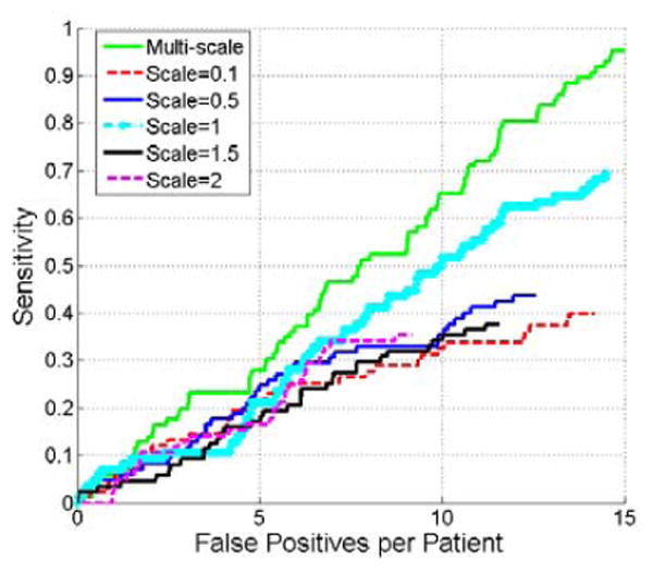
Comparison of FROC curves of renal lesion detection using multi-scale manifold diffusion and single-scale manifold diffusion at t=0.1, 0.5, 1, 1.5, and 2.

Fig. 10 shows renal lesion detection on the right kidney using multi-scale manifold diffusion. Single scales t=0.5 and t=2 can detect lesions with small and large perturbations, respectively, in Figs. 10b and 10c. In contrast, multi-scale manifold diffusion can find both lesions (Fig. 10d).

Figure 10.

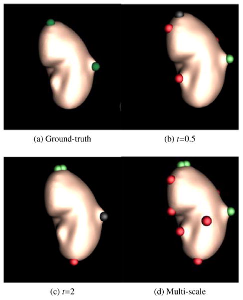
Multi-scale effects of manifold diffusion on renal lesion detection. A small scale t=0.5 accurately detected a renal lesion (green sphere) with small perturbation in (b), while it missed the lesion (black sphere) on the top of kidney with large perturbation. On the contrary, a large scale t=2 found the lesion on the top while missed the lesion in the right in (c). Multi-scale manifold diffusion addresses these issues by combining detection results from a set of scales in (d).

5.3. Comparison of manifold diffusion with conventional shape features

This section compares detection results from manifold diffusion with those from conventional shape features, including shape index, Gaussian curvature, mean curvature, minimum curvature, and maximum curvature. Fig. 11 indicates that manifold diffusion significantly outperform conventional shape features because at 15 false positives their sensitivities are all less than 50% while our manifold diffusion achieves 95% (p < 1e −r 3 reported by JAFROC (Chakraborty, 2006)).

Figure 11.

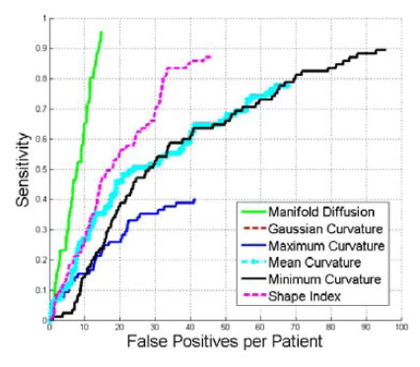
Comparison of FROC curves of renal lesion detection using multi-scale manifold diffusion, Gaussian curvature, maximum curvature, mean curvature, minimum curvature, and shape index. Multi-scale manifold diffusion significantly outperforms all other shape descriptors in renal lesion detection (p < 1e − 3).

5.4. Influence of lesion sizes on the detection accuracy

This section evaluates the influence of lesion size on the detection accuracy. Fig. 12 gives the detection results on the lesions with different sizes. Our method tends to achieve high detection accuracy on larger renal lesions (30 mm or larger) and comparable accuracy on lesions less than 20mm.

Figure 12.

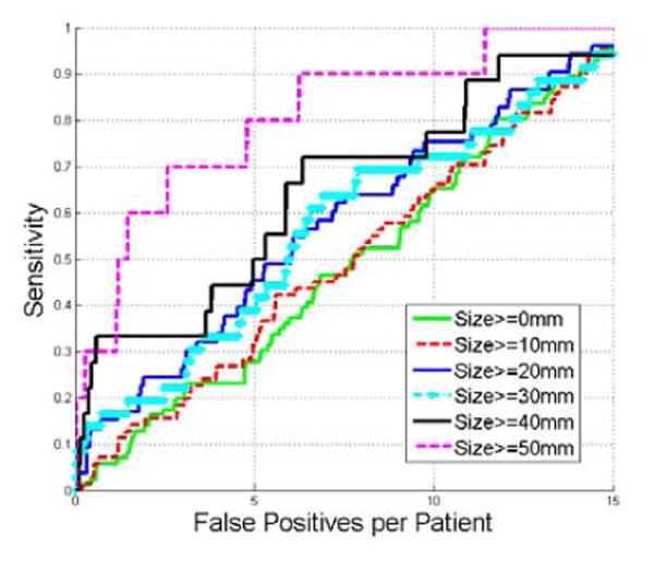
Comparison of FROC curves of detecting renal lesions with different sizes.

5.5. Influence of lesion densities on the detection accuracy

In this section, we analyze the effect of renal lesion densities on the detection accuracy. We can observe that Fig. 13 is similar to Fig. 12. Renal lesions with higher density (≥30 HU) have higher detection accuracy.

Figure 13.

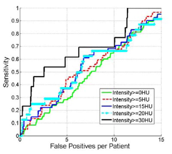
Comparison of FROC curves of detecting renal lesions with different densities.

5.6. Detection accuracy of exophytic and endophytic lesions

We also tested manifold diffusion method on endophytic renal lesions, and the detection accuracy of ex-ophytic and endophytic renal lesions are reported in Fig. 14. At 15 false positives, the sensitivity of exophytic lesion detection is 95% while it is 80% on the endophytic lesion detection. This result is not surprising because manifold diffusion attempts to find lesion-caused protuberance on the kidney surface while endophytic lesions produce little deformations, such as for lesion A (Fig. 15a). The lack of surface protrusions prevents our manifold diffusion method from detecting it (Black sphere in Fig. 15b). However, manifold diffusion can detect endophytic lesions near the kidney hilum (lesion B in Fig. 15c), because the concave hilum has strong diffusion response.

Figure 14.

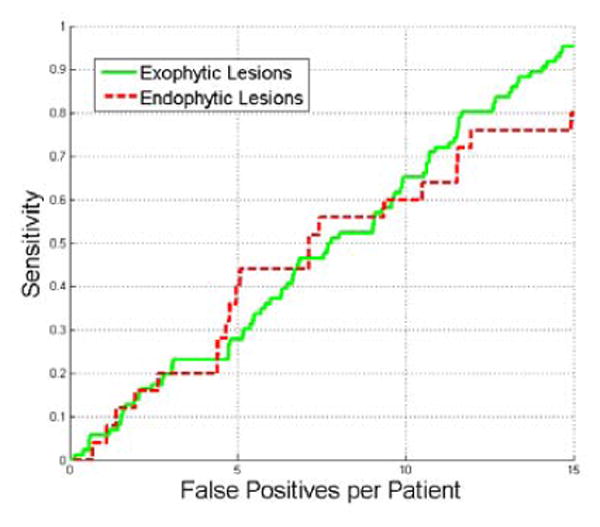
Comparison of FROC curves of detection accuracy on ex-ophytic and endophytic lesions.

Figure 15.

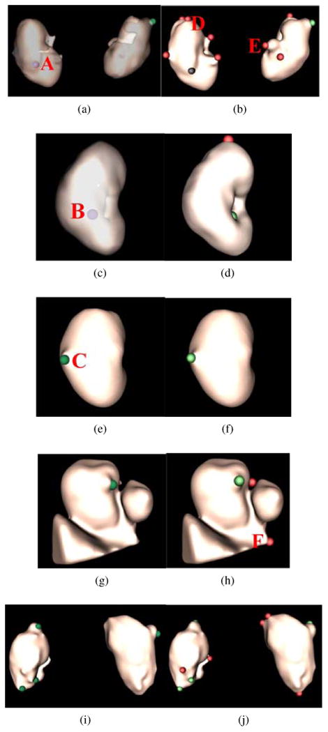
Renal lesion detection on five patient datasets corresponding to five rows. Renal lesion annotations are illustrated in the left column where exophytic lesions are in red and internal lesions in violet. To better observe internal lesions A and B, the kidney surface is transparently visualized in (a) and (c). Lesion detections are presented in the right column, where true positives are in green, false positives in red, and false negatives in black.

As for exophytic lesions, our method can reliably identify them. Lesion C is a typical example (Fig. 15e), and manifold diffusion can find it without false positives (Fig. 15f). Manifold diffusion is also robust to inaccurate kidney segmentation (Fig. 15g). Kidney segmentation erroneously contains part of the liver (triangular object) and the inferior vena cava (round blob). An ex-ophytic lesion is still detected by using manifold diffusion (Fig. 15h). The patient in the last row contains four exophytic lesions, and our method can detect all of them.

32% of false positives were located in the superior and inferior kidney (detection D in Fig. 15b); 35% near the kidney hilum because kidney segmentation includes part of the vein or artery, which caused protrusions in the kidney segmentation (detection E in Fig. 15b); the remaining 23% of false positives are due to kidney over-segmentation, such as liver tissue (detection F in Fig. 15h). Nevertheless, improvement of kidney segmentation will be desirable to reduce the number of false positives.

6. Discussion

In this work, we developed a computer-aided diagnosis system to detect exophytic renal lesions on non-contrast CTC images using efficient belief propagation and manifold diffusion. Efficient belief propagation successfully segmented kidneys on patients with and without renal lesions by embedding a probabilistic kidney atlas from five reference CT images and their kidney segmentation. Segmentation results on 167 patients confirmed that the probabilistic atlas from five reference images was stable to kidney variability. The segmentation results also demonstrated that the efficient belief propagation method was robust to some characteristics of CT colonography, such as insufflation of the bowel with carbon dioxide.

After kidneys were segmented, a manifold diffusion process was established on the kidney surface based on the Riemannian geometry because non-contrast CTC images lack visual cues. Manifold diffusion instead smoothly and accurately measured shape changes on the kidney surface, so as to identify lesion-caused protuberances with local maximum diffusion response. Moreover, diffusion response was employed as shape features to classify renal lesions and reduce false positives. The diffusion response in Fig. 6 indicated that fine-scale response was sensitive to small surface protuberances, potentially caused by renal lesions, while coarse-scale responses tend to be stable at large protuberance, such as the superior tip of the kidney. Thus, fine-scale manifold diffusion was chosen to detect renal lesions. Figs. 9 and 10 also revealed that diffusion response with a set of small scales generated the most accurate detections in comparison with different single scales because renal lesions with different sizes demands multi-scale manifold diffusion. For this reason, multi-scale manifold diffusion was used to detect exophytic lesions in this work. Five-fold cross-validation also proved that manifold diffusion could stably detect renal lesions.

We compared multi-scale manifold diffusion with some conventional shape features including shape index, Gaussian curvature, mean curvature, minimum curvature, and maximum curvature. Manifold diffusion significantly outperforms conventional shape features because at 15 false positives their sensitivities are all less than 50% while manifold diffusion achieves 95% (p < 1e−3). Manifold diffusion globally creates smooth and accurate shape measurements on the kidney surface. It can accurately identify lesion-caused protuberances while eliminating geometrical noise. On the contrary, conventional shape features are single-scalar measurements, which highly depend on local geometry. These measurements are sensitive to geometrical noise, which yields many false positives. Meanwhile, conventional shape features, such as shape index in Fig. 1c, often cause kidney surface graph to be over-segmented. Large graph partition fails to fulfill the condition that the area of the partition should be less than a threshold α=1cm², defined in the section of renal lesion detection. Thus, conventional shape features also miss many renal lesions. Here, the threshold α and some other parameters in our computer-aided diagnosis system were experimentally determined in the training dataset. The validation results on the test dataset demonstrated that the choice of these parameters can achieve accurate renal lesion detection.

Experimental results in Fig. 12 show that the detection accuracy is highly correlated with the lesion size as detection on large lesions achieves high sensitivity with few false positives. This result is anticipated because large lesions tend to cause large protuberances on the kidney surface. Correspondingly, manifold diffusion response is strong on the kidney surface, which facilitates our framework to detect them. Therefore, lesion size has a significant impact on the renal lesion detection. A similar finding is observed in Fig 13, where the detection accuracy is dependent on lesion densities, and renal lesions with high densities are more easily detected than those with small densities. This property might be useful for subsequent tasks that further characterize lesion types.

We also analyze the detection accuracy of endophytic and exophytic lesions. At 15 false positives, the sensitivity of exophytic lesion detection is 95% while it is 80% on the endophytic lesion detection. This result is not surprising because some internal renal lesions do not cause the kidney surface to deform (Fig. 15a) and manifold diffusion fails to find them. However, manifold diffusion can still detect lesions in the kidney hilum where there is a strong diffusion response. Almost all exophytic lesions are accurately detected even in the case of inaccurate kidney segmentation (Fig. 15g) because manifold diffusion can identify their corresponding protuberances. The superior and inferior tips of the kidneys, the renal artery and vein, and inaccurate kidney segmentation are three primary factors that produce false positives.

The method we have presented may have important clinical utility for CT colonography image interpretation. Extracolonic findings are an important aspect of CTC image interpretation. Extracolonic findings must be detected and occasionally will lead to additional imaging or even surgery. The kidneys are the primary source of extracolonic findings on CTC scans (Yee et al., 2005). Multi-scale manifold diffusion can achieve 95% detection accuracy of exophytic renal lesions with only 15 false positives per patient. Based on the discussion with radiologists in our institute, they can quickly distinguish true detections from false positives. To the best of our knowledge, manifold diffusion is the first method applied for the detection of renal lesions on non-contrast CT images. Even in comparison with the detection accuracy on contrast-enhanced CT images (96% sensitivity with 6 false positive per patients (Landgren et al., 2011) on a validation dataset with 40 patients), our method is still comparable considering the challenges of non-intravenous contrast-enhanced CT colonography images.

In the future, we will investigate three important issues to improve the detect accuracy as well as reduce false positives. First, we are studying Gaussian scale space theory (Lindeberg, 1994) to develop a metric to automatically select manifold diffusion scale t, instead of assigning it with a set of fixed scales from [0.1, 2] in Eq. 11. The number of false positives might be reduced because selected diffusion scales are directly correlated with different lesions. Second, we are exploring multi-organ segmentation (Linguraru et al., 2012a) to remove more organs adjacent to kidneys. The elimination of more organs can reduce the size of sub-image used in the kidney segmentation and improve the final segmentation. Accurate kidney segmentation not only enhances the detection accuracy, but also reduces false positives. The last important issue is the detection of endophytic lesions not adjacent to the kidney hilum, such as lesion A in Fig. 15a. Based on our observation, these lesions tend to present spherical shapes inside the kidney and also have slightly lower intensity values than their surround kidney tissues. We are exploring these two characteristics to extend our detection system to find such internal lesions by constructing multi-scale endophytic lesion atlases.

Highlights.

• We developed a novel computer-aided diagnosis system to detect renal lesions on non-contrast CT images.

• We designed an efficient belief propagation method to accurately segment kidneys on non-contrast CT images.

• A novel shape descriptor, manifold diffusion, was presented in this work. It was compact, isometric invariant, and it can accurately and smoothly measure shape changes on the kidney surface.

• We devised a novel renal lesion detection metric by assigning diffusion response as the weight of kidney surface graph, exploring normalized-cut algorithm to partition kidney surface graph, and detecting renal lesions with local maximum diffusion response.

• We extensively validated the proposed method on a large dataset with 167 patients, and experimental results demonstrated that our manifold diffusion method could achieve 95% sensitivity with 15 false positives per patient. We also proved that manifold diffusion significantly outperformed conventional shape descriptors, such as shape index (p<1e-3).

References

- Ali A, Farag A, El-baz A. Graph cuts framework for kidney segmentation with prior shape constraints. Proceedings of the International conference on Medical Image Computing and Computer-Assisted Intervention. 2007:384–392. doi: 10.1007/978-3-540-75757-3_47. [DOI] [PubMed] [Google Scholar]
- Bay H, Ess A, Tuytelaars T, Gool L. Surf: Speeded up robust features. Computer Vision and Image Understanding. 2008;110:346–359. [Google Scholar]
- Bronstein M, Kokkinos I. Scale-invariant heat kernel signatures for non-rigid shape recognition. Proceedings of the IEEE Conference on Computer Vision and Pattern Recognition. 2010:1704–1711. [Google Scholar]
- Campadelli P, Casiraghi E, Pratissoli S, Lombardi G. Automatic abdominal organ segmentation from ct images. Electronic Letters on Computer Vision and Image Analysis. 2009;8:1–14. [Google Scholar]
- Caselles V, Kimmel R, Sapiro G. Geodesic active contours. Intrernational Journal of Computer Vision. 1997;22:61–79. [Google Scholar]
- Chakraborty D. Analysis of location specific observer performance data: validated extensions of the jackknife free-response (jafroc) method. Academic Radiology. 2006;13:1187–1193. doi: 10.1016/j.acra.2006.06.016. [DOI] [PubMed] [Google Scholar]
- Chang C, Lin C. Libsvm: A library for support vector machines. ACM Transactions on Intelligent Systems and Technology. 2011;2:1–27. [Google Scholar]
- Chung F. Spectral Graph Theory (CBMS Regional Conference Series in Mathematics, No. 92) American Mathematical Society; 1996. [Google Scholar]
- Cootes T, Taylor C, Cooper D, Graham J. Active shape models - their training and application. Computer Vision and Image Understanding. 1995;61:38–59. [Google Scholar]
- Cuingnet R, Prevost R, Lesage D, Cohen L, Mory B, Ardon R. Automatic detection and segmentation of kidneys in 3d ct images using random forests. Proceedings of the International conference on Medical Image Computing and Computer-Assisted Intervention. 2012:66–74. doi: 10.1007/978-3-642-33454-2_9. [DOI] [PubMed] [Google Scholar]
- Dachman A, Obuchowski N, Hoffmeister J, Hinshaw JL, Frew M, Winter T, Uitert RV, Periaswamy S, Summers R, Hill-man BJ. Effect of computer-aided detection for ct colonography in a multireader, multicase trial. Radiology. 2010;256:827–835. doi: 10.1148/radiol.10091890. [DOI] [PMC free article] [PubMed] [Google Scholar]
- Dalal N, Triggs B. Histograms of oriented gradients for human detection. Proc. of IEEE Conference on Computer Vision and Pattern Recognition. 2005:886–893. [Google Scholar]
- Desbrun M, Meyer M, Schroder P, Barr AH. Implicit fairing of irregular meshes using diffusion and curvature flow. Computer Graphics. 1999;33:317–324. [Google Scholar]
- Felzenszwalb P, Huttenlocher D. Efficient belief propagation for early vision. International Journal of Computer Vision. 2006;70:41–54. [Google Scholar]
- Freiman A, Esses S, Joskowicz L, Sosna J. Non-parametric iterative model constraint graph min-cut for automatic kidney segmentation. Proceedings of the International conference on Medical Image Computing and Computer-Assisted Intervention. 2010:73–80. doi: 10.1007/978-3-642-15711-0_10. [DOI] [PubMed] [Google Scholar]
- Hillis S, Berbaum K, Metz C. Recent developments in the dorfman-berbaum-metz procedure for multireader roc study analysis. Academic Radiology. 2009;15:647–661. doi: 10.1016/j.acra.2007.12.015. [DOI] [PMC free article] [PubMed] [Google Scholar]
- Homma Y, Kawabe K, Kitamura T, Nishimura Y, Shinohara M, Kondo Y, Saito I, Minowada S, Asakage Y. Increased incidental detection and reduced mortality in renal cancer–recent retrospective analysis at eight institutions. International journal of urology. 1995;2:77–80. doi: 10.1111/j.1442-2042.1995.tb00428.x. [DOI] [PubMed] [Google Scholar]
- Hsu E. Stochastic Analysis on Manifolds. American Mathematical Society 2002 [Google Scholar]
- Huang A, Summers R, Hara A. Surface curvature estimation for automatic colonic polyp detection. Proceedings of the SPIE Medical Imaging: Physiology, Function, and Structure from Medical Images 2005 [Google Scholar]
- Irishina N, Moscoso M, Dorn O. Microwave imaging for early breast cancer detection using a shape-based strategy. IEEE Transactions on Biomedical Engineering. 2009;56:1143–1153. doi: 10.1109/TBME.2009.2012398. [DOI] [PubMed] [Google Scholar]
- Jayson M, Sanders H. Increased incidence of serendipitously discovered renal cell carcinoma. Urology. 1998;51:203–205. doi: 10.1016/s0090-4295(97)00506-2. [DOI] [PubMed] [Google Scholar]
- Kawata Y, Niki N, Ohmatsu H, Kakinuma R, Mori K, Eguchi K, Kaneko M, Moriyama N, Kusumoto M, Nishiyama H. Computer aided differential diagnosis of pulmonary nodules using curvature based analysis. Proceedings of the 10th International Conference on Image Analysis and Processing. 1999:470–475. [Google Scholar]
- Khalifa F, Elnakib A, Beache G, Gimelfarb G, ElGhar M, Quseph R, Sokhadze G, Manning S, McClure P, El-Baz A. 3d kidney segmentation from ct images using a level set approach guided by a novel stochastic speed function. Proceedings of the International conference on Medical Image Computing and Computer-Assisted Intervention. 2011:587–594. doi: 10.1007/978-3-642-23626-6_72. [DOI] [PubMed] [Google Scholar]
- Kim D, Park J. Computer-aided detection of kidney tumor on abdominal computed tomography scans. Acta radiologica. 2004;45:791–795. doi: 10.1080/02841850410001312. [DOI] [PubMed] [Google Scholar]
- Kimberly J, Phillips K, Santago P, Perumpillichira J, Bechtold R, Pineau B, Vining D, Bloomfeld R. Extracolonic findings at virtual colonoscopy: an important consideration in asymptomatic colorectal cancer screening. Journal of general internal medicine. 2009;24:69–73. doi: 10.1007/s11606-008-0835-2. [DOI] [PMC free article] [PubMed] [Google Scholar]
- Koenderink J, Doorn A. Surface shape and curvature scales. Image and Vision Computing. 1992;10:557–564. [Google Scholar]
- Kulanthaivel G. Proc. of International Conference on Emerging Trends in Computer and Electronics Engineering. Dubai: 2012. Diagnostic classification of renal lesions using wavelet based texture descriptors in web environment. [Google Scholar]
- Lai Z, Hu J, Liu C, Taimour V, Pai D, Zhu J, Xu J, Hua J. Intra-patient supine-prone colon registration in ct colonography using shape spectrum. Proceedings of the International conference on Medical Image Computing and Computer-Assisted Intervention. 2010:332–339. doi: 10.1007/978-3-642-15705-9_41. [DOI] [PubMed] [Google Scholar]
- Landgren M, Sjostrand K, Ohlsson M, Stahl D, Overgaard N, Astrom K, Sixt R, Edenbrandt L. An automated system for the detection and diagnosis of kidney lesions in children from scintigraphy images. Proceedings of the the 17th Scandinavian conference on Image analysis. 2011:489–500. [Google Scholar]
- Lee C, Katz J, Fearn P, Russo P. Mode of presentation of renal cell carcinoma provides prognostic information. Urologic oncology. 2002;7:135–140. doi: 10.1016/s1078-1439(01)00185-5. [DOI] [PubMed] [Google Scholar]
- Levy B. Laplace-beltrami eigenfunctions towards an algorithm that understands geometry. Proc. of the IEEE International Conference on Shape Modeling and Applications 2006 [Google Scholar]
- Li L, Wang Z, Liang Z. Cancer Models with Applications (Series in Mathematic Biology and Medicine) World Scientific Publishing; 2008. Bladder cancer screening by magnetic resonance imaging; pp. 457–469. [Google Scholar]
- Lin D, Lei C, Hung S. Computer-aided kidney segmentation on abdominal ct images. IEEE Transactions on Information Technology in Biomedicine. 2006;10:59–65. doi: 10.1109/titb.2005.855561. [DOI] [PubMed] [Google Scholar]
- Lindeberg T. Scale-Space Theory in Computer Vision. Kluwer Academic Publishers; 1994. [Google Scholar]
- Linguraru M, Pura J, Pamulapati V, Summers R. Statistical 4d graphs for multi-organ segmentation from multi-phase abdominal ct. Medical Image Analysis. 2012a;16:904–914. doi: 10.1016/j.media.2012.02.001. [DOI] [PMC free article] [PubMed] [Google Scholar]
- Linguraru M, Richbourg W, Liu J, Watt J, Pamulapati V, Wang S, Summers R. Tumor burden analysis on computed tomography by automated liver and tumor segmentation. IEEE Transactions on Medical Imaging. 2012b;31:1965–1976. doi: 10.1109/TMI.2012.2211887. [DOI] [PMC free article] [PubMed] [Google Scholar]
- Linguraru M, Sandberg J, Li Z, Shah F, Summers R. Automated segmentation and quantification of liver and spleen from ct images using normalized probabilistic atlases and enhancement estimation. Medical Physics. 2010;37:771–783. doi: 10.1118/1.3284530. [DOI] [PMC free article] [PubMed] [Google Scholar]
- Linguraru M, Wang S, Shah F, Gautam R, Peterson J, Linehan W, Summers R. Automated noninvasive classification of renal cancer on multi-phase ct. Medical Physics. 2011;38:5738–5746. doi: 10.1118/1.3633898. [DOI] [PMC free article] [PubMed] [Google Scholar]
- Linguraru M, Yao J, Gautam R, Peterson P, Li Z, Linehan W, Summers R. Renal tumor quantification and classification in contrast-enhanced abdominal ct. Pattern Recognition, Special Issue on Cancer Detection. 2009;42:1149–1161. doi: 10.1016/j.patcog.2008.09.018. [DOI] [PMC free article] [PubMed] [Google Scholar]
- Litman R, Bronstein A, Bronstein M. Diffusion-geometric maximally stable component detection in deformable shapes. Computers & Graphics. 2011;35:549–560. [Google Scholar]
- Liu J, Kabadi S, Uitert R, Petrick N, Deriche R, Summers R. Improved computer-aided detection of small polyps in ct colonography using interpolation for curvature estimation. Medical Physics. 2011;38:4276–4284. doi: 10.1118/1.3596529. [DOI] [PMC free article] [PubMed] [Google Scholar]
- Liu J, Linguraru M, Wang S, Summers R. Proc. of SPIE Medical Imaging. Orlando, FL: 2013a. Automatic segmentation of kidneys from non-contrast ct images using efficient belief propagation. [Google Scholar]
- Liu J, Wang S, Yao J, Linguraru M, Summers R. Manifold diffusion for exophytic kidney lesion detection on non-contrast ct images. Proceedings of the International conference on Medical Image Computing and Computer-Assisted Intervention. 2013b:340–347. doi: 10.1007/978-3-642-40811-3_43. [DOI] [PMC free article] [PubMed] [Google Scholar]
- Liu P, Wang S, Turkey B, Grant K, Pinto P, Choyke P, Wood B, Summers RM. Proc. of SPIE Medical Imaging. Orlando, FL: 2013c. A prostate cancer computer-aided diagnosis system using multimodal magnetic resonance imaging and targeted biopsy labels. [Google Scholar]
- Lorensen W, Cline H. Marching cubes: A high resolution 3d surface construction algorithm. Proceedings of the ACM SIGGRAPH Computer Graphics. 1987:163–169. [Google Scholar]
- Luciani L, Cestari R, Tallarigo C. Incidental renal cell carcinoma-age and stage characterization and clinical implications: study of 1092 patients (1982-1997) Urology. 2000;56:58–62. doi: 10.1016/s0090-4295(00)00534-3. [DOI] [PubMed] [Google Scholar]
- Maurer CJ, Qi R, Raghavan V. A linear time algorithm for computing exact euclidean distance transforms of binary images in arbitrary dimensions. IEEE Transactions on Pattern Analysis and Machine Intelligence. 2003;25:264–270. [Google Scholar]
- NCI. National Cancer Institute; 2014. Kidney cancer. http://www.cancer.gov/cancertopics/types/kidney. [Google Scholar]
- Ojala T, Pietikainen M, Harwood D. A comparative study of texture measures with classification based on feature distributions. Pattern Recognition. 1996;29:51–59. [Google Scholar]
- Pickhardt P, Choi J, Hwang I, Butler J, Puckett M, Hildebrandt H, Wong R, Nugent P, Mysliwiec P, Schindler W. Computed tomographic virtual colonoscopy to screen for colorectal neoplasia in asymptomatic adults. The New England Journal of Medicine. 2003;349:2191–2200. doi: 10.1056/NEJMoa031618. [DOI] [PubMed] [Google Scholar]
- Pickhardt P, Kim D, Meiners R, Wyatt K, Hanson M, Barlow D, Cullen P, Remtulla R, Cash B. Colorectal and ex-tracolonic cancers detected at screening ct colonography in 10,286 asymptomatic adults. Radiology. 2010;255:83–88. doi: 10.1148/radiol.09090939. [DOI] [PubMed] [Google Scholar]
- Reuter M, Wolter FE, Peinecke N. Laplace-spectra as fingerprints for shape matching. Proc. of the ACM Symp. Solid and Physical Modeling. 2005:101–106. [Google Scholar]
- van Rikxoort E, Isgum I, Arzhaeva Y, Staring M, Klein S, Viergever MA, Pluim J, Ginneken B. Adaptive local multi-atlas segmentation: application to the heart and the caudate nucleus. Medical Image Analysis. 2010;14:39–49. doi: 10.1016/j.media.2009.10.001. [DOI] [PubMed] [Google Scholar]
- Rousson M, Cremers D. Efficient kernel density estimation of shape and intensity priors for level set segmentation. Proceedings of the International conference on Medical Image Computing and Computer-Assisted Intervention. 2005:757–764. doi: 10.1007/11566489_93. [DOI] [PubMed] [Google Scholar]
- Rueckert D, Sonoda L, Hayes C, Hill D, Leach M, Hawkes D. Non-rigid registration using free-form deformations: Application to breast mr images. IEEE Transactions on Medical Imaging. 1999;18:712–721. doi: 10.1109/42.796284. [DOI] [PubMed] [Google Scholar]
- Seo S, Chung MK, Vorperian HK. Heat kernel smoothing using laplace-beltrami eigenfunctions. Proceedings of the International conference on Medical Image Computing and Computer-Assisted Intervention. 2010:505–512. doi: 10.1007/978-3-642-15711-0_63. [DOI] [PMC free article] [PubMed] [Google Scholar]
- Shi J, Malik J. Normalized cuts and image segmentation. IEEE Transactions on Pattern Analysis and Machine Intelligence. 2000;22:888–905. [Google Scholar]
- Studholme C, Hill D, Hawkes DJ. An overlap invariant entropy measure of 3d medical image alignment. Archive for Rational Mechanics and Analysis. 1999;32:71–86. [Google Scholar]
- Summers R, Agcaoili C, McAuliffe M, Dalal S, Yim P, Choyke P, Walther M, Linchan W. Helical ct of von hippel-lindau: sem-automated segmentation of renal lesions. Proc. of International Conference in Image Processing. 2001:293–296. [Google Scholar]
- Sun J, Ovsjanikov M, Guibas L. A concise and provably informative multi-scale signature-based on heat diffusion. Computer Graphics Forum. 2008;28:1383–1392. [Google Scholar]
- Sundaram P, Zomorodian A, Beaulieu C, Napel S. Colon polyp detection using smoothed shape operators: preliminary results. Medical Image Analysis. 2007;12:99–119. doi: 10.1016/j.media.2007.08.001. [DOI] [PubMed] [Google Scholar]
- Veerappan G, Ally M, Choi J, Pak J, Maydonovitch C, Wong R. Extracolonic findings on ct colonography increases yield of colorectal cancer screening. AJR. American journal of roentgenology. 2010;195:677–686. doi: 10.2214/AJR.09.3779. [DOI] [PubMed] [Google Scholar]
- Wang S, Mckenna M, Nguyen T, Burns J, Petrick N, Sahiner B, Summers R. Seeing is believing: Video classification for computed tomographic colonography using multiple-instance learning. IEEE Transactions on Medical Imaging. 2012;31:1141–1153. doi: 10.1109/TMI.2012.2187304. [DOI] [PMC free article] [PubMed] [Google Scholar]
- Yao J, Burns J. Extracolonic findings on ct colonography: Does the benefit outweigh the cost? Academic Radiology. 2013;20:665–666. doi: 10.1016/j.acra.2013.03.005. [DOI] [PubMed] [Google Scholar]
- Yao J, Burns J, Summers R. Sclerotic rib metastases detection on routine ct images. Proc. of IEEE International Symposium on Biomedical Imaging (ISBI) 2012:1767–1770. [Google Scholar]
- Yee J, Kumar N, Godara S, Casamina J, Hom R, Galdino G, Dell P, Liu D. Extracolonic abnormalities discovered incidentally at ct colonography in a male population. Radiology. 2005;236:519–526. doi: 10.1148/radiol.2362040166. [DOI] [PubMed] [Google Scholar]
- Yoshida H, Nappi J, MacEneaney P, Rubin D, Dachman A. Computer-aided diagnosis scheme for detection of polyps at ct colonography. RadioGraphics. 2002;22:963–979. doi: 10.1148/radiographics.22.4.g02jl16963. [DOI] [PubMed] [Google Scholar]
- Yuksel S, Elbaz A, Farag AA. A kidney segmentation framework for dynamic contrast enhanced magnetic resonance imaging. Journal of Vibration and Control. 2007;13:1505–1516. [Google Scholar]
- Zalis M, Barish M, Choi J, Dachman A, Fenlon H, Ferrucci J, Glick S, Laghi A, Macari M, McFarland E, Morrin M, Pickhardt P, Soto J, Yee J. Ct colonography reporting and data system: a consensus proposal. Radiology. 2005;236:3–9. doi: 10.1148/radiol.2361041926. [DOI] [PubMed] [Google Scholar]
- Zhang S, Zhan Y, Metaxas DN. Deformable segmentation via sparse representation and dictionary learning. Medical Image Analysis. 2012;16:1385–1396. doi: 10.1016/j.media.2012.07.007. [DOI] [PubMed] [Google Scholar]