Quantification of microscopic diffusion anisotropy disentangles effects of orientation dispersion from microstructure: applications in healthy volunteers and in brain tumors

Abstract

The anisotropy of water diffusion in brain tissue is affected by both disease and development. This change can be detected using diffusion MRI and is often quantified by the fractional anisotropy (FA) derived from diffusion tensor imaging (DTI). Although FA is sensitive to anisotropic cell structures, such as axons, it is also sensitive to their orientation dispersion. This is a major limitation to the use of FA as a biomarker for “tissue integrity”, especially in regions of complex microarchitecture. In this work, we seek to circumvent this limitation by disentangling the effects of microscopic diffusion anisotropy from the orientation dispersion.

The microscopic fractional anisotropy (μFA) and the order parameter (OP) were calculated from the contrast between signal prepared with directional and isotropic diffusion encoding, where the latter was achieved by magic angle spinning of the q-vector (qMAS). These parameters were quantified in healthy volunteers and in two patients; one patient with meningioma and one with glioblastoma. Finally, we used simulations to elucidate the relation between FA and μFA in various micro-architectures.

Generally, μFA was high in the white matter and low in the gray matter. In the white matter, the largest differences between μFA and FA were found in crossing white matter and in interfaces between large white matter tracts, where μFA was high while FA was low. Both tumor types exhibited a low FA, in contrast to the μFA which was high in the meningioma and low in the glioblastoma, indicating that the meningioma contained disordered anisotropic structures, while the glioblastoma did not. This interpretation was confirmed by histological examination.

We conclude that FA from DTI reflects both the amount of diffusion anisotropy and orientation dispersion. We suggest that the μFA and OP may complement FA by independently quantifying the microscopic anisotropy and the level of orientation coherence.

1. Introduction

The most established technique for non-invasive investigations of the microstructure of the central nervous system is diffusion tensor imaging (DTI) (Basser et al., 1994). DTI provides a means of estimating the rate of diffusion and the diffusional anisotropy in tissue, frequently expressed in terms of the mean diffusivity (MD) and the fractional anisotropy (FA), respectively. The diffusion anisotropy has been shown to correlate with the progression of a wide variety of conditions (Kubicki et al., 2002). For example, reduced FA is observed during ageing (Hsu et al., 2010; Sullivan and Pfefferbaum, 2006), and in neurodegenerative diseases such as dementia (Englund et al., 2004; Santillo et al., 2013), Parkinson’s disease (Surova et al., 2013), Alzheimer’s disease (Sjobeck et al., 2010), and multiple sclerosis (Rovaris et al., 2005). By contrast, the value of FA tends to increase during white matter (WM) maturation (Lebel et al., 2008; Löbel et al., 2009) and after specific forms of training, such as juggling (Scholz et al., 2009).

While FA is clearly sensitive to microstructural alterations, such as demyelination, it also reflects a wide variety of non-specific and possibly confounding effects. One of the most prominent confounders of FA is the partial volume effect (PVE). Partial volume effects are especially relevant for diffusion-MRI (dMRI) where voxel volumes are typically on the scale of ~10 mm³, resulting in a high probability for the MR signal to originate from water residing in different types of tissue. This includes voxels that are located at the interface between nerve bundles with different orientation, and at the interface between brain tissue and cerebrospinal fluid (CSF). Thus, the signal from individual voxels frequently reflects an average of different diffusion profiles. This invariably leads to less pronounced diffusion directionality, i.e., lower FA (Oouchi et al., 2007; Westin et al., 2002). Consequently, FA correlates with structure size since smaller structures include a larger fraction of voxels that interface with surrounding tissue than larger structures (Szczepankiewicz et al., 2013; Vos et al., 2011). Another aspect of PVE is the presence of crossing, kissing, fanning, and other irregular WM geometries within a voxel, which reduce the FA by inducing a higher degree of orientation dispersion (Alexander et al., 2001; Nilsson et al., 2012). Thus, the utility of FA as a biomarker in regions of complex WM architecture is impeded because it entangles multiple effects into a single value. Although frequently overlooked, this is not an idle theoretical issue but has practical consequences. For example, elevated values of FA have been found in crossing fibers in patients with Alzheimer’s disease (Douaud et al., 2011; Teipel et al., 2014). This seemingly counter-intuitive result is explained by the selective damage to one of the fiber populations in the region (Douaud et al., 2011), resulting in reduced orientation dispersion and thus elevated FA. It is also worth noting that FA is an intrinsically poor biomarker in grey matter (GM) due to the high orientation dispersion of neurites in the cortex (Shemesh and Cohen, 2011). Thus, reliable use of FA may be confined to regions of highly coherent WM (De Santis et al., 2013), which is estimated to account for less than 10% of the total white matter of the human brain (Vos et al., 2012). This has prompted the search for methods that accurately model microscopic changes in complex neural tissue.

It has been shown that the effects of orientation and restriction can be disentangled by extending the conventional single pulsed-field-gradient (sPFG) experiment (Stejskal and Tanner, 1965) to include double, or multiple, pulsed-field-gradients (dPFG and mPFG, respectively) (Mitra, 1995). In dPFG experiments information can be derived from the dependence of the signal amplitude on the angle between two successive encoding blocks. Several methods have been proposed for the quantification of microscopic anisotropy from such data. To this end, Lawrenz and Finsterbusch (2013) used a fourth-order tensor parameterization suggested by Lawrenz et al. (2010) to map the microscopic diffusion anisotropy in human white matter in vivo. Jespersen et al. (2013) developed a rotationally invariant dPFG encoding scheme and mapped the microscopic anisotropy in an excised monkey brain in terms of the fractional eccentricity.

Recently, Lasič et al. (2014) formulated a framework for the quantification of microscopic diffusion anisotropy and orientation dispersion in terms of the microscopic fractional anisotropy (μFA) and order parameter (OP), respectively. These parameters were derived from the contrast between the signal acquired in diffusion weighting (DW) experiments that used conventional diffusion encoding as well as isotropic encoding based on magic angle spinning of the q-vector (qMAS) (Eriksson et al., 2013). Briefly, magic angle spinning is an established NMR spectroscopy method where a sample is rotated around its own axis at a specific angle relative to the B₀-field to minimize the influence of chemical shift anisotropy on the observed NMR spectrum. In qMAS, harmonic gradient modulation is used to create a q-vector that performs a precession at the magic angle in order to exert equal diffusion encoding in all spatial directions while the sample remains stationary. Although isotropic encoding can be achieved by combining multiple trapezoidal encoding blocks (Butts et al., 1997; Wong et al., 1995), the qMAS technique offers a time efficient gradient modulation scheme (Topgaard, 2013). The qMAS-encoded signal attenuation becomes independent of contributions from anisotropic diffusion, and is sensitive only to the rate of isotropic diffusion (Eriksson et al., 2013). As a proof-of-principle, Lasič et al. (2014) implemented the qMAS technique on a NMR spectrometer and a clinical scanner, showing that microscopic anisotropy could be detected in phantoms that contained ordered and disordered anisotropic micro-domains.

In this work we performed the first in vivo experiments using qMAS diffusion encoding, and we parameterize the microscopic anisotropy of the human brain based on the framework presented by Lasič et al. (2014). We also demonstrated the feasibility of quantifying microscopic anisotropy in a clinical setting by using it to infer information on tissue structure in two types of brain tumors. Finally, we compared the results to simulated data to elucidate how the measures of anisotropy respond to various changes in micro-architecture, and expanded on the possibilities to use this novel method in clinical research to access information that is unavailable when using conventional methods.

2. Theory

In conventional DTI, the diffusion on the voxel scale is assumed to be Gaussian and is described by a rank-2 tensor (D) (Basser et al., 1994). The same description can be employed at a sub-voxel scale; meaning that each coherent segment of the underlying micro geometry can be considered as a domain in which the diffusion is Gaussian and described by a domain diffusion tensor (D_k). The voxel scale tensor can be described as the average of all domain tensors, according to

$$\mathbf{D}=\langle {\mathbf{D}}_{\mathrm{k}}\rangle ,$$ Eq. 1

where D = D_k only when the voxel contains identical domains that are perfectly aligned. In all other cases D will depend on the distribution of domain tensor eigenvalues, and their orientation (Figure 1). Here, we denote objects pertaining to microscopic domains by a subscript ‘k’. Consider three common parameterizations of D: the mean diffusivity (MD), the variance of the diffusion tensor eigenvalues (V_λ), and the fractional anisotropy (FA), defined according to (Basser and Pierpaoli, 1996)

Figure 1.

Schematic examples showing the effects of tensor averaging. The top row shows individual domain tensors (D_k) in the voxel volume, and the bottom row shows the corresponding voxel tensors (D) in tissue containing coherent, bending, random and isotropic domains. In this example, the domains in panel A, B and C have FA_k = 0.8, while FA_k = 0.0 in panel D. Effects of averaging across multiple orientations are seen in the shape of the voxel scale tensors. Note that FA cannot distinguish between randomly oriented anisotropic domains (C) and isotropic domains (D) since it is zero in both cases.

$$\text{MD}=\mathcal{f}(\mathbf{D})=\frac{\text{Tr}(\mathbf{D})}{3},$$ Eq. 2

$$V_{\mathrm{\lambda }}=\mathcal{g}(\mathbf{D})=\text{Var}\left(\text{Eig}(\mathbf{D})\right),$$ Eq. 3

$$\text{FA}=\mathcal{h}(\text{MD},{\mathrm{V}}_{\mathrm{\lambda }})=\sqrt{\frac{3}{2}}·{\left(1+\frac{{\text{MD}}^2}{V_{\mathrm{\lambda }}}\right)}^{-\frac{1}{2}}.$$ Eq. 4

Note that (D_k), (D_k) and (MD_k, V_λ,k) yield the corresponding parameters for a single domain, denoted MD_k, V_λ,k and FA_k, respectively. From Eq. 1 to Eq. 4, it is clear that the FA represents the amount of microscopic anisotropy that persists to the voxel scale and is determined by the coherence of the domain orientations (Westin et al., 2002). To circumvent this dependency, Lasič et al. (2014) suggested a method to measure the microscopic anisotropy in terms of the microscopic fractional anisotropy (μFA). Conceptually, in a system of identical and parallel domains the diffusion anisotropy of each domain will persists to the voxel scale, rendering FA = μFA = FA_k (Figure 1A). By contrast, randomly oriented domains exhibit isotropic voxel scale diffusion, rendering FA = 0, however, the microscopic anisotropy is unaffected by the orientation dispersion and thus μFA = FA_k (Figure 1C).

It should be clear that individual domains cannot be probed directly using conventional DTI. Instead, the microscopic anisotropy can be inferred from the amount by which the diffusion weighted signal deviates from monoexponential attenuation, commonly referred to as the diffusional kurtosis (Jensen et al., 2005). However, kurtosis is not specific to microscopic anisotropy since it is also sensitive to the presence of multiple diffusion coefficients. Further, Mitra (1995) showed that these two effects cannot be distinguished in a conventional sPFG experiment, but that it could be done using dPFG experiments. Here, we separate the two effects by using the contrast between conventional and isotropic diffusion encoding (Lasič et al., 2014). The concept is understood by considering the MR signal (S) as a function of the magnitude of diffusion encoding (b), and the distribution of diffusion coefficients (P), according to

$$S_{\mathbf{N}}(b)=S_0{\int }_0^{\infty }P(D\mid \mathbf{N})·e^{-bD}dD,$$ Eq. 5

where P(D|N) reads as the probability distribution of diffusion coefficients when employing the encoding tensor N, and D = N: D, where ‘:’ denotes the double inner product. The encoding tensor is introduced to facilitate the analysis of both conventional and isotropic encoding (Westin et al., 2014). Conventional diffusion encoding is anisotropic, i.e., the diffusion sensitizing gradient is employed in one specific direction n, where n = [n_x n_y n_z]^T and |n| = 1. The corresponding encoding tensor is defined as N = nn^T (3×3 matrix with a single non-zero eigenvalue), and the b-matrix is given by B = b · N (Basser et al., 1994).

For low to moderately high b-values, the signal described in Eq. 5 mainly depends on the expected value and the variance of the distribution of diffusion coefficients. The expected value, or first moment, of P is reflected in the initial slope of the signal attenuation, and is equal to the apparent diffusion coefficient in the direction defined by N, according to ADC = E[P(D|N)]. The variance, or second central moment, of P is reflected in the departure of the signal attenuation from monoexponentiality, and is related to the apparent diffusional kurtosis (K) mapped in DKI, such that Var(P(D|N)) = K · ADC²/3(Jensen et al., 2005).

The dependence of the distribution of diffusion coefficients on N is essential to understanding the calculation of the microscopic anisotropy. We highlight this dependence by considering an ideal system that contains an ensemble of anisotropic domains that are randomly oriented and axially symmetric, i.e., the system is rotationally invariant and all domain tensors are defined by two eigenvalues. This system is anisotropic on the microscopic scale, but isotropic on the voxel scale, hence FA = 0. However, the microscopic anisotropy can be recovered from the variance of the distribution of diffusion coefficients reflected in the departure from monoexponential signal attenuation. In the ideal system, the average variance of the domain tensor eigenvalues (〈V_λ,k〉) is related to the variance of the distribution of diffusion coefficients (V_a) according to (Lasič et al., 2014)

$$\langle V_{\mathrm{\lambda },\mathrm{k}}\rangle =\frac{5}{2}{V}_{\mathrm{a}},$$ Eq. 6

where V_a = Var(P(D|N)). The subscript ‘a’ indicates that the variance is induced only by the presence of anisotropy. The microscopic fractional anisotropy is defined by substituting V_λ in Eq. 4 with the right hand side of Eq. 6, according to (Lasič et al., 2014; Topgaard and Lasič, 2013)

$$\mathrm{\mu }\text{FA}=\mathcal{h}\left(\text{MD},\frac{5}{2}{V}_{\mathrm{a}}\right)=\sqrt{\frac{3}{2}}{\left(1+\frac{{\text{MD}}^2}{\frac{5}{2}{V}_{\mathrm{a}}}\right)}^{-\frac{1}{2}}.$$ Eq. 7

The definition in Eq. 7 was originally suggested by Topgaard and Lasič (2013), but an analogous parameter, the fractional eccentricity (FE), was independently developed by Jespersen et al. (2013). Note that the μFA and FE differ only by a constant factor such that $\mathrm{\mu }\text{FA}=\sqrt{3/2}·\text{FE}$ (Jespersen et al., 2014a; Jespersen et al., 2014b; Lasič et al., 2014).

Applying Eq. 7 to an ideal system is able to perfectly describe the μFA as an analogue to FA that is not sensitive to the effects of orientation dispersion (Figure 1). However, assumptions made in the ideal system may not be valid in biological tissue. In such cases, the μFA can still be quantified by relaxing the demands of the ideal system and compensating for the introduced error. Here we consider departure from rotation invariance, and the presence of multiple sources of variance.

Rotation invariance can be achieved by constructing the powder average of the signal and is required in systems that exhibit residual anisotropy (FA > 0). The powder average is the arithmetic average of the signal across multiple rotations of the diffusion encoding gradients, and will render a signal that is insensitive to rotations of the object. Here we denote the powder averaged signal and distribution function as S̄ and P̄, respectively. Note that the expected value of the powder averaged distribution yields the mean diffusivity, i.e., 〈P̄(D|N)〉 = MD.

Variance in the distribution of diffusion coefficients can be a consequence of both anisotropy and presence of multiple isotropic components. This is relevant for the evaluation of Eq. 7 where only the variance arising due to the presence of microscopic anisotropy is considered. Thus, in cases where all domains cannot be assumed to have equal isotropic diffusivity, i.e., the domains have different MD_k, the contribution to total variance (V_t) from isotropic components (V_i) must be quantified and removed, according to

$$V_{\mathrm{a}}=V_{\mathrm{t}}-V_{\mathrm{i}}.$$ Eq. 8

To calculate V_a according to Eq. 8 we must find an independent means of measuring V_t and V_i. We know from DKI that V_t can be quantified by performing a conventional diffusion experiment, according to V_t = Var(P̄(D|N)). Since P̄ is affected not only by the underlying microenvironment, but also by the shape of the encoding tensor, V_i can be quantified by employing isotropic diffusion encoding that is designed to exert equal encoding strength in all spatial directions in a single preparation of the signal. We define the isotropic encoding tensor (I, 3×3 matrix) as one third of the identity matrix so that all its eigenvalues are equal, and Tr(I) = 1. This mode of encoding is insensitive to the domain orientations, and if the diffusion is approximately Gaussian, it is rotationally invariant and independent of microscopic anisotropy. Note that when isotropic encoding is used, P̄ and P are interchangeable since I has no defined direction. For isotropic encoding the signal in Eq. 5 is a function of P(D|I) which denotes the distribution of domain mean diffusivities since I:D_k = MD_k. The remaining variance is due to heterogeneous domain mean diffusivities, and is defined as V_i = Var(P(D|I)). In summary, anisotropic and isotropic diffusion encoding at sufficiently high b-values can be used to quantify V_t and V_i, respectively. The μFA can then be calculated according to Eq. 7 and Eq. 8.

Finally, we note that the interpretation of V_a in Eq. 8 is valid if the two probability distribution functions are related in terms of a convolution, according to P̄(D|N) = R(D) ⊗ P̄(D|I) (see Figure 2), where R(D) is the anisotropy response function and V_a = Var(R(D)), according to probability theory and the arithmetic of random variables. Thus, the analysis assumes that the variance of the anisotropy response function is equal for all domains. This assumption may be invalid, for example, in mixtures of WM and CSF where the anisotropy response functions are expected to be markedly different. The effects of such unfavorable conditions on the validity of μFA calculations are investigated in the simulation experiments.

Figure 2.

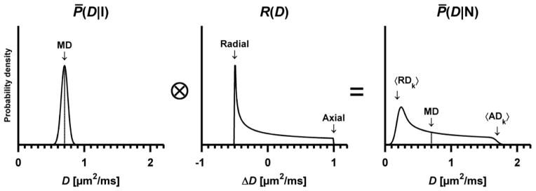
Schematic example of the distribution of diffusion coefficients when employing encoding that is isotropic (left, P̄(D|I)) and anisotropic (right, P̄(D|N)). The convolution visualizes how the variance of P̄(D|I) is added to the variance of the anisotropy response function R(D), rendering the total variance in P̄(D|N). This example depicts a system that contains axially symmetric and randomly oriented domains where MD_k = 0.70 ± 0.05 μm²/ms, and the axial and radial domain diffusion is AD_k = MD_k + 1.0 μm²/ms and RD_k = MD_k − 0.5 μm²/ms, respectively (middle panel). Thus, the variance of the anisotropy response function is equal for all domains. The fact that the system contains anisotropic domains is reflected in the width of R(D), indicating that there is a difference between the eigenvalues of the domain tensors. The prolate symmetry of the domain tensors can be discerned from the shape of R(D), where the slow diffusion (RD_k) is the most probable while the fast diffusion (AD_k) is the least probable (Eriksson et al., 2013). Note that the area under each distribution equals unity, and that the y-axes have been adjusted to improve legibility.

3. Methods

3.1. Imaging protocols

Data was acquired using a Philips Achieva 3T system, equipped with 80 mT/m gradients with a maximum slew rate of 100 mT/m/ms on axis, and an eight channel head coil.

The in vivo experiment was designed to evaluate the validity of the μFA model and was therefore acquired using a high b-value sampling rate, employing ten equidistant b-values between 100 and 2800 s/mm². Thereby, the sequence was limited to five image slices. Each set of data (one set per subject) contained images prepared with both the isotropic qMAS and harmonically modulated anisotropic encoding (Figure 3). Harmonic modulation is preferred to trapezoidal encoding to ensure equal diffusion times for both types of encoding (Eriksson et al., 2013). All DW data were acquired using an echo time of 160 ms, repetition time of 2000 ms, 96×96 acquisition matrix, spatial resolution of 3×3×3 mm³, partial Fourier factor of 0.8, and a SENSE factor of 2. Regardless of encoding technique, each encoding block, before and after the 180°-pulse, lasted 62.5 ms. Anisotropic encoding was performed in 15 directions for each b-value using harmonically modulated gradients according to Lasič et al. (2014). The directions were distributed using an electrostatic repulsion scheme (Jones et al., 1999). The isotropic encoding was repeated 15 times per b-value. This resulted in equal amounts of images and scan time for both techniques. The combined scan time for the isotropic and anisotropic encoding sequences was 10:12 min.

Figure 3.

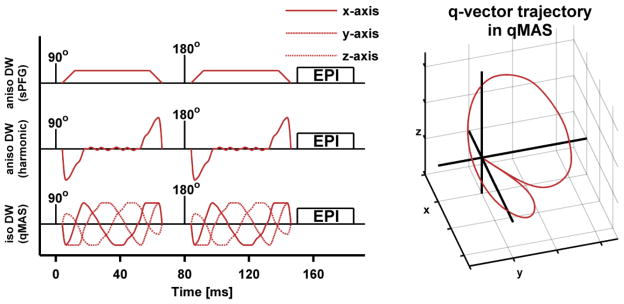
Schematic comparison of sequences (left) and qMAS q-vector trajectory (right). The sequences show a spin-echo experiment where different types of diffusion encoding blocks (red lines) have been inserted on both sides of the 180°-pulse. The first two rows show examples of anisotropic diffusion encoding that use trapezoidal and harmonic gradient modulation, respectively. The bottom row shows the harmonic gradient modulation in isotropic qMAS. The q-vector trajectory in the qMAS experiment (right) follows the surface of a cone with an aperture of twice the magic angle resulting in the same encoding strength in all directions for each encoding block. Note that the speed of the qMAS q-vector along the trajectory varies as a function of its magnitude (low magnitude entails low speed), and that the magnitude of the qMAS encoding is zero during the 180°-pulse.

Additionally, two whole-brain morphological sequences were acquired. One T1-weighted (T1W) 3D turbo-field-echo, reconstructed at a spatial resolution of 1×1×1 mm³; and one T2-weighted (T2W) FLAIR, reconstructed at a spatial resolution of 0.5×0.5×6 mm³. The scan time for the T1W and T2W images was 6:28 and 4:48 min, respectively.

3.2. Post-processing and parameterization

Motion correction and eddy-current correction was applied to DWI data using ElastiX (Klein et al., 2010). The first moment, and the second central moment of the distribution of diffusion coefficients was estimated by regressing the inverse Laplace transform of the gamma distribution function onto the acquired signal (Lasič et al., 2014; Roding et al., 2012). The signal was modeled, according to

$$\overline{S}(b)=S_0{\left(1+\frac{b·V}{\text{MD}}\right)}^{-\frac{{\text{MD}}^2}{V}},$$ Eq. 9

where MD and V were the fitting variables representing the initial slope and curvature of the signal attenuation function, respectively. Note that V in Eq. 9 corresponds to V_t and V_i when the model is regressed onto data from the powder averaged anisotropic and isotropic diffusion encoding experiments, respectively. Three constraints were introduced in the fitting procedure to eliminate non-physical results. First, the MD was constrained to be equal in the two acquisitions by assuming that 〈P̄(D|N)〉= 〈P̄(D|I)〉 = MD. This assumption is reasonable since the choice of encoding technique should not affect the mean diffusivity unless the diffusion time and the time required for the diffusing medium to probe the relevant restrictions are at the same scale, which is rarely the case for DWI in vivo (Nilsson et al., 2009; Nilsson et al., 2013). Second, V_i was constrained to the range between the total variance and zero (V_t ≥ V_i ≥ 0). Finally, signal that was attenuated below 5% (S̄(b) < 0.05 · S₀) was excluded from the fitting procedure. This was done to avoid detection of false variance in regions where a strong diffusion weighting rendered a signal that was elevated due to the noise floor. This is expected to affect only voxels where MD > 1.1 μm²/ms.

FA was calculated through conventional DTI analysis from the data employing anisotropic encoding for encoding strengths b ≤ 1000 s/mm². The μFA was calculated according to Eq. 8. Finally, the orientation coherence of the domains was quantified by the order parameter which is a well-established parameter for describing the order in liquid crystals. It is defined as OP = 〈(3 cos²(θ_k) − 1)/2〉, where θ_k is the angle between the domain and voxel scale symmetry axes. Thus, the OP provides a measure of orientation dispersion that has a simple geometric interpretation where OP = 1 indicates perfectly coherent alignment and OP = 0 indicates randomly oriented domain orientations. The OP can also be calculated from the microscopic and voxel scale variance, according to (Lasič et al., 2014)

$$\text{OP}=\sqrt{\frac{V_{\mathrm{\lambda }}}{\langle V_{\mathrm{\lambda },k}\rangle }}.$$ Eq. 10

Note that OP is not equivalent to the orientation dispersion index used in NODDI (Zhang et al., 2012), and that it can be calculated for any given orientation distribution function.

3.3. In vivo experiments

Imaging was performed on eight healthy volunteers (age 32 ± 4 years, all male) and two patients with brain tumors (one female, 62 years, with meningioma, WHO grade I; and one male, 46 years, with glioblastoma, WHO grade IV). Written consent was obtained from all subjects and the study was approved by the Regional Ethical Review Board at Lund University.

Analysis of diffusion parameters was performed at the group level, as well as in a single representative subject. Three regions of interest (ROI) were selected in the WM; the splenium of the corpus callosum (CC), the corticospinal tract (CST), and the anterior crossing region (CR) where frontal projection fibers from the genu of the corpus callosum and thalamic radiation of the internal capsule intersect (see Assaf and Pasternak (2008)). One ROI was also placed in the superior part of the thalamus (THA), which contains a mixture of WM and GM. The ROIs were delineated manually, using MD, FA and μFA maps for guidance; the operator was instructed to avoid voxels that contained GM or CSF.

The healthy individual was investigated with respect to the signal parameterization and parameter distribution in all four ROIs. One additional ROI was placed in the lateral ventricles to investigate the signal attenuation in the isotropic and rapidly diffusing CSF. The analysis of the parameter distribution was based on the ROIs while the signal and model fit was inspected in a single voxel in each ROI. Further, the voxel-wise correlation between combinations of FA, μFA and OP were evaluated. This analysis was performed in one axial slice of the image volume and the parameter maps were masked to remove interference from irrelevant regions of the head. The strength of the association was quantified by the coefficient of determination (r², Pearson’s linear correlation coefficient squared).

The healthy volunteer group was investigated with respect to the parameter distribution in the CC, CST, CR and THA. In order to elucidate if the three WM regions were different with respect to parameter mean values, F-tests (one-way ANOVA, assuming independent samples) were performed on the distributions of MD, FA, μFA, OP, V_i and V_a in the CC, CST and CR. The threshold for significance was set at α = 0.05/6 (Bonferroni correction for six tests).

The tumors were compared with respect to their FA and μFA by placing ROIs in one axial slice through each tumor. The ROIs were defined manually and the inclusion of WM, GM and CSF was avoided. Both tumors were resected one day after the MRI procedure and histological evaluation of the tumors was performed, in accordance with local clinical routine. Each tumor specimen was fixed in 4% buffered formaldehyde solution, embedded in paraffin, and sectioned at 4 μm. The sections were stained with hematoxylin-eosin in order to visualize the tissue structure and cell morphology. Microscopy was performed on an Olympus BX50. The cell shape and presence of tissue fascicles was investigated qualitatively and compared to corresponding diffusion parameters. Finally, structure tensor analysis (Peyré, 2011) was performed on the microphotos to enhance the visibility of cell structure orientations.

3.4. Simulation experiments

Simulation experiments were performed to investigate the qualitative behavior of FA and μFA in scenarios where the underlying system contained complex diffusion profiles. These scenarios were designed to mimic a range of effects that may be found in experimental data. The results were evaluated in terms of the value, effect size, effect direction, and accuracy of the FA and μFA.

The simulations included three types of model components (C) with varying water fractions (f). The first component was designed to represent the anisotropic diffusion in WM (C_a). For simplicity, all anisotropic domains were assumed to be axially symmetric and were described by their radial (RD_k) and axial diffusivity (AD_k). These were set to AD_k = 1.7 and RD_k = 0.2 μm²/ms. The orientation dispersion was modeled with the Watson distribution (Sra and Karp, 2013; Zhang et al., 2011) where the concentration parameter (κ) is related to the order parameter according to

$$\text{OP}=\frac{1}{2}·\frac{\mathcal{M}(3/2,5/2,\kappa )}{\mathcal{M}(1/2,3/2,\kappa )-1},$$ Eq. 11

where is the confluent hypergeometric function. The order parameter could be varied to produce geometries between fully coherent (OP = 1) and fully dispersed (OP = 0) orientations. The two remaining environments were designed to represent diffusion in damaged neural tissue (C_i) and CSF (C_CSF). The diffusion in these environments was assumed to be isotropic, with a domain mean diffusivity of MD_k = 1.7 and 3.0 μm²/ms in C_i and C_CSF, respectively.

Damaged WM was simulated by gradually replacing C_a with C_i. This was done in four geometries; the first three included one, two and three coherent (OP = 1) and orthogonal C_a components, and the last contained one C_a component with randomly oriented domains (OP = 0). The isotropic component replaced one anisotropic component while the remaining anisotropic components were unaltered. For example, in the case of two crossing fibers (C_a1 and C_a2), the damaged anisotropic component C_a1, had a volume fraction f_a1. Initially, f_a1 made up half the volume, but was gradually reduced to zero, and the fraction lost in C_a1 was replaced by C_i, i.e., f_a1 = 1/2 → 0, and f_i = 1/2 − f_a1. During this process the fraction of C_a2 was constant (f_a2 = 1/2).

The response to increasing radial diffusivity, mimicking demyelination, was simulated in a coherent C_a component (OP = 1), where the radial diffusivity was increased from its starting value until it exhibited no anisotropy (RD_k = 0.2 → 1.7 μm²/ms). Effects of orientation dispersion were investigated using a single C_a component with variable amount of dispersion, from dispersed to coherent (OP = 0 → 1). The effect of the crossing angle between two coherent C_a components was simulated by varying the angle from a parallel to a perpendicular geometry (φ = 0 → 90°). Finally, the effects of CSF contamination were simulated by gradually replacing a coherent C_a component (OP = 1) with C_CSF (f_a = 1 → 0, and f_CSF = 1 − f_a). In all cases, the effects of noise were simulated for five equidistant points along each process by adding Rice-distributed noise to the signal (Sijbers and den Dekker, 2004). The signal was generated in accordance with the imaging protocol, i.e., using the same b-values, number of directions and parameterization, at a S₀ signal-to-noise ratio (SNR) of 20. The model was regressed onto 1000 realizations of the noisy signal to render a reliable median and inter quartile range of the parameters.

4. Results

4.1. In vivo experiments

Maps of FA, μFA and OP for one healthy volunteer are shown in Figure 4. As expected, the μFA is high in regions comprised of WM and lower in GM. Most notably, the FA and μFA maps differ in regions where a high orientation dispersion is expected, for example, in crossing WM and the interface between WM pathways, in accordance with Lawrenz and Finsterbusch (2014). Another prominent difference can be seen in the GM where FA is close to zero, whereas μFA indicates that the GM contains detectable microscopic anisotropy. Figure 5 shows the parameter distribution in the CC, CST, CR, THA and CSF, and the powder averaged signal originating from a single voxel in each region. As expected for WM tissue, the departure from monoexponential attenuation was smaller for the isotropic encoding than the anisotropic encoding. The THA exhibited a relatively high isotropic variance, but the presence of microscopic anisotropy is clearly visible from the separation of the two signal curves. In the CSF, the signal was attenuated below 5% of its initial value, and it is apparent that the fitting would detect a false variance if high b-value data was not excluded. The resulting parameterization of the signal seen in Figure 5 was: μFA = 0.98, 1.03, 0.96, 0.76, 0.00; MD = 0.91, 0.84, 0.89, 1.60, 2.95 μm²/m; V_i = 0.07, 0.00, 0.01, 1.66, 0.01 μm⁴/ms²; and V_a = 0.57, 0.66, 0.51, 0.65, 0.00 μm⁴/ms² in the CC, CST, CR, THA and CSF, respectively.

Figure 4.

T1W, μFA, FA and OP maps from one healthy volunteer. The μFA is similar to the FA map in that it highlights the WM of the brain, but does so regardless of the local orientation dispersion. The μFA exhibits high values in areas where FA values are low due to crossing, bending and fanning fibers. Thus, the μFA map exhibits strong resemblance to the WM morphology in the T1W image, although the latter is not quantitative. The GM is visible in the μFA-map at a slightly lower intensity, indicating that the microscopic anisotropy is lower in GM as compared to WM. The OP displays similar contrast to the FA, in regions of WM.

Figure 5.

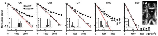
Signal vs. b curves and parameter distributions in the corpus callosum (CC), corticospinal tract (CST), anterior crossing region (CR), thalamus (THA) and the cerebrospinal fluid in the lateral ventricles (CSF) in one healthy volunteer. The ROIs are shown in the FA map (right, black-white outline). The signal plots show the powder averaged signal from a single voxel in each region as measured with isotropic and anisotropic diffusion encoding (white and black circles), as well as the model fit (dashed and solid lines). The red lines are a visual reference showing monoexponential attenuation at the estimated mean diffusivity. The signal attenuation in all three WM regions is similar, where the isotropic encoding shows little deviation from monoexponential attenuation, while the anisotropic encoding exhibits a curvature in the signal attenuation, indicating that all regions contain microscopic anisotropy. In the THA, both the isotropic and anisotropic encoding shows a strong deviation from monoexponential attenuation, although the presence of microscopic anisotropy is made clear by the separation of the two curves. Note that the signal from the CSF was fitted only for signal values above 5% of the signal at b = 0 s/mm², and that the y-axis in the CSF plot has a larger range than the other plots. The inserted histograms show the parameter distribution in each ROI where black and white bars represent FA and μFA, respectively. The histograms show that the μFA is similar in the three WM ROIs and that the largest difference between FA and μFA can be found in the CR and THA.

The voxel-wise correlation between μFA, OP and FA is presented in Figure 6. The relation between FA and μFA resembles the relation between the corresponding parameters reported by Jespersen et al. (2013) in that high FA entails high μFA, although not vice versa. The correlation between μFA and FA was found to exhibit two distinct modes, which were separated by introducing an arbitrary threshold at the shoulder of the distribution (μFA = 0.8). The interval containing high values of μFA was found to correspond well to regions of WM (μFA > 0.8, red outline in Figure 6) and the low μFA was found in a mixture of peripheral WM, GM and CSF (μFA < 0.8, white outline in Figure 6). In the WM region, a strong correlation was found between OP and FA (r² = 0.9), while only weak correlations were found between μFA and OP (r² = 0.1), and between μFA and FA (r² = 0.4). No relevant correlations were found in the peripheral region (all r² < 0.3).

Figure 6.

Voxel-wise parameter dependency between FA, μFA and OP in one healthy volunteer. The strongest correlation was found for the OP and FA (top left, see text for details). Separating the distribution at a threshold of μFA = 0.8 (red and black dots show μFA above and below 0.8, respectively) revealed a clear spatial dependency where high values of μFA are associated with the WM of the brain (voxels within red outline). The correlation between OP and FA in the WM indicates that FA is strongly dependent on the OP, i.e., the FA is strongly dependent on the coherence of WM fibers.

The investigation of the parameter distribution in the group of healthy volunteers is summarized in Table 1. All parameter mean values, except the MD and V_i, were found to have significantly different mean values in the three WM ROIs. This was expected for the FA since the ROIs include both coherent and crossing WM tissue. The μFA was also found to differ significantly between the three regions, albeit at a much smaller effect size compared to the FA. The group level variability detected in MD and V_i indicated that the absence of significance is likely due to a small effect size and large variance, respectively.

Table 1.

Diffusion parameters (group mean ± standard deviation) in four ROIs in the group of healthy volunteers (n = 8). The ANOVA indicated significantly different mean values in the CC, CST and CR for all parameters except MD and V_i. Note that the number of voxels in each ROI (#Vox) is shown but was not included in any tests.

	THA	CC	CST	CR
MD [μm2/ms]	1.09 ± 0.20	0.98 ± 0.11	0.96 ± 0.05	1.00 ± 0.06
FA	0.31 ± 0.04	0.86 ± 0.03	0.64 ± 0.04	0.38 ± 0.04†
μFA	0.82 ± 0.09	1.02 ± 0.02	0.97 ± 0.01	0.93 ± 0.01†
OP	0.26 ± 0.02	0.64 ± 0.04	0.47 ± 0.03	0.27 ± 0.03†
Va [μm4/ms2]	0.50 ± 0.12	0.96 ± 0.19	0.65 ± 0.07	0.57 ± 0.07†
Vi [μm4/ms2]	0.54 ± 0.40	0.30 ± 0.21	0.17 ± 0.05	0.22 ± 0.11
#Vox	12 ± 3	5 ± 3	32 ± 5	24 ± 5

^†ANOVA shows significant difference between parameter mean values (p ≪ 0.05/6) in the CC, CST and CR.

The anisotropy parameters measured in the two tumor types are presented in Figure 7, and corresponding microphotos of the excised tumors are presented in Figure 8. The meningioma tissue exhibited a low voxel scale anisotropy (mean ± standard deviation, FA = 0.19 ± 0.06) and high microscopic anisotropy (μFA = 0.88 ± 0.08). Likewise, the glioblastoma tissue exhibited low voxel scale anisotropy (FA = 0.07 ± 0.05). However, it exhibited markedly lower microscopic anisotropy compared to the meningioma (μFA = 0.39 ± 0.22). Although both tumors exhibited low FA values, the FA in the meningioma was elevated compared to the glioblastoma, indicating that the tissue is organized enough to create a weak but detectable diffusion anisotropy on the voxel scale. The high vs. low microscopic anisotropy in the meningioma and glioblastoma was corroborated by the histological examination of the two tumors, shown in Figure 8. The histological examination of the meningioma demonstrated a dense fascicular pattern of growth with elongated tumor cells, consistent with low FA and high μFA; and a more loose assemblage of rounded cells of variable size along with patchy areas of necrosis in the glioma, consistent with both low FA and low μFA.

Figure 7.

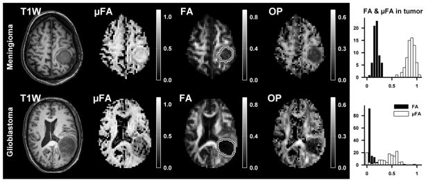
Parameter maps from the meningioma (top row) and glioblastoma (bottom row). The ROIs used for quantitative evaluation of diffusion parameters are shown in the FA maps (white-black outline). Both tumors exhibited low FA, while the μFA was high in the meningioma and low in the glioblastoma (histogram).

Figure 8.

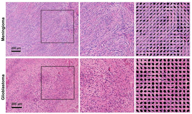
Microphotos of excised meningioma (top row) and glioblastoma (bottom row) tissue. The meningioma exhibited a dense fascicular pattern of growth with elongated tumor cells in a mostly monomorph structure. As seen in the upper left image, the fascicles in the meningioma could stretch for distances comparable to the voxel size (~1 mm). The glioblastoma exhibited a loose assemblage of rounded cells of variable size, along with patchy areas of necrosis. Blood vessels had thickened walls with endothelial cell proliferation and multiple small bleedings were included. The images on the right show magnified areas of the tumor tissue as well as structure tensors (black ellipses) that illustrate the local orientation of the tissue. The structure tensors in the meningioma showcase the presence of locally ordered structures, while few such structures are appear in the glioblastoma.

4.2. Simulation experiment

Figure 9 and Figure 10 showcase how the FA and μFA are altered when the underlying diffusion profiles are manipulated.

Figure 9.

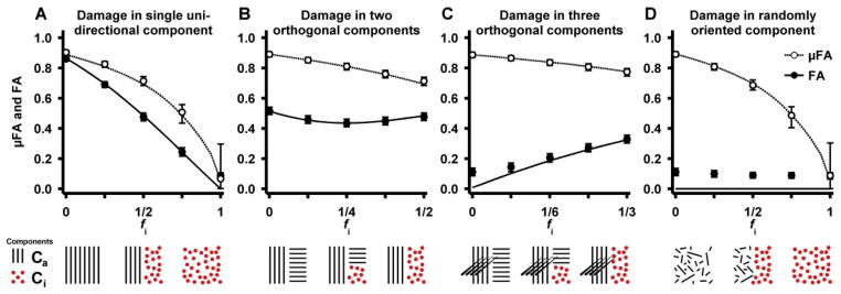
Response in FA and μFA in four geometries where one anisotropic component is replaced by an isotropic component to mimic tissue damage. The solid and broken lines show the noise free FA and μFA, respectively. The circular markers show the median parameter value when the SNR is 20, using the imaging protocol and parameterization detailed in the methods section. The error bars show the influence of noise as the inter quartile range. The geometries and processes are illustrated with graphics below the plots showing the anisotropic (black lines) and isotropic components (circles). Generally, the FA and μFA differ in all processes. In the single damaged WM component (A), the FA and μFA should be equal, but a positive bias in the μFA is induced due to the increasing presence of the isotropic component. In the double crossing (B), the FA can both increase and decrease due to the selective removal of anisotropic domains, whereas the μFA is strictly decreasing as a function of the reduction of anisotropy. In the triple crossing (C), the FA and μFA exhibit opposing effects, where FA increases and μFA decreases. The randomly oriented domains (D) illustrate that FA has no sensitivity to any changes in this case, while the μFA still reflects the presence of microscopic anisotropy.

Figure 10.

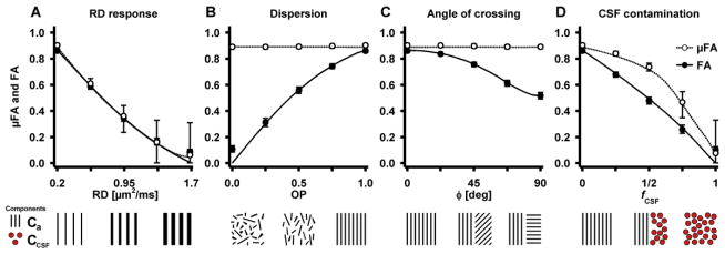
Response in FA and μFA due to changes in microstructure geometry. The plot objects are described in the caption of Figure 9. The response to increasing radial diffusivity (A) is equivalent for FA and μFA, however, the quantification of μFA displays a higher uncertainty. Both the effects of dispersion (B) and angle of crossing (C) have no effect on the μFA, while the FA is strongly modulated. The effect of CSF contamination (D) shows a positive bias in μFA compared to FA, similar to that found in Figure 9A. Note that the values of FA and μFA in the simulation of CSF contamination are expected to be lower than the corresponding values in Figure 9A. The similarity arises from the model fitting, where the bias is positive in both cases, but more so in the case of CSF since the model violation is larger. The varying degree of bias works to counteract the underlying difference between the two environments. Generally, in environments with low levels of microscopic anisotropy, μFA exhibits a higher level of statistical uncertainty as compared to FA. Note that the noise prevents both FA and μFA from assuming values close to zero.

When a coherent anisotropic component was replaced by an isotropic component (Figure 9A), the FA decreased approximately linearly as a function of the isotropic tissue fraction. In the same system, the μFA followed a similar pattern, but had a less pronounced initial slope indicating that the μFA is overestimated when the distribution of diffusion coefficients contains both isotropic and anisotropic components. In the absence of noise, both parameters approached zero for purely isotropic systems. In the crossing geometry, where one anisotropic component was replaced by an isotropic component (Figure 9B), the FA first decreased due to the relatively rapid increase of the isotropic component. However, when a majority of the receding component had been removed (f_i > 1/2), the FA instead increased due to the dominance of the remaining anisotropic component. By contrast, μFA decreased strictly. This demonstrates a case where μFA may exhibit superior sensitivity and specificity over FA, since the direction of the effect is constant. Further, the effect size is larger for μFA since it is not confounded by the same counteracting mechanisms. Similar results are shown for a triple crossing geometry (Figure 9C). In this case the FA started at a low value because the tissue was macroscopically isotropic with its three orthogonal fiber populations, and increased as one of the fiber populations was replaced by isotropic tissue. Again, the positive direction of the effect, caused by the reduction in orientation dispersion, may be confounding. By contrast, μFA reflected only the presence of microscopic anisotropy and responded as expected to the simulated damage. In the case of damage in randomly oriented micro domains (Figure 9D), the macroscopic anisotropy is zero, rendering FA insensitive to any changes in tissue microstructure while the μFA reflects the amount of microscopic anisotropy that is lost.

The effect of gradually increasing domain radial diffusivity, resulted in similar effects for FA and μFA (Figure 10A). However, as the system approaches isotropic conditions, the uncertainty in the μFA increases considerably. Figure 10B shows how dispersion influences the FA, while the μFA is constant. A similar pattern is seen when simulating crossing fibers with varying crossing angles (Figure 10C). As expected the FA was highest when the two fiber structures were parallel and had its lowest value when they were perpendicular. These results show the potential benefits of quantifying a measure for anisotropy that is not sensitive to confounds such as crossing, bending, fanning, and kissing fiber geometries. Finally, the effects of CSF contamination exhibit similar effects as the simulated damage in a single coherent WM system (compare Figure 9A and Figure 10D). This simulation highlights the overestimation of μFA due to multiple isotropic components. Generally, the μFA is increasingly susceptible to noise as the simulated systems approach zero microscopic anisotropy, resulting in reduced accuracy.

5. Discussion

In this study we present the first implementation of qMAS for the purpose of probing the microscopic anisotropy in vivo on a clinical MRI system. The parameters μFA and OP, as well as conventional DTI parameters FA and MD, were quantified in healthy subjects and in two different types of tumor tissue. Unlike the voxel scale anisotropy, measured in terms of the FA, the microscopic anisotropy measured by μFA was relatively homogeneous in large portions of the WM. This finding is in agreement with other studies that have aimed to remove effects of orientation dispersion from the quantification of local anisotropy (Jensen et al., 2014; Jespersen et al., 2013; Lawrenz and Finsterbusch, 2013, 2014). The notion that FA is sensitive to local orientation dispersion is supported by the strong correlation found between the FA and OP (Figure 6). However, the three WM regions chosen for analysis exhibited small but statistically significant differences also in μFA (Table 1), indicating that orientation dispersion is not the only difference between these regions. This could possibly be explained by varying levels of domain anisotropy, for example, caused by variable axonal packing density.

In the tumor tissue, FA was generally low, which indicated that the meningioma and the glioblastoma were approximately isotropic on the voxel scale. By contrast, the μFA was able to reliably differentiate between the two tumors, and indicated that microscopic diffusion anisotropy was more pronounced in the meningioma than the glioblastoma. Thus, the information provided by both FA and μFA was instrumental in predicting the tumor cell structures which were later confirmed by the histological exam (Figure 8).

To elucidate some of the underlying mechanisms that affect FA and μFA, simulations of different micro-environments visualized the parameters as a function of several relevant processes. For example, in the case of increased radial diffusivity of parallel fibers, the responses in FA and μFA are approximately equal, meaning that the two representations of anisotropy share a common interpretation. On the other hand, scenarios that include any form of orientation dispersion demonstrate prominent differences between FA and μFA. For example, the combination of two and three orthogonal anisotropic components (Figure 9B and C) were used to reproduce the effects of selective atrophy in a crossing WM geometry, as reported by Douaud et al. (2011), where the effect direction in FA was found to be positive in a damaged region of crossing WM. The simulations also illuminated the bias that arises when μFA is quantified in systems that violate the assumptions used in the parameterization, e.g., in complex mixtures of anisotropic and isotropic tissue. Although these scenarios invalidate the μFA as a direct metric of the microscopic anisotropy, it is worth noting that it retains sensitivity to the relevant effect and does so in a more consistent manner than the FA.

Although the comparison between FA and μFA showcases the effects of orientation dispersion as a confounder for FA, it does not invalidate previous studies that employ FA as a biomarker. Instead, the origin of the effect can be better understood, possibly allowing an improved interpretation of the FA and its relation to the microstructural integrity. We expect that μFA may not only contribute to the investigation of complex WM geometries, but also in detecting microscopic anisotropy in tissues that are approximately isotropic on the voxel scale, for example, in GM (McNab et al., 2013; Truong et al., 2014). Further, the μFA and OP may provide complementing information to the FA and tensor shape analysis previously used in the differentiation of classic and atypical meningioma (Toh et al., 2008), detection of fibroblastic meningioma (Tropine et al., 2007), and in the preoperative estimation of tumor consistency (Kashimura et al., 2007), by removing the confounding effects of orientation dispersion which are otherwise ignored.

It is important to stress that the signal acquired with conventional anisotropic encoding used in this study is identical to that needed for DKI analysis. However, because DKI makes no effort to distinguish between the origins of the diffusional kurtosis (herein referred to as variance in diffusion coefficients) it is not directly associated to microscopic anisotropy. The framework presented here is also related to the dPFG-methods employed by Jespersen et al. (2013) and Lawrenz and Finsterbusch (2014). In terms of the analysis presented here, dPFG encoding can be described with an encoding tensor which renders a signal that is sensitive to a weighted sum of V_i and V_a, where the weighting depends on the direction of the encoding blocks (Westin et al., 2014). It appears that the framework based on qMAS combined with anisotropic encoding probes the μFA more directly and may therefore provide a faster technique for measuring microscopic anisotropy compared to the dPFG methods. Finally, we note that the implementation and use of qMAS is no more complicated than a similar DKI protocol. Other techniques that take orientation dispersion into account include, for example, NODDI which quantifies the magnitude of fiber dispersion and the neurite density (Zhang et al., 2012). From this information it is possible to calculate a parameter analogous to the μFA. However, like DTI and DKI, the NODDI technique cannot distinguish between randomly oriented anisotropic domains and multiple isotropic components. Another drawback of model-based approaches, such as NODDI, is the demand for a priori assumptions about the tissue that is investigated, which may limit their use in abnormal tissues such as tumors.

In the present study, several factors affected the accuracy, i.e., the trueness and precision, of the estimated μFA. The imaging protocol features a long echo time which impacted the SNR and thus also the precision of μFA. Sufficient SNR for a robust signal parameterization was achieved by increasing the voxel size. Consequently, this increased the amount of PVE, especially in tissue interfacing with CSF, thereby reducing the trueness in such regions. Note that the present protocol was designed to test the validity of the suggested model by acquiring a densely sampled signal. However, the experimental design can be adjusted to allow whole brain coverage at feasible acquisition times by optimizing the acquisition protocol (Alexander, 2008). Further, a relatively low number of encoding directions were acquired, which may have reduced the trueness by introducing a weak directional dependency in the powder averaged signal, although simulations (data not shown) indicate a negligible μFA bias even for highly anisotropic tissue. A further limitation of μFA is that it may suffer from low accuracy when the model assumptions are violated or when investigating tissue with little or no microscopic anisotropy. The effects of such unfavorable conditions are demonstrated in the simulations (Figure 9 and Figure 10). The reduced accuracy in tissue with low anisotropy (μFA < 0.4) can be understood by considering Eq. 7 for V_a approaching zero; where the restriction on V_a to be positive may reduce trueness, and low levels of variance in V_a will render a poor precision in μFA. Thus, it is likely that the μFA calculated in the glioblastoma exhibited a positive bias since the histological exam of the glioblastoma found few anisotropic structures (Figure 8). Although the accuracy of the estimated μFA in the glioblastoma may be poor, the tumors could be reliably differentiated based on the difference in their microscopic anisotropy. Finally, a limitation may be that the assumption of Gaussian diffusion is not valid, i.e., that the signal attenuation may be dependent on diffusion time. We do not expect this to be the case in white matter for the current diffusion time regime (Nilsson et al., 2009; Nilsson et al., 2013). However, tumor tissue may contain larger cell structures, which could make μFA dependent on experimental parameters. This is a topic that deserves further attention, especially since qMAS exhibits an anisotropic time dependency due to the varying speed of the q-vector through q-space (Figure 3).

6. Conclusion

This study demonstrates the feasibility of mapping the microscopic anisotropy of the brain in vivo in terms of the μFA. The results suggest that the contrast found in conventional FA maps is strongly modulated by the orientation dispersion of the anisotropic domains contained within each imaging voxel. By contrast, our analysis quantifies the microscopic anisotropy and orientation dispersion separately in terms of the μFA and OP. Unlike the conventional FA derived from DTI, μFA may therefore provide a robust biomarker that probes the relevant diffusion anisotropy even in complex WM configurations. The potential benefit of μFA was demonstrated in two brain tumors. Although both tumors appeared isotropic on the voxel scale, the μFA could be used to distinguish between them based on their microscopic anisotropy. Additionally, simulations of complex tissue microstructures suggested that μFA exhibits a more intuitive interpretation than FA.

We predict that the combination of FA, μFA and OP can be useful in clinical and research applications, by enabling detection of microstructural degeneration in complex neural tissue, detection of fibrous tissue in tumors for pre-surgical classification of consistency, and quantification of microscopic anisotropy in macroscopically isotropic tissue.

Article Highlights.

• Microscopic anisotropy and orientation dispersion measured separately as μFA and OP

• First in vivo demonstration of μFA and OP imaging in volunteers and patients

• Isotropic diffusion encoding based on magic angle spinning of the q-vector

• In white matter, μFA is more specific to diffusion anisotropy than FA

• μFA correctly predicted cell shapes in meningioma and glioblastoma tumors

References

- Alexander AL, Hasan KM, Lazar M, Tsuruda JS, Parker DL. Analysis of partial volume effects in diffusion-tensor MRI. Magn Reson Med. 2001;45:770–780. doi: 10.1002/mrm.1105. [DOI] [PubMed] [Google Scholar]
- Alexander DC. A general framework for experiment design in diffusion MRI and its application in measuring direct tissue-microstructure features. Magn Reson Med. 2008;60:439–448. doi: 10.1002/mrm.21646. [DOI] [PubMed] [Google Scholar]
- Assaf Y, Pasternak O. Diffusion tensor imaging (DTI)-based white matter mapping in brain research: A review. J Mol Neurosci. 2008;34:51–61. doi: 10.1007/s12031-007-0029-0. [DOI] [PubMed] [Google Scholar]
- Basser PJ, Mattiello J, Le Bihan D. MR diffusion tensor spectroscopy and imaging. Biophys J. 1994;66:259–267. doi: 10.1016/S0006-3495(94)80775-1. [DOI] [PMC free article] [PubMed] [Google Scholar]
- Basser PJ, Pierpaoli C. Microstructural and physiological features of tissues elucidated by quantitative-diffusion-tensor MRI. J Magn Reson. 1996:209–2019. doi: 10.1006/jmrb.1996.0086. [DOI] [PubMed] [Google Scholar]
- Butts K, Pauly J, de Crespigny A, Moseley M. Isotropic diffusion-weighted and spiral-navigated interleaved epi for routine imaging of acute stroke. Magn Reson Med. 1997;38:741–749. doi: 10.1002/mrm.1910380510. [DOI] [PubMed] [Google Scholar]
- De Santis S, Drakesmith M, Bells S, Assaf Y, Jones DK. Why diffusion tensor MRI does well only some of the time: Variance and covariance of white matter tissue microstructure attributes in the living human brain. Neuroimage. 2013;89C:35–44. doi: 10.1016/j.neuroimage.2013.12.003. [DOI] [PMC free article] [PubMed] [Google Scholar]
- Douaud G, Jbabdi S, Behrens TE, Menke RA, Gass A, Monsch AU, Rao A, Whitcher B, Kindlmann G, Matthews PM, Smith S. DTI measures in crossing-fibre areas: Increased diffusion anisotropy reveals early white matter alteration in mci and mild alzheimer’s disease. Neuroimage. 2011;55:880–890. doi: 10.1016/j.neuroimage.2010.12.008. [DOI] [PMC free article] [PubMed] [Google Scholar]
- Englund E, Sjobeck M, Brockstedt S, Latt J, Larsson EM. Diffusion tensor MRI post mortem demonstrated cerebral white matter pathology. J Neurol. 2004;251:350–352. doi: 10.1007/s00415-004-0318-2. [DOI] [PubMed] [Google Scholar]
- Eriksson S, Lasič S, Topgaard D. Isotropic diffusion weighting in PGSE nmr by magic-angle spinning of the q-vector. J Magn Reson. 2013;226:13–18. doi: 10.1016/j.jmr.2012.10.015. [DOI] [PubMed] [Google Scholar]
- Hsu JL, Van Hecke W, Bai CH, Lee CH, Tsai YF, Chiu HC, Jaw FS, Hsu CY, Leu JG, Chen WH, Leemans A. Microstructural white matter changes in normal aging: A diffusion tensor imaging study with higher-order polynomial regression models. Neuroimage. 2010;49:32–43. doi: 10.1016/j.neuroimage.2009.08.031. [DOI] [PubMed] [Google Scholar]
- Jensen JH, Helpern JA, Ramani A, Lu H, Kaczynski K. Diffusional kurtosis imaging: The quantification of non-gaussian water diffusion by means of magnetic resonance imaging. Magn Reson Med. 2005;53:1432–1440. doi: 10.1002/mrm.20508. [DOI] [PubMed] [Google Scholar]
- Jensen JH, Hui ES, Helpern JA. Double-pulsed diffusional kurtosis imaging. NMR Biomed. 2014;27:363–370. doi: 10.1002/nbm.3030. [DOI] [PubMed] [Google Scholar]
- Jespersen SN, Lundell H, Sønderby CK, Dyrby TB. Orientationally invariant metrics of apparent compartment eccentricity from double pulsed field gradient diffusion experiments. NMR Biomed. 2013;26:1647–1662. doi: 10.1002/nbm.2999. [DOI] [PubMed] [Google Scholar]
- Jespersen SN, Lundell H, Sønderby CK, Dyrby TB. Commentary on “microanisotropy imaging: Quantification of microscopic diffusion anisotropy and orientation of order parameter by diffusion MRI with magic-angle spinning of the q-vector”. Frontiers in Physics. 2014a;2:28. [Google Scholar]
- Jespersen SN, Lundell H, Sønderby CK, Dyrby TB. Erratum: Orientationally invariant metrics of apparent compartment eccentricity from double pulsed field gradient diffusion experiments. NMR Biomed. 2014b;27:738–738. doi: 10.1002/nbm.2999. [DOI] [PubMed] [Google Scholar]
- Jones DK, Horsfield MA, Simmons A. Optimal strategies for measuring diffusion in anisotropic systems by magnetic resonance imaging. Magn Reson Med. 1999;42:515–525. [PubMed] [Google Scholar]
- Kashimura H, Inoue T, Ogasawara K, Arai H, Otawara Y, Kanbara Y, Ogawa A. Prediction of meningioma consistency using fractional anisotropy value measured by magnetic resonance imaging. J Neurosurg. 2007;107:784–787. doi: 10.3171/JNS-07/10/0784. [DOI] [PubMed] [Google Scholar]
- Klein S, Staring M, Murphy K, Viergever MA, Pluim JP. Elastix: A toolbox for intensity-based medical image registration. IEEE Trans Med Imaging. 2010;29:196–205. doi: 10.1109/TMI.2009.2035616. [DOI] [PubMed] [Google Scholar]
- Kubicki M, Westin CF, Maier SE, Mamata H, Frumin M, Ersner-Hershfield H, Kikinis R, Jolesz FA, McCarley R, Shenton ME. Diffusion tensor imaging and its application to neuropsychiatric disorders. Harv Rev Psychiatry. 2002;10:324–336. doi: 10.1080/10673220216231. [DOI] [PMC free article] [PubMed] [Google Scholar]
- Lasič S, Szczepankiewicz F, Eriksson S, Nilsson M, Topgaard D. Microanisotropy imaging: Quantification of microscopic diffusion anisotropy and orientational order parameter by diffusion MRI with magic-angle spinning of the q-vector. Frontiers in Physics. 2014;2:11. [Google Scholar]
- Lawrenz M, Finsterbusch J. Double-wave-vector diffusion-weighted imaging reveals microscopic diffusion anisotropy in the living human brain. Magn Reson Med. 2013;69:1072–1082. doi: 10.1002/mrm.24347. [DOI] [PubMed] [Google Scholar]
- Lawrenz M, Finsterbusch J. Mapping measures of microscopic diffusion anisotropy in human brain white matter in vivo with double-wave-vector diffusion-weighted imaging. Magn Reson Med. 2014 doi: 10.1002/mrm.25140. [DOI] [PubMed] [Google Scholar]
- Lawrenz M, Koch MA, Finsterbusch J. A tensor model and measures of microscopic anisotropy for double-wave-vector diffusion-weighting experiments with long mixing times. J Magn Reson. 2010;202:43–56. doi: 10.1016/j.jmr.2009.09.015. [DOI] [PubMed] [Google Scholar]
- Lebel C, Walker L, Leemans A, Phillips L, Beaulieu C. Microstructural maturation of the human brain from childhood to adulthood. Neuroimage. 2008;40:1044–1055. doi: 10.1016/j.neuroimage.2007.12.053. [DOI] [PubMed] [Google Scholar]
- Löbel U, Sedlacik J, Gullmar D, Kaiser WA, Reichenbach JR, Mentzel HJ. Diffusion tensor imaging: The normal evolution of adc, ra, fa, and eigenvalues studied in multiple anatomical regions of the brain. Neuroradiology. 2009;51:253–263. doi: 10.1007/s00234-008-0488-1. [DOI] [PubMed] [Google Scholar]
- McNab JA, Polimeni JR, Wang R, Augustinack JC, Fujimoto K, Stevens A, Triantafyllou C, Janssens T, Farivar R, Folkerth RD, Vanduffel W, Wald LL. Surface based analysis of diffusion orientation for identifying architectonic domains in the in vivo human cortex. Neuroimage. 2013;69:87–100. doi: 10.1016/j.neuroimage.2012.11.065. [DOI] [PMC free article] [PubMed] [Google Scholar]
- Mitra P. Multiple wave-vector extensions of the nmr pulsed-field-gradient spin-echo diffusion measurement. Physical Review B. 1995;51:15074–15078. doi: 10.1103/physrevb.51.15074. [DOI] [PubMed] [Google Scholar]
- Nilsson M, Latt J, Stahlberg F, van Westen D, Hagslatt H. The importance of axonal undulation in diffusion MR measurements: A monte carlo simulation study. NMR Biomed. 2012;25:795–805. doi: 10.1002/nbm.1795. [DOI] [PubMed] [Google Scholar]
- Nilsson M, Lätt J, Nordh E, Wirestam R, Ståhlberg F, Brockstedt S. On the effects of a varied diffusion time in vivo: Is the diffusion in white matter restricted? Magn Reson Imaging. 2009;27:176–187. doi: 10.1016/j.mri.2008.06.003. [DOI] [PubMed] [Google Scholar]
- Nilsson M, van Westen D, Stahlberg F, Sundgren PC, Latt J. The role of tissue microstructure and water exchange in biophysical modelling of diffusion in white matter. MAGMA. 2013;26:345–370. doi: 10.1007/s10334-013-0371-x. [DOI] [PMC free article] [PubMed] [Google Scholar]
- Oouchi H, Yamada K, Sakai K, Kizu O, Kubota T, Ito H, Nishimura T. Diffusion anisotropy measurement of brain white matter is affected by voxel size: Underestimation occurs in areas with crossing fibers. AJNR Am J Neuroradiol. 2007;28:1102–1106. doi: 10.3174/ajnr.A0488. [DOI] [PMC free article] [PubMed] [Google Scholar]
- Peyré G. The numerical tours of signal processing - advanced computational signal and image processing. IEEE Computing in Science and Engineering. 2011;13:94–97. [Google Scholar]
- Roding M, Bernin D, Jonasson J, Sarkka A, Topgaard D, Rudemo M, Nyden M. The gamma distribution model for pulsed-field gradient nmr studies of molecular-weight distributions of polymers. J Magn Reson. 2012;222:105–111. doi: 10.1016/j.jmr.2012.07.005. [DOI] [PubMed] [Google Scholar]
- Rovaris M, Gass A, Bammer R, Hickman SJ, Ciccarelli O, Miller DH, Filippi CG. Diffusion MRI in multiple sclerosis. Neurology. 2005;65:1526–1532. doi: 10.1212/01.wnl.0000184471.83948.e0. [DOI] [PubMed] [Google Scholar]
- Santillo AF, Martensson J, Lindberg O, Nilsson M, Manzouri A, Landqvist Waldo M, van Westen D, Wahlund LO, Latt J, Nilsson C. Diffusion tensor tractography versus volumetric imaging in the diagnosis of behavioral variant frontotemporal dementia. PLoS One. 2013;8:e66932. doi: 10.1371/journal.pone.0066932. [DOI] [PMC free article] [PubMed] [Google Scholar]
- Scholz J, Klein MC, Behrens TE, Johansen-Berg H. Training induces changes in white-matter architecture. Nat Neurosci. 2009;12:1370–1371. doi: 10.1038/nn.2412. [DOI] [PMC free article] [PubMed] [Google Scholar]
- Shemesh N, Cohen Y. Microscopic and compartment shape anisotropies in gray and white matter revealed by angular bipolar double-pfg MR. Magn Reson Med. 2011;65:1216–1227. doi: 10.1002/mrm.22738. [DOI] [PubMed] [Google Scholar]
- Sijbers J, den Dekker AJ. Maximum likelihood estimation of signal amplitude and noise variance from MR data. Magn Reson Med. 2004;51:586–594. doi: 10.1002/mrm.10728. [DOI] [PubMed] [Google Scholar]
- Sjobeck M, Elfgren C, Larsson EM, Brockstedt S, Latt J, Englund E, Passant U. Alzheimer’s disease (ad) and executive dysfunction. A case-control study on the significance of frontal white matter changes detected by diffusion tensor imaging (DTI) Arch Gerontol Geriatr. 2010;50:260–266. doi: 10.1016/j.archger.2009.03.014. [DOI] [PubMed] [Google Scholar]
- Sra S, Karp D. The multivariate watson distribution: Maximum-likelihood estimation and other aspects. Journal of Multivariate Analysis. 2013;114:256–269. [Google Scholar]
- Stejskal EO, Tanner JE. Spin diffusion measurement: Spin echoes in the presence of a time-dependent field gradient. J Chem Phys. 1965;42:288–292. [Google Scholar]
- Sullivan EV, Pfefferbaum A. Diffusion tensor imaging and aging. Neurosci Biobehav Rev. 2006;30:749–761. doi: 10.1016/j.neubiorev.2006.06.002. [DOI] [PubMed] [Google Scholar]
- Surova Y, Szczepankiewicz F, Latt J, Nilsson M, Eriksson B, Leemans A, Hansson O, van Westen D, Nilsson C. Assessment of global and regional diffusion changes along white matter tracts in parkinsonian disorders by MR tractography. PLoS One. 2013;8:e66022. doi: 10.1371/journal.pone.0066022. [DOI] [PMC free article] [PubMed] [Google Scholar]
- Szczepankiewicz F, Latt J, Wirestam R, Leemans A, Sundgren P, van Westen D, Stahlberg F, Nilsson M. Variability in diffusion kurtosis imaging: Impact on study design, statistical power and interpretation. Neuroimage. 2013;76:145–154. doi: 10.1016/j.neuroimage.2013.02.078. [DOI] [PubMed] [Google Scholar]
- Teipel SJ, Grothe MJ, Filippi M, Fellgiebel A, Dyrba M, Frisoni GB, Meindl T, Bokde AL, Hampel H, Kloppel S, Hauenstein K. Fractional anisotropy changes in alzheimer’s disease depend on the underlying fiber tract architecture: A multiparametric DTI study using joint independent component analysis. J Alzheimers Dis. 2014;41:69–83. doi: 10.3233/JAD-131829. [DOI] [PubMed] [Google Scholar]
- Toh CH, Castillo M, Wong AM, Wei KC, Wong HF, Ng SH, Wan YL. Differentiation between classic and atypical meningiomas with use of diffusion tensor imaging. AJNR Am J Neuroradiol. 2008;29:1630–1635. doi: 10.3174/ajnr.A1170. [DOI] [PMC free article] [PubMed] [Google Scholar]
- Topgaard D. Isotropic diffusion weighting in PGSE nmr: Numerical optimization of the q-mas PGSE sequence. Microporous and Mesoporous Materials. 2013;178:60–63. [Google Scholar]
- Topgaard D, Lasič S. Patent: Analys för kvantifiering av mikroskopisk diffusionsanisotropi. 2013. (Analysis for the quantification of microscopic diffusion anisotropy). Language: Swedish. IPC: A61B5/055, G01N24/00, G01R33/563. Filed: 2012-05-04, Issued: 2013-11-05. [Google Scholar]
- Tropine A, Dellani PD, Glaser M, Bohl J, Ploner T, Vucurevic G, Perneczky A, Stoeter P. Differentiation of fibroblastic meningiomas from other benign subtypes using diffusion tensor imaging. J Magn Reson Imaging. 2007;25:703–708. doi: 10.1002/jmri.20887. [DOI] [PubMed] [Google Scholar]
- Truong TK, Guidon A, Song AW. Cortical depth dependence of the diffusion anisotropy in the human cortical gray matter in vivo. PLoS One. 2014;9:e91424. doi: 10.1371/journal.pone.0091424. [DOI] [PMC free article] [PubMed] [Google Scholar]
- Westin CF, Maier SE, Mamata H, Nabavi A, Jolesz FA, Kikinis R. Processing and visualization for diffusion tensor MRI. Medical Image Analysis. 2002;6:93–108. doi: 10.1016/s1361-8415(02)00053-1. [DOI] [PubMed] [Google Scholar]
- Westin CF, Szczepankiewicz F, Pasternak O, Özarslan E, Topgaard D, Knutsson H, Nilsson M. Measurement tensors in diffusion MRI: Generalizing the concept of diffusion encoding. Med Image Comput Comput Assist Interv. 2014;17 (Pt 5):217–225. doi: 10.1007/978-3-319-10443-0_27. [DOI] [PMC free article] [PubMed] [Google Scholar]
- Wong EC, Cox RW, Song AW. Optimized isotropic diffusion weighting. Magn Reson Med. 1995;34:139–143. doi: 10.1002/mrm.1910340202. [DOI] [PubMed] [Google Scholar]
- Vos SB, Jones DK, Jeurissen B, Viergever MA, Leemans A. The influence of complex white matter architecture on the mean diffusivity in diffusion tensor MRI of the human brain. Neuroimage. 2012;59:2208–2216. doi: 10.1016/j.neuroimage.2011.09.086. [DOI] [PMC free article] [PubMed] [Google Scholar]
- Vos SB, Jones DK, Viergever MA, Leemans A. Partial volume effect as a hidden covariate in DTI analyses. Neuroimage. 2011;55:1566–1576. doi: 10.1016/j.neuroimage.2011.01.048. [DOI] [PubMed] [Google Scholar]
- Zhang H, Hubbard PL, Parker GJ, Alexander DC. Axon diameter mapping in the presence of orientation dispersion with diffusion MRI. Neuroimage. 2011;56:1301–1315. doi: 10.1016/j.neuroimage.2011.01.084. [DOI] [PubMed] [Google Scholar]
- Zhang H, Schneider T, Wheeler-Kingshott CA, Alexander DC. Noddi: Practical in vivo neurite orientation dispersion and density imaging of the human brain. Neuroimage. 2012;61:1000–1016. doi: 10.1016/j.neuroimage.2012.03.072. [DOI] [PubMed] [Google Scholar]