

Abstract
Dilution factors are a critical component in estimating concentrations of so-called “down-the-drain” chemicals (e.g., pharmaceuticals) in rivers. The present study estimated the temporal and spatial variability of dilution factors around the world using geographically referenced data sets at 0.5° × 0.5° resolution. Domestic wastewater effluents were derived from national per capita domestic water use estimates and gridded population. Monthly and annual river flows were estimated by accumulating runoff estimates using topographically derived flow directions. National statistics, including the median and interquartile range, were generated to quantify dilution factors. Spatial variability of the dilution factor was found to be considerable; for example, there are 4 orders of magnitude in annual median dilution factor between Canada and Morocco. Temporal variability within a country can also be substantial; in India, there are up to 9 orders of magnitude between median monthly dilution factors. These national statistics provide a global picture of the temporal and spatial variability of dilution factors and, hence, of the potential exposure to down-the-drain chemicals. The present methodology has potential for a wide international community (including decision makers and pharmaceutical companies) to assess relative exposure to down-the-drain chemicals released by human pollution in rivers and, thus, target areas of potentially high risk. Environ Toxicol Chem 2014;33:447–452. © 2013 The Authors. Environmental Toxicology and Chemistry published by Wiley Periodicals, Inc. on behalf of SETAC. This is an open access article under the terms of the Creative Commons Attribution-NonCommercial-NoDerivs License, which permits use and distribution in any medium, provided the original work is properly cited, the use is non-commercial, and no modifications or adaptations are made.
Keywords: Down-the-drain chemicals, Modeling, Risk assessment, Catchment
INTRODUCTION
Over recent decades, scientists and regulators have had increasing concerns over the extent of the threat posed by chemicals discharged to water from domestic sources as opposed to industry or agriculture. Such chemicals include pharmaceuticals and personal care products, natural hormones (e.g., estrogens), and engineered nanoparticles (e.g., nanosilver, present in a variety of household products). Most of these substances enter freshwaters via wastewater disposal after consumer use; they are thus commonly referred to as “down-the-drain” chemicals. Scientists worldwide study the impact of the presence of such substances in freshwaters on the surrounding wildlife. For example, the magnitude of endocrine disruption in wild fish has been strongly related to steroid estrogen excretion from human population centers 1.
For most policy makers, regulators, and indeed the public, 2 important questions have arisen: What level of exposure is the aquatic wildlife subjected to, and what will be the impact in their country? The response of many countries to assess their particular situation, such as with endocrine disruption, has been to commission large-scale chemical and biological monitoring programs 1–3. These exercises are very expensive and time-consuming. The answer they provide may come many years after the issue was first raised, and the results may be ambiguous.
There are many modeling approaches that could be applied to estimate predicted environmental concentrations of down-the-drain chemicals in rivers 4. It was demonstrated that the temporal variability of down-the-drain chemical concentration in surface waters is driven mainly by the seasonal variability of river flows 5,6.
Some higher-tier models have been developed to better represent local geographic conditions and provide more accurate estimates of concentrations (e.g., Low Flows 2000 Water Quality eXtension model 7, QUAL2E 8, GREAT-ER 9). Unfortunately, such models are rarely applicable at national or continental scales as a result of a lack of data. Many countries do not have measured or modeled hydrological data, such as river flows; additionally, location and size of sewage treatment plants (STPs) are often unavailable. It was recently demonstrated that despite such a lack of local data, there is sufficient global-scale data and information to estimate global threats to human water security and river biodiversity 10.
Thus, the dilution factor—the ratio between the volume of freshwater available and the domestic sewage discharge—can be used as a surrogate to compare risk levels caused by chemical exposure between and within countries 11. We propose that a quantification of the national dilution factor for domestic effluent should be the first step in estimating the extent of the freshwaters that are at risk from domestically sourced chemicals. This factor would be relevant to assessing aquatic exposure to all down-the-drain chemicals.
In the present study, global grids of dilution factors at annual and monthly resolutions were generated using data sets of annual and monthly runoff and population. The present approach, similar to that of Vörösmaty et al. 10, builds on the method developed by Keller et al. 12 to estimate spatial variations of dilution factors at the global scale, using readily available 0.5° × 0.5° gridded data (≈55 km × 55 km at the equator) for the whole terrestrial land surface. The spatial and temporal variability of dilution factors within and between countries are then assessed using statistical measures such as the median. This approach was designed to assess 1) differences between and within countries in terms of dilution of down-the-drain chemicals, 2) monthly variations within a country, and 3) suitability of providing a unique national dilution factor for a country.
MATERIALS AND METHODS
Modeling approach
The present method was designed specifically to assess the environmental level of exposure to down-the-drain chemicals in surface waters across the globe, even in countries where data are scarce. For a country, a crude estimate of the predicted environmental concentration in raw wastewater (PECSEWAGE; mg/L) of a chemical can be derived from daily per capita consumption (U; mg/cap/d)
| (1) |
where W is the daily per capita domestic water use (L/cap/d). Assuming no in-stream degradation and no background concentration, the river predicted environmental concentration (PECRIVER) immediately after mixing can then be defined as
| (2) |
where DF is the dilution factor and F is the fraction of chemical removed during wastewater treatment, which can be either measured or extrapolated from laboratory tests.
The dilution factor is defined as follows
| (3) |
where Qr (m3/s) is the river flow at the outlet of the catchment and Qww (m3/s) is the total domestic wastewater effluent generated within the catchment. Using gridded data, the river flow can be calculated from globally distributed runoff estimates (R; mm/yr). For a catchment with the outlet in cell i, the river flow in cell  is
is
| (4) |
where A is the cell area (km2) and j is an index of all cells contributing to the catchment above cell i.
The total domestic wastewater effluent generated in a catchment is the total amount of water used for household purposes (e.g., food preparation, flushing toilets, bathing, and lawn watering) across the catchment. Using gridded data, for a catchment with the outlet in cell i,  (m3/s) is estimated by combining population estimates (P) and national per capita domestic water use (W; m3/cap/yr) estimates
| (5) |
For any grid cell i, the dilution factor (DFi) is then
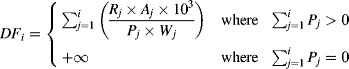 |
(6) |
The present approach assumes that all populations are connected to their nearby water courses, although sometimes a large proportion of a population may use septic tanks or a similar wastewater disposal in which the route to water is not direct. Such an assumption was made to provide a conservative estimate of the dilution factor; this estimate is likely to underestimate the dilution of chemicals discharged via humans and overestimate river predicted environmental concentration.
National summary statistics
The present approach may be applied at the catchment (within the limits of the grid size), national, or global scale using either annual or monthly runoff. Assessing the temporal and spatial variability in the dilution factor can address questions such as whether endocrine disruption in fish would be expected in only a few areas or be widespread across the nation. The median, mean, and a selection of percentiles—the interquartile ranges (25th and 75th percentiles), 5th, and 95th percentiles—were generated for each country; for each dilution factor map (annual and monthly), all cells within a country were identified and percentiles calculated across the selected grid cells. A percentile is the value of a variable below which a certain percentage of observations fall. The statistics within the present study were calculated using Microsoft Excel 2007.
While generating these statistics, the assumption was made that the dilution factor is only relevant where there is both river flow and wastewater effluent. Thus, for each country, these statistics were drawn only from cells where both the river flow and the total population in the upstream catchment were greater than 0. These statistics were calculated for both the annual and the monthly dilution factor grids.
Hydrological data
Runoff estimates can be derived using macro-scale hydrological models such as Macro-PDM 13, the variable infiltration capacity model 14, the water balance model 15, and Water-GAP2 16,17. A macro-scale model is a model that can be applied over a large geographic domain without calibration at the catchment scale 13. Such models were applied over recent years to estimate present and future water resource availability at global, continental, and regional scales 18–20.
In the present study, the annual and monthly composite runoff field data sets produced by Fekete et al. 21 at a spatial resolution of 0.5° × 0.5° were used. A climate-driven water mass balance was combined with observed river flow data to generate these long-term average runoff estimates. The water balance model uses climatologically averaged monthly air temperature and precipitation from an updated data set of Legates and Willmot climate fields 22,23. Runoff is then predicted based on soil type and texture from the Food and Agriculture Organization/United Nations Educational, Scientific and Cultural Organization soil data bank 24, topographic data from the global elevation data set ETOPO5 25, and a contemporary land-cover classification derived from overlaying cultivated areas from Olson's land-use classification 26 onto potential vegetation 27. The water balance model is then combined with observed river flow data from the Global Runoff Data Centre 28 using the global Simulated Topological Network at 30-minute spatial resolution (STN-30p) 29; the measured interstation runoff (difference between discharge downstream and discharge upstream), where available, was used to constrain the magnitude of the water balance modeled runoff. The time period of these river flow data varies for each gauging station; however, only those with at least 12 yr of records were selected. Approximately 60% of the gauging stations selected had the common data period 1970 to 1980. In the present study, the STN-30p was used to accumulate the annual and monthly runoff to estimate cell-specific river flow  .
.
Keller and Rees 30 assessed the goodness of fit of the flows derived from this approach using observed flow values from 670 gauging stations of the Global Runoff Data Centre. The measured flow data used in this assessment were not the same as the observed river flow data originally used by Fekete et al. 21 to estimate the composite runoff fields. The composite runoff fields method is most successful at simulating flows across Asia, North and Central America, Europe, and the Near East, with a mean bias between 0% and 10%. The method tends to overestimate observed flows across Africa and South America, with mean bias of 53% and 37%, respectively. For Australia and the Pacific, however, the method underestimates river flows (mean bias of –41%).
Population data
Population estimates are available from the SocioEconomic Data and Applications Centre. The Gridded Population of the World v.3 data set 31 is derived from population data issued by national bodies, such as national statistics offices, to generate gridded estimates of population, which are then adjusted to match United Nation totals. Here, the projected estimates for 2005 at 0.5° × 0.5° resolution were used; these 2005 estimates made use of census data up to 2004.
The dilution factors for each grid cell were calculated by applying Equation 6. It was therefore important that the population and runoff coverages matched adequately. An apparent mismatch occurs mostly along the coastlines, where the population coverage is wider in places, by 1 cell at the most, than the runoff coverage. The total population within the Gridded Population of the World v.3 data set is approximately equal to 6.4 × 10⁹ inhabitants; however, only 6.1 × 10⁹ inhabitants overlapped with the runoff coverage. The discrepency in population is approximately equal to 6% across the world, and similar discrepencies are observed at the national level (e.g., 3% for India and 5% for Egypt). Most statistics considered in the present study (median and 25th and 75th percentiles) are not sensitive to extreme values; thus, the impact of such a discrepency on the selected national dilution factor statistics was assumed to be negligible. However, the local dilution factor values along the coastlines must be handled with care as they might be underestimated (some of the coastal population discharge sewage effluent directly into the sea rather than into their local river; however, because of a lack of data, it was assumed that all coastal population discharges to rivers) or overestimated (as a consequence of the underestimated population [≈6%] when overlapping the runoff and the population coverage, the coastal population potentially discharging to rivers may be underestimated; this would result in underestimating the total domestic wastewater effluent and therefore overestimating the dilution factor [Equations 3 and 6]).
Domestic water use
In the present study, domestic water use was used as a proxy for wastewater discharge (Equation 1). There are significant variations in the amount of water used for domestic purposes between and within countries; these reflect differences in water availability as well as infrastructure, wealth, and habits. Although water-use data per country and per sector is among the most desired data in terms of water resources, the uncertainty within these data are often considerable. Furthermore, these data are often estimated rather than measured, with varying methods across data sources 32. These data should therefore also be handled with care.
Four main data sources for national per capita domestic water use were used to build a global data set: Gleick 32, Food and Agriculture Organization 33, World Resource Institute 34, and Organisation for Economic Co-operation and Development 35. Where discrepancies arose, only the data for the year 2000 or later were retained, and from these the lowest estimate was selected to provide a higher pollution scenario as it maximizes predicted environmental concentration in raw wastewater (Equation 1). The resulting set of mean values of national per capita domestic water use (W) was mapped at the country level, which was then disaggregated at a 0.5° × 0.5° resolution to produce gridded values of domestic water use across the globe (tabulated values in Supplemental Data, Table S1). It should be noted that the variability in stated per capita water consumption can be significant; for approximately 34% of countries with available data, there was at least a factor 2 between data sources, with 11 countries having more than a factor 5 between the lowest and the highest values.
At present, because of a lack of data, a single national average domestic water-use figure was used. However, in some countries, differences in domestic water use between urban and rural areas could be significant as a result of social and cultural factors such as household size, distance to a well, wealth, and education 36,37. The implementation of such differences might increase the dilution factor within urban areas and decrease it in rural areas.
RESULTS AND DISCUSSION
Differences in dilution factors between nations
Predicted national annual median dilution factors vary across the globe (Figure 1; tabulated values in Supplemental Data, Table S2). The local dilution factors are derived using Equation 6 (map of locally predicted annual dilution factors in Supplemental Data, Figure S1); thus, low dilution factors may result from low runoff, high population density, or a combination of both. In engineering practice, a ratio of river flow to raw wastewater flow of 40 is recommended to prevent risk 38. This ratio was used as a benchmark in the present study to visualize the levels of risk.
Figure 1.
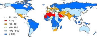
Predicted values of national annual median dilution factors. The median is a median across grid cells meeting inclusion criteria.
Across the globe, the differences in national annual dilution factors (and hence chemical concentrations) are extreme; for example, there are nearly 4 orders of magnitude between the annual median dilution factors in Canada (≈33 500) and Morocco (≈5). Most countries with the lowest median dilution factors (<10) are in North Africa and the Middle East. These areas tend to correspond to very arid regions (e.g., the Sahara) with few rivers. Population density can also play a significant role, as is the case in Belgium, where the annual dilution factor is among the lowest across the globe. Belgium is one of the countries in Europe with the highest population density: 343 cap/km2 in 2005 according to the United Nations Department of Economic and Social Affairs 39. Countries where low national dilution factors result in large part from high population densities include India, Belgium, the United Kingdom, and the Republic of Korea.
Most countries with high dilution factors are in North and South America, northern Europe, northern and eastern Asia, and Australia. The annual dilution factor for Australia seems unexpectedly high. Across Australia, only 10% of the cells have a river flow; thus, the dilution factor is not calculated in many parts of the country, in particular where population densities are relatively high and a low dilution factor might be expected. The national dilution factor for Australia, and many other countries, would therefore be much lower if the restriction on flow values was relaxed and cells with flow values of 0 m3/s were included in the calculation of the national statistics. A different type of problem is that associated with small countries as a result of the coarseness of the spatial resolution. At 0.5° resolution with an average cell size of 2250 km2, higher uncertainties arise when estimating runoff and, thus, river flow in catchments smaller than 25 000 km2 29. Although the concept of the dilution factor calculation remains valid when looking at smaller basins and therefore smaller countries such as Japan and the United Kingdom 40, a higher grid resolution would be more appropriate to reduce uncertainties in flow estimates 11.
Within-nation variability in dilution factors
National median values of annual dilution factor may be a useful starting point for comparison between countries of their potential exposure to down-the-drain chemicals. But the often unique spatial and temporal variabilities of dilution factor within a country must also be quantified because they can provide vital detail. The spatial variability of the annual dilution factor for some countries (tabulated values for all countries in Supplemental Data, Table S2) is captured in a box-and-whisker plot (Figure 2).
Figure 2.
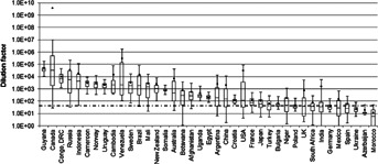
Spatial variability of the annual dilution factor between and within some countries. In each box-and-whisker plot, the box boundaries are the 25th and 75th percentiles, the line inside the box is the median, the whiskers are the 5th and 95th percentiles (where bottom whisker is missing, 0 < 5th percentile <1), and the dot is the mean. The dotted line represents a ratio of river flow to wastewater flow of 40, as recommended in engineering practice 38.
Significant differences occur within a country. There often is 1 order of magnitude between the 25th and the 75th percentiles (e.g., Australia, Cambodia, France); however, there are 3 orders of magnitude in Venezuela (≈330 and 141 680), and some countries have 2 orders of magnitude (e.g., United States, United Kingdom, Mexico, Argentina, Russia). These differences in dilution values essentially have 2 components: seasonal flow variations and demographic variations. These differences in dilution factors can reflect the variety of climates within a country (e.g., United States, from desert in Arizona to humid subtropical in Florida) or differences in population density (e.g., United Kingdom, low density in the highlands of Scotland, high density in southeast England). The mean dilution value can be particularly misleading; this is because of the possible wide range of dilution factor values within a country with an average often skewed by the highest values. This is clearly the case for Canada, the United States, Venezuela, the United Kingdom, and India (Figure 2). These important national differences emphasize the limitations of using a single value of annual dilution factor when assessing chemical exposure levels within a country.
Temporal (seasonal) variation can in some countries be the greatest source of variation in the dilution factor. Across the globe, the maximum monthly difference in median dilution factor can vary between 0 and 7 orders of magnitude in a country. Most countries with the highest order of magnitude (>7) between minimum and maximum monthly national dilution factors lie between the Tropic of Cancer and the Equator (e.g., Mali, Chad, Ethiopia, Thailand, and India). These countries tend to be in arid climates (northern Africa), where rivers can dry up, or tropical climates with dry winters (e.g., Thailand, India, and Cambodia), where monsoons can transform a small stream into a huge river. In contrast, most countries in temperate regions (e.g., France, United Kingdom, United States, and Paraguay) have the lowest temporal variability (between 0 and 2 orders of magnitude). Countries with a polar climate tend to have 2 to 4 orders of magnitude between the minimum and maximum monthly dilution factors; the temporal variation in these countries is a consequence of snow melt.
An example of this type of variability where countries/regions have a climate which can change from drought to torrential rains each year can be illustrated by flow regimes in the Ganges River (India) and the Changjang River (China) (Figure 3). The differences in flow, and hence dilution, between winter/spring and late summer/autumn is dramatic, changing more than 100-fold.
Figure 3.
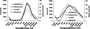
Temporal variability of mean monthly flow (measured and modeled at the gauging station) and median monthly dilution factor at the catchment and country scale for the river Ganges at Farakka in India (longitude = 87°92′, latitude = 24°83′) and the river Changjang at Datong in China (longitude = 117°61′, latitude = 30°76′). DF = dilution factor.
With this method, the temporal variability of the dilution factor is a reflection of the monthly variability in river flow as the population and per capita water use are assumed to be constant throughout the year. For these 2 large catchments, the modeled flows are in reasonable agreement with the observed flows. However, for the Changjang River, although the shape of the modeled hydrograph is reasonably similar, there is a temporal shift of about 1 mo. Such discrepancies are inevitable using global-scale hydrological models, but the essential observation is that the model has got the amount of flow available for dilution right in this case.
Using dilution factors
As an example, we can estimate the range of estrone (estrogenic female hormone) concentrations in rivers in Morocco and Canada using these dilution factor values. We will assume an excretion rate of 3.3 µg/d 7 and a daily per capita domestic water use for Morocco and Canada of, respectively, 96 L and 787 L 32,33 to estimate PECSEWAGE (Equation 1). No removal during wastewater treatment (F = 0, in Equation 2) is assumed, to provide a worst-case estimate. Applying Equation 1, the PECRIVER for Morocco is approximately equal to 5220 ng/L, 6 ng/L, and 1 ng/L when using, respectively, the 5th percentile, 50th percentile, and 95th percentile annual dilution factor (Supplemental Data, Table S2). For Canada, PECRIVER is approximately equal to 0.15 ng/L when using the 5th percentile annual dilution factor and less than 1 pg/L for both the median and the 95th percentile.
CONCLUSIONS
The principle of using available dilution as an indicator of potential national exposure to down-the-drain chemicals from the human population is a reasonable one. The method described in the present study is not claimed to be either unique or exclusive. There is no reason that other approaches to calculating flow and quantifying the local human population to provide dilution factors could not be equally, if not more, effective. We do not believe, however, that different methods would come to an entirely different conclusion. The present study hopefully can illustrate to a wide audience that the exposure to down-the-drain chemicals, and hence the experience of local aquatic wildlife, will be extraordinarily different between nations across the globe. Given the dramatic range of dilution factors, we would argue these are far more important determinants of chemical concentration in rivers than other variations in fate and behavior. These dilution factor values provide the means to estimate the possible range of in-river concentrations for any down-the-drain chemical where a per capita excretion, consumption, or even production value is available.
Despite a relatively crude approach, the present method revealed significant differences between nations with regard to the dilution they offer to down-the-drain chemicals. For the median annual dilution factor, there can be up to 4 orders of magnitude between countries and up to 3 orders of magnitude within a country. Temporal variability is also significant: within a country, the maximum monthly difference in dilution can vary between 0 and 9 orders of magnitude. Because of the great variability in dilution factors within many countries, comparing nations on the basis of a single dilution factor could be misleading.
Within every nation, depending on the location and time of year, there will be hot spots of chemical exposure; however, the present set of statistics helps define how widespread the issue could be. The present methodology provides a means of assessing where and when levels of exposure from down-the-drain chemicals might be of concern and, therefore, finer-resolution data and/or models applied or measurements taken.
It is hoped that the present approach might prove useful both to scientists and to regulators of nation-states, particularly in developing countries where few data sets exist, as a guide to potential exposures and, hence, risks from chemicals. The present methodology and data set may be combined with data such as consumption and degradation rates and simple water-quality principles to predict concentrations in rivers for individual down-the-drain chemicals. The present approach may be valuable to chemical companies as they consider new markets for their products. It also provides the basis for implementing future climate scenarios and therefore the means to assess the possible impact of climate change on dilution factors across the globe.
SUPPLEMENTAL DATA
Tables S1 and S2.
Figure S1. (80 KB PDF).
Supporting Information
All Supplemental Data may be found in the online version of this article.
Supporting Information.
REFERENCES
- 1.Jobling S, Williams R, Johnson A, Taylor A, Gross-Sorokin M, Nolan M, Tyler CR, van Aerle R, Santos E, Brighty G. Predicted exposures to steroid estrogens in UK rivers correlate with widespread sexual disruption in wild fish populations. Environ Health Perspect. 2006;114:32–39. doi: 10.1289/ehp.8050. [DOI] [PMC free article] [PubMed] [Google Scholar]
- 2.Tanaka H, Yakou Y, Takahashi A, Komori K, Okayasu Y. Evaluation of environmental estrogens in Japanese rivers. Proceedings Water Environment Federation Technical Exhibition and Conference; Atlanta, GA, USA: 2001. pp. 632–651. October 13–17, 2001. [Google Scholar]
- 3.Vethaak AD, Lahr J, Schrap SM, Belfroid AC, Rijs GBJ, Gerritsen A, de Boer J, Bulder AS, Grinwis GCM, Kuiper RV, Legler J, Murk TAJ, Peijnenburg W, Verhaar HJM, de Voogt P. An integrated assessment of estrogenic contamination and biological effects in the aquatic environment of The Netherlands. Chemosphere. 2005;59:511–524. doi: 10.1016/j.chemosphere.2004.12.053. [DOI] [PubMed] [Google Scholar]
- 4.Keller V. Risk assessment of “down-the-drain” chemicals: Search for a suitable model. Sci Total Environ. 2006;360:305–318. doi: 10.1016/j.scitotenv.2005.08.042. [DOI] [PubMed] [Google Scholar]
- 5.Johnson AC. Natural variations in flow are critical in determining concentrations of point source contaminants in rivers: An estrogen example. Environ Sci Technol. 2010;44:7865–7870. doi: 10.1021/es101799j. [DOI] [PubMed] [Google Scholar]
- 6.Osorio V, Marcé R, Pérez S, Ginebreda A, Cortina JL, Barceló D. Occurrence and modeling of pharmaceuticals on a sewage-impacted Mediterranean river and their dynamics under different hydrological conditions. Sci Total Environ. 2012;440:3–13. doi: 10.1016/j.scitotenv.2012.08.040. [DOI] [PubMed] [Google Scholar]
- 7.Williams RJ, Keller VD, Johnson AC, Young AR, Holmes MG, Wells C, Gross-Sorokin M, Benstead R. A national risk assessment for intersex in fish arising from steroid estrogens. Environ Toxicol Chem. 2009;28:446–446. doi: 10.1897/08-047.1. [DOI] [PubMed] [Google Scholar]
- 8.Bowden K, Brown SR. Relating effluent control parameters to river quality objectives using a generalized catchment simulation model. Water Sci Technol. 1984;16:197–206. [Google Scholar]
- 9.Feijtel T, Boeije G, Matthies M, Young A, Morris G, Gandolfi C, Hansen B, Fox K, Matthijs E, Koch V, Schroder R, Cassani G, Schowanek D, Rosenblom J, Holt M. Development of a geography-referenced regional exposure assessment tool for European rivers—GREAT-ER. J Hazard Mater. 1998;61:59–65. [Google Scholar]
- 10.Vörösmarty CJ, McIntyre PB, Gessner MO, Dudgeon D, Prusevich A, Green P, Glidden S, Bunn SE, Sullivan CA, Liermann CR, Davies PM. Global threats to human water security and river biodiversity. Nature. 2010;467:555–561. doi: 10.1038/nature09440. [DOI] [PubMed] [Google Scholar]
- 11.Keller VDJ, Rees HG, Fox KK, Whelan MJ. A new generic approach for estimating the concentrations of down-the-drain chemicals at catchment and national scale. Environ Pollut. 2007;148:334–342. doi: 10.1016/j.envpol.2006.10.048. [DOI] [PubMed] [Google Scholar]
- 12.Keller VDJ, Whelan MJ, Rees HG. A global assessment of chemical effluent dilution capacities from a macro-scale hydrological model. In: Demuth S, Gustard A, Planos E, Scatena F, Servat E, editors. Climate Variability and Change—Hydrological Impacts. Wallingford, UK: International Association of Hydrological Sciences; 2006. pp. 586–590. IAHS Publication 308. [Google Scholar]
- 13.Arnell NW. A simple water balance model for the simulation of streamflow over a large geographic domain. J Hydrol. 1999;217:314–335. [Google Scholar]
- 14.Nijssen B, O'Donnell GM, Lettenmaier DP, Lohmann D, Wood EF. Predicting the discharge of global rivers. J Climate. 2001;14:3307–3323. [Google Scholar]
- 15.Vörösmarty CJ, Federer CA, Schloss AL. Potential evaporation functions compared on US watersheds: Possible implications for global-scale water balance and terrestrial ecosystem modeling. J Hydrol. 1998;207:147–169. [Google Scholar]
- 16.Alcamo J, Doll P, Henrichs T, Kaspar F, Lehner B, Rosch T, Siebert S. Development and testing of the WaterGAP 2 global model of water use and availability. Hydrological Sciences Journal. 2003;48:317–337. [Google Scholar]
- 17.Döll P, Kaspar F, Lehner B. A global hydrological model for deriving water availability indicators: Model tuning and validation. J Hydrol. 2003;270:105–134. [Google Scholar]
- 18.Abdulla FA, Lettenmaier DP. Application of regional parameter estimation schemes to simulate the water balance of a large continental river. J Hydrol. 1997;197:258–285. [Google Scholar]
- 19.Arnell NW. Climate change and global water resources: SRES emissions and socio-economic scenarios. Global Environ Chang. 2004;14:31–52. [Google Scholar]
- 20.Beek TAD, Voss F, Floerke M. Modelling the impact of global change on the hydrological system of the Aral Sea basin. Phys Chem Earth. 2011;36:684–695. [Google Scholar]
- 21.Fekete BM, Vörösmarty CJ, Grabs W. High-resolution fields of global runoff combining observed river discharge and simulated water balances. Global Biogeochem Cy. 2002;16:1042. [Google Scholar]
- 22.Legates DR, Willmott CJ. Mean seasonal and spatial variability in gauge-corrected, global precipitation. Int J Climatol. 1990;10:111–127. [Google Scholar]
- 23.Legates DR, Willmott CJ. Mean seasonal and spatial variability in global surface air-temperature. Theor Appl Clim. 1990;41:11–21. [Google Scholar]
- 24.Food and Agriculture Organization/United Nations Educational, Scientific and Cultural Organization. Carouge, Switzerland: 1986. Gridded FAO/UNESCO soil units, UNEP/GRID, FAO soil map of the world in digital form. [Google Scholar]
- 25.Edwards M. Boulder, CO, USA: National Oceanic and Atmospheric Administration, National Geophysical Data Center; 1988. Data announcement 88-MGG-02: Digital relief of the surface of the earth. [Google Scholar]
- 26.Olson JS. Boulder, CO, USA: National Oceanic and Atmospheric Administration National Geophysical Data Center; 1992. World ecosystems. Digital raster data on global geographic (lat/long) 180 × 360 and 1080 × 2160 grids. [Google Scholar]
- 27.Melillo JM, McGuire AD, Kicklighter DW, Moore B, Vorosmarty CJ, Schloss AL. Global climate change and terrestrial net primary production. Nature. 1993;363:234–240. [Google Scholar]
- 28.Global Runoff Data Centre. The German Federal Institute of Hydrology (BfG) 2013. cited 2013 25 July]. Available from: http://www.bafg.de/GRDC/EN/Home/homepage_node.html.
- 29.Vörösmarty CJ, Fekete BM, Meybeck M, Lammers RB. Geomorphometric attributes of the global system of rivers at 30-minute spatial resolution. J Hydrol. 2000;237:17–39. [Google Scholar]
- 30.Keller V, Rees HG. Wallingford, UK: Report to Unilever; 2005. GLODIF: Global scale estimation of dilution factors for down the drain chemicals in surface waters—Final report. [Google Scholar]
- 31.Center for International Earth Science Information Network, Centro Internacional de Agricultura Tropical. Palisades, NY, USA: Socioeconomic Data and Applications Center, Columbia University; 2005. Gridded Population of the World, Version 3 (GPWv3) [Google Scholar]
- 32.Gleick P. The World's Water 2008–2009: The Biennial Report on Freshwater Resources. Washington, DC: Island Press; 2009. [Google Scholar]
- 33.Food and Agriculture Organization. AQUASTAT database. 2000. cited 2013 July 25]. Available from: http://www.fao.org/nr/water/aquastat/main/index.stm.
- 34.World Resource Institute. Actual renewable water resources: Per capita. 2007. cited 2011 August 18]. Available from: http://earthtrends.wri.org/searchable_db/index.php?theme=2.
- 35.Organisation for Economic Co-operation and Development. Environmental indicators, modelling and outlooks. OECD Environmental Data Compendium. 2008. cited 2013 July 25]. Available from: http://www.oecd.org/env/indicators-modelling-outlooks/oecdenvironmentaldatacompendium.htm.
- 36.Keshavarzi AR, Sharifzadeh M, Hahighi AAK, Amin S, Keshtkar S, Bamdad A. Rural domestic water consumption behavior: A case study in Ramjerd area, Fars Province, Iran. Water Res. 2006;40:1173–1178. doi: 10.1016/j.watres.2006.01.021. [DOI] [PubMed] [Google Scholar]
- 37.Sandiford P, Gorter AC, Orozco JG, Pauw JP. Determinants of domestic water-use in rural Nicaragua. J Trop Med Hyg. 1990;93:383–389. [PubMed] [Google Scholar]
- 38.Gupta RS. Hydrology and Hydraulic Systems. 3rd ed. Long Grove, IL, USA: Waveland Press; 2008. [Google Scholar]
- 39.United Nations Department of Economic and Social Affairs. New York, NY, USA: 2008. 2005 Demographic Yearbook. [Google Scholar]
- 40.Johnson AC, Yoshitani J, Tanaka H, Suzuki Y. Predicting national exposure to a point source chemical: Japan and endocrine disruption as an example. Environ Sci Technol. 2011;45:1028–1033. doi: 10.1021/es103358t. [DOI] [PubMed] [Google Scholar]
Associated Data
This section collects any data citations, data availability statements, or supplementary materials included in this article.
Supplementary Materials
Supporting Information.