A minimal model of protein–protein binding affinities

Abstract

A minimal model of protein–protein binding affinity that takes into account only two structural features of the complex, the size of its interface, and the amplitude of the conformation change between the free and bound subunits, is tested on the 144 complexes of a structure-affinity benchmark. It yields K_d values that are within two orders of magnitude of the experiment for 67% of the complexes, within three orders for 88%, and fails on 12%, which display either large conformation changes, or a very high or a low affinity. The minimal model lacks the specificity and accuracy needed to make useful affinity predictions, but it should help in assessing the added value of parameters used by more elaborate models, and set a baseline for evaluating their performances.

Introduction

Relating the binding affinity of two proteins to the structure of their complex has been an active field of research for many years.^1–3 Current models of the structure/affinity relationship may take into account the physical chemical properties of the interface between subunits, and attempt to reproduce the energetics of their interaction, a very difficult task when conformation changes accompany binding. Alternatively, they may rely on empirical score functions developed for protein–protein docking, or derived by machine-learning procedures from sets of data collected from the literature. Such models can also incorporate biological information on the conservation of the protein sequence or the effect of point mutations. They have many variable parameters, and their assessment has been done in different ways on different test sets, making a comparison difficult.^4–9 Moreover, the datasets used for training and testing the models have often been small and of poor quality, prompting Kastritis et al.¹⁰ to assemble a validated Structure-Affinity Benchmark (SAB) designed for this purpose.

Here, we present a model with only two features: the size of the interface between subunits and the amplitude of the conformation change between the free proteins and the complex. When applied to SAB, it yields acceptable affinity predictions for 126 of the 144 complexes in the SAB. The model fails on eight complexes that display large conformation changes, four enzyme-inhibitor complexes with picomolar affinity, and six other complexes that are much less affine than predicted. It also fails to explain how the specific interactions represented in the SAB can compete with the many contacts of no biological relevance that result from random collisions in the cell. Conversely, it correctly models the affinity of antigen-antibody complexes and of enzyme complexes with protein substrates or regulatory chains, and it reproduces the effect on affinity of small and medium amplitude conformation changes. Thus, the two-feature model sets a baseline to assess the value of other parameters in prediction schemes that can take into account the detailed atomic nature of the interactions and the conformation changes, the physical chemistry of protein–protein interfaces, their conservation in evolution, and the effect on affinity of pH and other environmental factors.

The Model

The SAB, designed to develop and test structure-based models of protein–protein binding affinities,¹⁰ associates equilibrium constants (K_d) measured in solution, and the derived Gibbs free energies of dissociation (ΔG_d), to entries of the Protein Data Bank that describe 144 protein–protein complexes and their free components. The SAB also reports the conditions under which K_d has been determined, and it quotes two geometric quantities computed on the atomic coordinates: ΔASA, the area of the protein surface buried at the interface of the complex; iRMSD, the root-mean-square displacement of the Cα atoms of interface residues between the bound and unbound structures. ΔASA measures the size of the protein surfaces in contact, iRMSD, the amplitude of the conformation change accompanying the interaction.

A larger ΔASA implies that more protein atoms become desolvated in the complex, and more noncovalent interactions are made across the interface. This is expected to improve affinity, whereas, a larger iRMSD implies more costly conformation changes, and lesser affinity. This is confirmed in the SAB: ΔG_d exhibits a weak negative correlation with iRMSD (R = −0.26), and a positive correlation (R = 0.59) with ΔASA in complexes displaying small changes, but these correlations vanish in complexes that display large changes.¹⁰ The free energy cost of conformation changes depends on details of both the bound and the unbound atomic structures, yet small changes may be amenable to a harmonic approximation similar to the one used in Gaussian networks. Thus, one may write:

1

The 144 entries of the SAB comprise 135 cognate and nine noncognate complexes. We distribute the cognate complexes into three categories depending on the amplitude of the conformation change: 75 small (iRMSD < 1.1 Å), 27 medium (1.1–1.5 Å), and 33 large (iRMSD > 1.5 Å). The docking benchmark from which the SAB was derived classifies its entries in a similar way according to iRMSD: easy (rigid body), medium difficulty, or difficult to dock.¹¹ The values of α, β, and γ cited in the legend of Figure 1 are issued from a least-square fit of data on complexes of the small change category after removing six outliers discussed below. The values of ΔG_calc obtained with those parameters are listed in Supporting Information Table S1.

Figure 1.

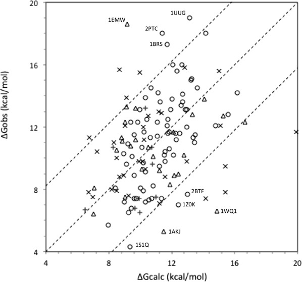
Comparing calculated and experimental binding energies. ΔG_d from the SAB¹⁰ is plotted against ΔG_calc, derived from Eq. (1) with parameters: α = 6.1 kcal mol⁻¹, β = 3.8 cal mol Å⁻², γ = −1.7 kcal mol Å⁻², d_max = 1.5 Å. The dashed lines parallel to the diagonal correspond to ΔG_calc = ΔG_d ± 4.2 kcal mol⁻¹. Labels: (o) small conformation changes (iRMSD < 1.1 Å); (Δ) medium changes (1.1–1.5 Å); (x) large changes (>1.5 Å); (+) noncognate complexes.

Table1 reports statistics on the experimental values of ΔG_d and their fit by Eq. (1). Relative to the standard deviation of ΔG_d, the RMS discrepancy ΔΔG_rms indicates that the two features of the model account for about half of the variance of the 69 data used to derive the coefficients. ΔG_d and ΔG_calc are significantly correlated (R = 0.63 excluding outliers, which yields a P-value below 10⁻⁶), and the absolute discrepancy |ΔΔG| is less than 4.2 kcal mol⁻¹, meaning that K_d is predicted to within a factor of 10³, in which case we consider that Eq. (1) makes an acceptable affinity prediction. These 69 complexes yield points in between the dotted lines of Figure 1.

Table I.

Fitting Experimental ΔG_d Values

Category of complex		ΔGd (kcal mol−1)		ΔGcalc fit to ΔGd
	Number	Mean	s.d.	Outliers	ΔΔGrms (kcal mol−1)	Correl. coeff. R
Conformation change (iRMSD)
Small (<1.1 Å)	75	11.4	3.1	6	2.6	0.55
Excluding outliers	69	11.3	2.9	–	2.1	0.63
Medium (1.1–1.5 Å)	27	10.6	2.8	4	3.5	0.38
Large (>1.5 Å)	33	10.7	2.6	8	3.6	0.16
Functional
A: Antigen–Antibody	17	12.4	1.7	0	1.9
EI: Enzyme-inhibitor	36	13.8	2.3	8	2.3*
EX: Other enzyme complexes	20	9.2	1.9	1	2.2*
O: Other complexes	62	9.7	2.4	9	2.0*
NC: Noncognate	9	8.8	2.4	0	2.4
All	144	10.9	2.9	18	3.0	0.32

ΔG_d is from the SAB¹⁰, ΔG_calc, from Eq. (1) with the parameters cited in the legend of Figure 1; ΔΔG is their difference; s.d.: standard deviation of ΔG_d; ΔΔG_rms: root-mean-square value of ΔΔG. |ΔΔG| > 4.2 kcal mol⁻¹ defines outliers; (^*) excluding outliers.

With the same coefficients, Eq. (1) also makes acceptable affinity predictions for 23 of the 27 complexes of the medium change category, but the correlation is poor (R = 0.38). Above iRMSD = 1.5 Å, the harmonic approximation breaks down, and ΔASA, which is measured only on the complex, no longer represents the area of the protein surface buried upon association.¹² As a result, Eq. (1) underestimates ΔG_d for most of the 33 complexes of the large change category. Nevertheless, it returns acceptable predictions for 25 of them if d_max is set to 1.5 Å, which effectively limits to 3.8 kcal mol⁻¹ the cost of the conformation change. That cost is negligible (less than 0.1 kcal mol⁻¹) when iRMSD is below 0.25 Å, which represents errors of atomic coordinates rather than an actual change.

Functional Classes, Outliers, and Noncognate Complexes

Table1 also reports statistics on the SAB complexes distributed according to function. Class A comprises 17 antigen-antibody complexes. Equation (1) makes acceptable affinity predictions for all, but the mean ΔG_d value is a better predictor, as the standard deviation is less than ΔΔG_rms. Moreover, Eq. (1) underestimates ΔG_d by an average of about 1 kcal mol⁻¹ in class A, and changing the α parameter by that amount makes the prediction more accurate.

Equation (1) also tends to underestimate ΔG_d in class EI (enzyme inhibitor), but then, ΔΔG exceeds 4.2 kcal mol⁻¹ for eight complexes, which yield the eight points above the dashed line in the top left quadrant of Figure 1. Two of those outliers involve a metal bond (1JIW, 4CPA). In four other, which display a very high (subpicomolar) affinity (1EMV, 1BRS, 1UUG, 2O3B), the inhibitor takes the place of a DNA or RNA substrate, and it forms with the enzyme strong electrostatic interactions more common in protein–nucleic acid than protein–protein complexes. Another very high affinity outlier is the trypsin-pancreatic inhibitor complex (2PTC), where the charge carried by Lys15 of the inhibitor accounts for a large fraction of the binding energy; in that case, ΔG_calc is close to the value observed with the Met15 mutant.¹³ Equation (1) also makes acceptable predictions for the less affine noncognate counterparts (2WPT, 1AY7, 1CBW) of those outliers.

Class EX comprises 20 complexes of enzymes with protein substrates or regulatory chains, which are much less affine than inhibitors. Equation (1) makes acceptable predictions for all but one that displays a large conformation change (1JMO). But here again, the standard deviation of ΔG_d is less than ΔΔG_rms, and thus, the mean value in the class is a better predictor.

Class O is very diverse. Many of its 62 complexes undergo large conformation changes, often related to allosteric effects, and their affinity is comparatively low. Equation (1) makes acceptable affinity predictions for 53, and overestimates the affinity of the other 9, which yield the 9 points in the lower right quadrant of Figure 1. Four display large conformation changes that may cost much more than the 3.8 kcal mol⁻¹ maximum set in Eq. (1). The low affinity of the others is not predicted by the model.

Equation (1) makes acceptable affinity predictions for all the nine noncognate complexes of the SAB. In two cases (2AQ3 and 2PCB), it correctly predicts the loss in ΔG_d relative to the cognate complex, but the predicted loss is 3–7 kcal mol⁻¹ less than reported in Table 2 of Kastritis et al.¹⁰ for the other seven cognate/noncognate pairs.

Discussion

Modeling affinity

The minimal model represented by Eq. (1) takes into account the size of the interface between the subunits and the effect of conformation changes on affinity, but it ignores altogether the chemical nature of the protein surfaces and the physics of their interactions, which a more elaborate model can represent in a variety of ways with additional parameters. As a test, we broke ΔASA into a nonpolar (carbon containing) and a polar (N/O-containing) component. This adds only one parameter, but brings no significant improvement to the fit, probably because the two components are tightly correlated to ΔASA. As the model stands, the overall quality of its predictions shown in Table1 is comparable to that of several prediction schemes that have many more adjustable parameters.^4–9 It fails in three cases: (a) large conformation changes; (b) enzyme-inhibitor complexes much more affine than predicted; and (c) “other” complexes less affine than predicted. Fitting (a)-type outliers will require accurate estimates of the free energy cost of conformation changes, still a major endeavor. Electrostatic interactions, including those that occur far from the interface,¹⁴ play a major role in (b)-type outliers. Whereas empirical or residue-level potentials seem unable to reproduce the very high affinity of the enzyme-inhibitor complexes, they should be amenable to computational methods that rely on detailed atomic structures.¹⁵ This may also apply to some of the (c)-type outliers, but the origin of their low affinity is probably different in each.

Equation (1) predicts ΔG_d to within 4.2 kcal mol⁻¹, and K_d to within three orders of magnitude, for 88% of the SAB complexes. In comparison, the recent affinity prediction schemes of Moal et al.⁵ and Vreven et al.⁶ achieve that accuracy on respectively 91 and 92%. This allows placing the complexes in the right high/medium/low affinity class,¹⁰ but most applications require a much better accuracy. To reach one order of magnitude, the environment must be modeled along with the proteins, because K_d values measured by different methods or under different conditions typically differ by a factor of 2–10. The pH of most of the measurements reported in the SAB is in the range 5.5–8.5. Changing it by two units in that range can change K_d more than 10-fold. Thus, modeling pH effects is essential, which in turn implies making accurate pK_a predictions for all protein groups titrating in the range 4.5–9.5.

An accuracy of two orders of magnitude in K_d, or |ΔΔG| = 2.8 kcal mol⁻¹, is a more realistic goal for affinity prediction methods. Equation (1) reaches that goal for 97 or 67%, of the 144 complexes in the SAB. Moal et al.⁵ and Vreven et al.⁶ do significantly better (about 80%), but taking the mean value of ΔG_d in the class remains the best choice for complexes of class A and EX, as all but one antigen-antibody complexes, and all but three enzyme complexes with protein substrates or regulatory chains, have a K_d that differs by factors less than 100 from the log-average of the class.

Modeling specificity

Modeling specificity can be as important as affinity. In the SAB, specificity may be assessed on pairs of cognate and noncognate complexes, similar in structure but different in affinity. The minimal model does poorly, because Eq. (1) returns similar values for the two members of a pair, and it underestimates the affinity of the cognate member while correctly predicting that of the noncognate. Other models encounter the same problem in spite of having more parameters.

An essential aspect of specificity is not represented in the SAB, and it has been ignored by most modeling schemes. In a cell, biologically relevant interactions compete with random pairs that form all the time as molecules collide. The affinity of a random pair should be modeled and found to be much lower. In docking simulations, with only two proteins present, the native pose typically competes with 10⁵ nonnative poses. Their binding energies are distributed according to a random energy model,¹⁶ and the average value ΔG_random has to be at least 7 kcal mol⁻¹ less than for the native pose to populate the latter. In the much more diverse environment of a cell, ΔG_random should probably be negative (i.e., K_random >1 M), for functional interactions with a micromolar K_d to survive the competition. Instead, Eq. (1) yields ΔG_calc values similar to the binding energy of some of the SAB complexes if ΔASA is set to 200 or 400 Ų, which random docking typically achieves. This simple test, which the minimal model fails to pass, ought to be applied to all affinity prediction schemes.

Methods

K_d, ΔG_d, ΔASA, and iRMSD values were taken from Table S1 of Kastritis et al.¹⁰ The K_d of 1NSN, 1IQD, and 1UUG, given as <X in Table S1, was arbitrarily set to X/5. Other data in the text were obtained from Table S8 of Moal et al.⁵ and Table S6 of Vreven et al.⁶

Supporting Information

Additional Supporting Information may be found in the online version of this article.

Supplementary Information Table 1.

References

- Horton N, Lewis M. Calculation of the free energy of association for protein complexes. Protein Sci. 1992;1:169–181. doi: 10.1002/pro.5560010117. [DOI] [PMC free article] [PubMed] [Google Scholar]
- Kastritis PL, Bonvin AM. Molecular origins of binding affinity: seeking the Archimedean point. Curr Opin Struct Biol. 2013;23:868–877. doi: 10.1016/j.sbi.2013.07.001. [DOI] [PubMed] [Google Scholar]
- Moal IH, Moretti R, Baker D, Fernández-Recio J. Scoring functions for protein–protein interactions. Curr Opin Struct Biol. 2013;23:862–867. doi: 10.1016/j.sbi.2013.06.017. [DOI] [PubMed] [Google Scholar]
- Kastritis PL, Bonvin AM. Are scoring functions in protein–protein docking ready to predict interactomes? Clues from a novel binding affinity benchmark. J Proteome Res. 2010;9:2216–2225. doi: 10.1021/pr9009854. Erratum in: J Proteome Res (2011) 10:921–922. [DOI] [PubMed] [Google Scholar]
- Moal IH, Agius R, Bates PA. Protein–protein binding affinity prediction on a diverse set of structures. Bioinformatics. 2011;27:3002–3009. doi: 10.1093/bioinformatics/btr513. [DOI] [PubMed] [Google Scholar]
- Vreven T, Hwang H, Pierce BG, Weng Z. Prediction of protein–protein binding free energies. Protein Sci. 2012;21:396–404. doi: 10.1002/pro.2027. [DOI] [PMC free article] [PubMed] [Google Scholar]
- Pallara C, Jiménez-García B, Pérez-Cano L, Romero-Durana M, Solernou A, Grosdidier S, Pons C, Moal IH, Fernandez-Recio J. Expanding the frontiers of protein–protein modeling: from docking and scoring to binding affinity predictions and other challenges. Proteins. 2013;81:2192–2200. doi: 10.1002/prot.24387. [DOI] [PubMed] [Google Scholar]
- Yan Z, Guo L, Hu L, Wang J. Specificity and affinity quantification of protein–protein interactions. Bioinformatics. 2013;29:1127–1133. doi: 10.1093/bioinformatics/btt121. [DOI] [PubMed] [Google Scholar]
- Luo J, Guo Y, Zhong Y, Ma D, Li W, Li M. A functional feature analysis on diverse protein–protein interactions: application to the prediction of binding affinity. J Comput Aided Mol Des. 2014;28:619–629. doi: 10.1007/s10822-014-9746-y. [DOI] [PubMed] [Google Scholar]
- Kastritis PL, Moal IH, Hwang H, Weng Z, Bates PA, Bonvin AM, Janin J. A structure-based benchmark for protein–protein binding affinity. Protein Sci. 2011;20:482–491. doi: 10.1002/pro.580. [DOI] [PMC free article] [PubMed] [Google Scholar]
- Hwang H, Vreven T, Janin J, Weng Z. Protein–protein docking benchmark version 4.0. Proteins. 2010;78:3111–3114. doi: 10.1002/prot.22830. [DOI] [PMC free article] [PubMed] [Google Scholar]
- Chakravarty D, Guharoy M, Robert CH, Chakrabarti P, Janin J. Reassessing buried surface areas in protein–protein complexes. Protein Sci. 2013;22:1453–1457. doi: 10.1002/pro.2330. [DOI] [PMC free article] [PubMed] [Google Scholar]
- Helland R, Otlewski J, Sundheim O, Dadlez M, Smalås AO. The crystal structures of the complexes between bovine beta-trypsin and ten P1 variants of BPTI. J Mol Biol. 1999;287:923–942. doi: 10.1006/jmbi.1999.2654. [DOI] [PubMed] [Google Scholar]
- Kastritis PL, Rodrigues JP, Folkers GE, Boelens R, Bonvin AM. Proteins feel more than they see: fine-tuning of binding affinity by properties of the non-interacting surface. J Mol Biol. 2014;426:2632–2652. doi: 10.1016/j.jmb.2014.04.017. [DOI] [PubMed] [Google Scholar]
- Koehl P. Electrostatics calculations: latest methodological advances. Curr Opin Struct Biol. 2006;16:142–151. doi: 10.1016/j.sbi.2006.03.001. [DOI] [PubMed] [Google Scholar]
- Bernauer J, Poupon A, Azé J, Janin J. A docking analysis of the statistical physics of protein–protein recognition. Phys Biol. 2005;2:S17–S23. doi: 10.1088/1478-3975/2/2/S02. [DOI] [PubMed] [Google Scholar]
Associated Data
This section collects any data citations, data availability statements, or supplementary materials included in this article.
Supplementary Materials