Measures of discrimination for latent group-based trajectory models

Abstract

In clinical research, patient care decisions are often easier to make if patients are classified into a manageable number of groups based on homogeneous risk patterns. Investigators can use latent group-based trajectory modeling to estimate the posterior probabilities that an individual will be classified into a particular group of risk patterns. Although this method is increasingly used in clinical research, there is currently no measure that can be used to determine whether an individual’s group assignment has a high level of discrimination. In this study, we propose a discrimination index and provide confidence intervals of the probability of the assigned group for each individual. We also propose a modified form of entropy to measure discrimination. The two proposed measures were applied to assess the group assignments of the longitudinal patterns of conduct disorders among young adolescent girls.

1. Introduction

Latent group-based trajectory models [10] have increasing been used to identify distinct trajectory patterns in longitudinal data. One of the main advantages of latent group-based trajectory models is that they allow for the discovery of subgroup behaviors for a population with unobserved heterogeneity across time. For example, if a treatment is administered to a population of patients, there may be distinct response subgroups within that population. One group may respond favorably to the treatment while another group responds negatively, and maybe a third group does not respond at all. Discovering these unobserved patterns of behavior could be extremely useful. Clinicians may target more individual-based therapies based on a patient’s profile if they believe a patient falls into one of these subgroups. It is worth noting that a latent group-based trajectory model is a special case of growth mixture models [11]. Latent group-based trajectory models assume a linear model to fit longitudinal trajectories over time, while growth mixture models assume a linear mixed model with possibly random intercepts and random slopes to fit the trajectories. These random components allow individuals within the same trajectory group to vary around the mean group trajectory.

To assess how well a model fits with the data, several goodness-of-fit measures have been proposed for the latent group-based trajectory models. Nagin [10] developed two measures to assess the model adequacy: use of the average posterior probability of assignment (APPA) and use of the odds of correct classification (OCC). Berkhof et al. [2] proposed a discrepancy measure to assess the model fit. Lindsay and Roeder [8] developed gradient-based diagnostic measures for continuous outcomes and residual plots for discrete outcomes. Agresti [1] proposed the use of G² statistic to measure the absolute model fit.

For analysis using latent group-based trajectory modeling, we need to first assume a certain number of latent groups and then estimate the best trajectory curve for each group via appropriate inference procedures. Several model selection techniques are available to decide what the number of latent groups should be chosen to best fit the data. One obvious candidate, the likelihood ratio test, cannot be used. It does not have the usual large sample chi-square distribution properties due to the class probability parameter being at the border of its admissible space [12]. Commonly used model selection techniques include Akaike information criteria (AIC), Bayesian information criteria (BIC), and the bootstrap likelihood ratio test (BLRT). Simulations by Nylund et al. [11] showed that BIC and BLRT outperformed AIC and suggested that BIC and BLRT need to be compared together.

Although there are several methods to test the goodness-of-fit for latent group-based trajectory models, currently, there is no measure of discrimination to check the confidence of an individual being assigned to a certain group. This can be particularly troubling if treatment regimens are determined by an individual’s group assignment. For example, in the two-group scenario, an individual may be in group one with a probability of 0.98 and in group two with a probability of 0.02. This individual’s group assignment has a high level of discrimination and is assigned to group one. However, another individual may have a group one probability of 0.52 and a group two probability of 0.48. This individual is also assigned to group one even though his or her group membership has a poor level of discrimination. Recognizing this ambiguity may play a large role in how clinicians decide to treat individuals. In this paper, we propose two measures to evaluate discrimination, and they can be used along with the goodness-of-fit techniques to evaluate latent group-based trajectory models.

In Section 2, we introduce the notation and revisit the latent-group trajectory models. In Section 3, we introduce the first discrimination measure by modifying entropy, and the second discrimination measure and its corresponding variance estimator based on the posterior probabilities of group membership. In Section 4, we conduct simulations to assess the performance of our discrimination measures. In Section 5, we apply the proposed measures to a longitudinal study for the development of conduct disorders among young girls. The paper is concluded in Section 6.

2. Notation and model

The latent group-based trajectory model [10] is a mixture of two components. The group membership is modeled via a multinomial regression. The longitudinal trajectories, conditional on a given group membership, are modeled via a linear model. The general form of the log-likelihood can be specified as follows:

$$\mathit{log}(L)=\sum _{i=1}^n\mathit{log}\left(\sum _{j=1}^{J}Pr(X_i=j\mid Z_i=z_i)Pr(Y_i=y_i\mid X_i=j,W_i=w_i)\right)=\sum _{i=1}^n\mathit{log}\left(\sum _{j=1}^J{\pi }_{ij}Pr(Y_i=y_i\mid X_i=j,W_i=w_i)\right)$$ (1)

where Z represents time-independent covariates, W represents time-independent or time-dependent covariates, Y represents an individual’s longitudinal profile, and X is a random variable. For subject i, the first term of (1) represents the probability of belonging to group membership j,

$${\pi }_{ij}=Pr(X_i=j\mid Z_i=z_i)=\frac{exp({\theta }_j+{\lambda }_j^T{z}_i)}{{\sum }_{l=1}^{J}exp({\theta }_l+{\lambda }_l^T{z}_i)}.$$

This logistic function models the probability of an individual belonging to a certain group. The second term of (1) represents the probability of the longitudinal outcomes Y_i given the group membership j,

$$\mathit{MVN}({\mu }_j,{\mathrm{\sum }}_j)=Pr(Y_i=y_i\mid X_i=j,W_i=w_i)=\frac{1}{{(2\pi )}^{\frac{t}{2}}{\mid {\mathrm{\sum }}_j\mid }^{\frac{1}{2}}}exp\left\{-\frac{1}{2}{(y_i-{\mu }_j)}^T{\mathrm{\sum }}_j^{-1}(y_i-{\mu }_j)\right\}.$$

Mean μ_j can be specified as a polynomial function of time with the form

$${\mu }_j={\beta }_0+{\beta }_1^{T}t+{\beta }_2^T{t}^2+{\beta }_3^T{t}^3+\dots$$

The mean trajectories may also depend on covariates W. When there are only two latent groups involved, the log likelihood can be simplified as the form:

$$log(L)=\sum _{i=1}^{n}log\{{\pi }_i\mathit{MVN}({\mu }_1,{\mathrm{\sum }}_1)+(1-{\pi }_i)\mathit{MVN}({\mu }_2,{\mathrm{\sum }}_2)\},$$

where MVN (μ, Σ) is a multivariate normal density with mean vector μ and variance-covariance matrix Σ. The five parameters that need to be estimated from this model are π_i, μ₁, Σ₁, μ₂, and Σ₂. Maximization of the log likelihood function can be done by using the quasi-Newton procedures. The estimated parameters are necessary for calculating the posterior probability of an individual being in a particular group. The group-based model assumes conditional independence; within each group, an individual’s longitudinal value is not correlated with its previous time point value [10]. Nagin notes that while this is a strong assumption, random effects models assume conditional independence at the individual level, and the group-based model makes no assumptions regarding the independent and identical distribution of of such random effects [10].

3. Discrimination statistics

Once parameter estimates are obtained, posterior probabilities can be calculated. Using Bayes rule, the posterior probability of individual i belonging to group j given his or her longitudinal trajectory is

$$\widehat{P}r(X_i=j\mid Y_i)=\frac{\widehat{P}r(Y_i\mid X_i=j){\widehat{\pi }}_{ij}}{{\sum }_{j=1}^J\widehat{P}r(Y_i\mid X_i=j){\widehat{\pi }}_{ij}}.$$

For example, if there are 2 groups (j = 2), each individual will have a probability of being in group 1 and a probability of being in group 2. The group assignment depends on the largest of the two posterior probabilities. As mentioned above, the level of discrimination plays no part in group assignment. Therefore, individuals whose posterior probabilities are highly ambiguous are still assigned to groups just as individuals whose posterior probabilities are highly discriminated are.

Entropy is a statistic used to measure the amount of information or the degree of classification uncertainty in various fields including latent-class analysis. Individual-level entropy [4] is defined as

$$EN=-\sum _{J=1}^J{\widehat{p}}_{j}log({\widehat{p}}_j),$$

where p̂_j is the estimate of the individual’s posterior probability of being in group j. Larger value of entropy indicates higher level of uncertainty in discrimination. Therefore, subjects who are poorly discriminated should have higher values of entropy than subjects who are well discriminated. One important caveat is that entropy is based on all posterior probabilities, but for group assignment, we are most interested in the gap between the highest posterior probability and the second highest posterior probability. For example, in a four group scenario, if a subject’s posterior probabilities are 0.25 for each group, discrimination will be poor and entropy high. However, if the posterior probabilities are 0.4, 0.2, 0.2, and 0.2, entropy will still be relatively high even though we may confidently be able to assign the subject to the group with posterior probability 0.4. Since it is essentially the leading two posterior probabilities that determine discrimination status, we propose a modification of the entropy measure by considering only these leading two posterior probabilities. The modified entropy has the form

$${EN}_m=-\{{\widehat{p}}_{(1)}log({\widehat{p}}_{(1)})+{\widehat{p}}_{(2)}log({\widehat{p}}_{(2)})\},$$ (2)

where p̂(1) and p̂(2) are the largest and the second largest posterior probabilities, respectively.

To build up our second discrimination measure, we will first construct a confidence interval around the maximum posterior probability. An individual’s discrimination will then be determined by whether the confidence interval of the maximum posterior probability contains the parameter (p̂(1) + p̂(2))/2. Another way to represent this is

$${\widehat{p}}_{(1)}-z_{a/2}\frac{sd}{\sqrt{n}}<\frac{p_{(1)}+p_{(2)}}{2}<{\widehat{p}}_{(1)}+z_{\alpha /2}\frac{sd}{\sqrt{n}},$$ (3)

where $sd/\sqrt{n}$ represents the standard error of the estimator p̂(1). Note that we assume normality in the calculation of the confidence interval. Simply put, if the average of the two maximum posterior probabilities is contained within the confidence interval of of the maximum posterior probability, we consider the discrimination decision adequate.

We considered several methods to estimate the variance of posterior probabilities of group membership. One technique was calculating the distribution of the order statistic of the posterior probabilities. However, this would necessitate knowing how the probabilities are distributed. Another method considered was using the bootstrap technique [5], but it is very computationally intensive. We will adopt the method proposed by Menses et al. [9] to estimate the variance of the posterior probabilities. They derived the variance estimator using the delta method,

$$\mathit{Var}({\widehat{p}}_{(1)})=\mathit{Var}\{Pr(X_i=j\mid Y_i)\}\approx {\left\{\frac{\partial Pr(X_i=j\mid Y_i)}{\partial y}\right\}}^T\mathit{Var}(Y)\left\{\frac{\partial Pr(X_i=j\mid Y_i)}{\partial y}\right\}.$$

For simplicity, we define

$$S_j=\frac{\partial \widehat{P}r(Y_i\mid X_i=j){\widehat{\pi }}_{ij}}{\partial y},$$

and A as the denominator of the posterior probability, $A={\sum }_{j=1}^J\widehat{P}r(Y_i\mid X_i=j){\widehat{\pi }}_{ij}$. Therefore, S_j can be rewritten as the form $S_j=\left\{{\widehat{\pi }}_{ij}\mathit{MVN}({\widehat{\mu }}_j,{\widehat{\mathrm{\sum }}}_j)\right\}\left\{-{\widehat{\mathrm{\sum }}}_j^{-1}{(y-{\widehat{\mu }}_j)}^T\right\}$. Then,

$$C=\left\{\frac{\partial Pr(X_i=j\mid Y_i)}{\partial y}\right\}=\left\{\frac{(S_{j}A-{\sum }_j^J{S}_j){\widehat{\pi }}_{ij}\mathit{MVN}({\widehat{\mu }}_j,{\widehat{\mathrm{\sum }}}_j)}{A^2}\right\}$$

Finally, the variance estimator of the posterior probability can be simplified as

$$\mathit{Var}({\widehat{p}}_{(1)})=\mathit{Var}\left\{\widehat{P}(X_i=j\mid Y_i)\right\}\approx C^T{\widehat{\mathrm{\sum }}}_{j}C.$$ (4)

4. Simulations

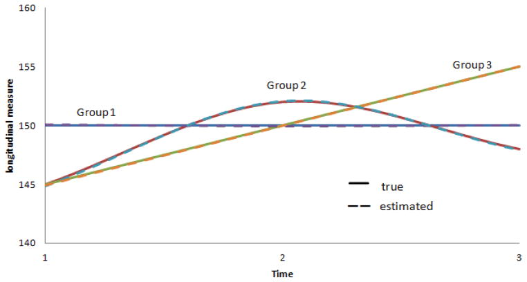
We simulated 500 datasets with a sample size of 150 to evaluate the discrimination index and the discriminatory ability of the models. We simulated datasets that consisted of a variety of trajectories and time points. We intentionally chose trajectories that intersect to induce ambiguity in the group memberships. One such combination of longitudinal trajectories is shown in Figure 1. Here we simulated three groups with roughly equal representation and overlapping trajectories using second degree polynomials. For simplicity, we did not add any time dependent or time independent covariates to the model.

Figure 1.

Three Group Trajectories

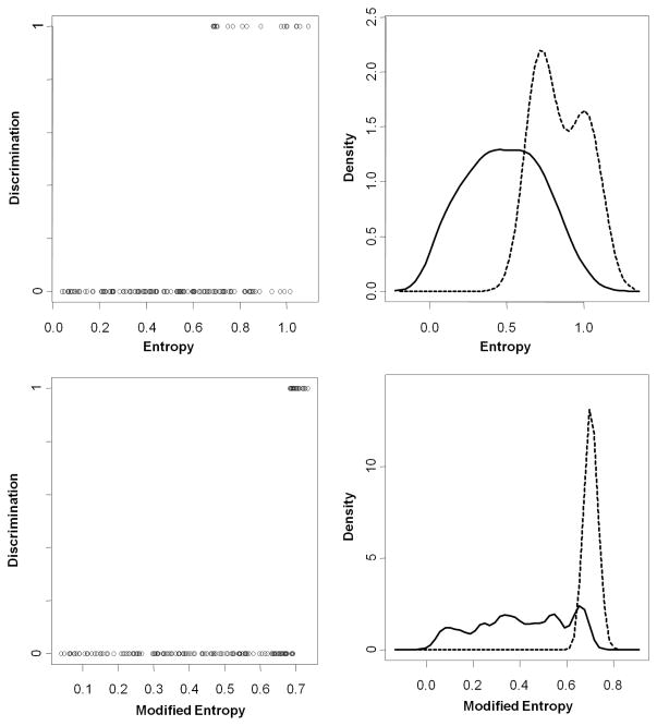
Table 1 summarizes the data generated according to simulated parameters along with the estimates. β_pj represents the p^th order polynomial for group j. The results in Table 1 show that the estimated parameters are close to the generated parameters. The three-group trajectory model also estimated the trajectories close to the underlying setting, as shown in Figure 1. The two group and four group models were also fit, and evaluation of the BIC showed that indeed the three group model is optimal. We then calculated, for each of the 500 datasets, how many subjects were poorly discriminated. Overall, the datasets averaged 19.47 poorly discriminated subjects per dataset, translating to a poor discrimination rate of 12.98%. Figure 2 depicts the density plots of entropy by the discrimination status for one such dataset. As expected, well discriminated subjects had a wide range of entropy, while poorly discriminated subjects tended to be at the upper end of the scale. Entropy ranged from 0.041 to 1.016 for the well discriminated subjects and from 0.685 to 1.094 for the poorly discriminated subjects. The overlap between discrimination and entropy takes place mainly when the posterior probability for one group is very low and nearly split between the two remaining groups. Since entropy is a measure of information, the measure provides information indicating that a subject most likely did not belong to the group with very low posterior probability. However, it has no way of discriminating between the other two groups. Two examples of this are shown in Table 2.

Table 1.

Three group simulation

parameter	simulated value	estimated values
θ1	0	−0.01
θ2	0	−0.01
β01	150	150.08
β11	0	−0.24
β21	0	0.11
β02	145	144.89
β12	12.50	12.80
β22	−5.50	−5.64
β03	145	144.91
β13	5	5.08
β23	0	−0.01
Σ	8	7.68

Figure 2.

Three group entropy and modified entropy. The dashed line represents poorly discriminated subjects, and the solid line represents acceptably discriminated subjects.

Table 2.

Entropy and discrimination for two simulated subjects. This shows how entropy and discrimination can differ.

ID	p̂1	p̂2	p̂3	Poor discrimination (0=no, 1=yes)	Entropy
115	0.26	0.21	0.53	0	1.02
145	0.01	0.47	0.52	1	0.75

The four group simulation, displayed in Figure 3, again showed that the estimated parameters and trajectories were very similar to the simulated parameters and trajectories. Applying the discrimination index, we found that, on average, 10.2% of the subjects were poorly discriminated.

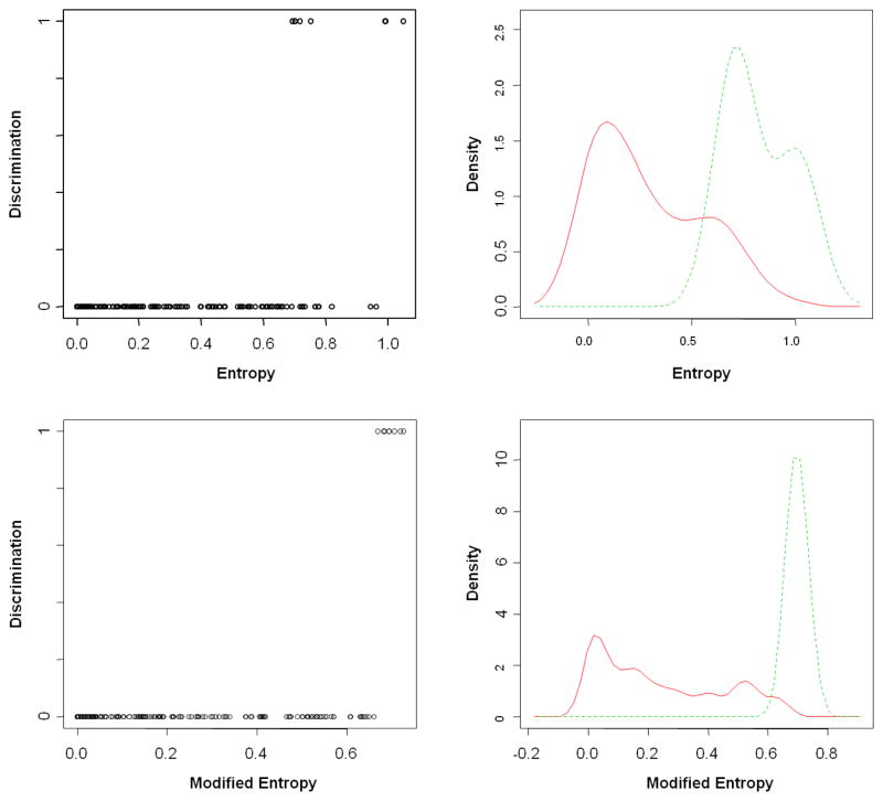
Figure 3.

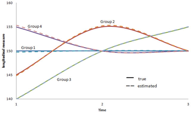
Four Group Trajectories

Figure 4 shows how entropy differs by discrimination status for one particular four group data set. It is evident that subjects who are poorly discriminated have higher levels of entropy than the well discriminated subjects, even though there is some overlap. Figure 2 also shows the distributions of entropy, with the solid line representing the density for well discriminated subjects and the dashed line for poorly discriminated subjects. As expected, our modified entropy measure performs better; there is more agreement between discrimination status and modified entropy.

Figure 4.

Four group entropy and modified entropy. The dashed line represents poorly discriminated subjects, and the solid line represents acceptably discriminated subjects.

Further simulations showed that adding more time points decreased the overall poor discrimination rate, and increasing the variance increased the overall discrimination rate. The three and four group models generated above, when extended to five longitudinal time points, yielded poor discrimination rates of less than 1%.

5. Example: The Pittsburgh Girls Study

The Pittsburgh Girls Study (PGS)[6] is a longitudinal study to follow an urban population sample of girls in Pittsburgh, Pennsylvania. The first assessment wave consisted of girls 5–8 years old. One objective of the study was to test developmental models for conduct disorder (CD). We fit latent group-based trajectory models to uncover distinct longitudinal trajectories of CD severity scores and then applied the discrimination index to show how many subjects are well and poorly discriminated into these groups. There were separate cohorts depending on the starting age of the child. We examined the cohort that entered as five year olds. The CD severity scores were based on the yearly self-reported information. Higher scores indicate more severe conduct problems while lower scores indicate fewer problems.

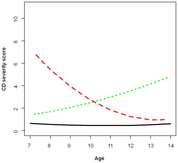
The cohort consists of 588 subjects followed yearly from age 5–14. We analyzed self reported data, which were collected from age 7 onwards. Only complete data cases were used, which reduced the dataset to N=471. There was no obvious pattern to the missing observations, and therefore they were assumed to be missing completely at random. We fit a latent-class longitudinal trajectory model with three groups, which is depicted in Figure 5. For simplicity, we did not include any covariates in the model. The number of groups was chosen based on BIC and clinical input to maintain a manageable number of groups.

Figure 5.

Trajectory plot for The Pittsburgh Girls Study. Group membership and descriptions can be seen in Table 3.

Table 4 shows the model results for the Pittsburgh Girls Study data. The trajectories showed one group (solid, 90%) that made up the majority of the cohort. These girls had a consistently low CD score over time. The group most interesting to researchers was denoted by the dotted line, and they made up 6.4% of the cohort. This is the group of girls whose conduct worsened over time. This group consists of girls whose conduct worsens as they age, and may be a signal to researchers that this group requires early behavioral intervention. It may also allow researchers to focus their efforts on studying this particular group to discover why they are getting worse over time. The results showed overlaps in the trajectories, which may indicate a high level uncertainty in group assignments. However, application of the discriminant index showed that only 5 of the 471 (1.1%) subjects were poorly discriminated. Overall, the subjects were very well discriminated into their groups. This may be due to the fact that one group contained a large proportion of the subjects. As Table 5 shows, poor discrimination rates were higher in the green group. Identifying these poorly discriminated subjects allows the investigators to examine them individually. Modified entropy also behaved as expected, with poorly discriminated subjects having higher modified entropy than acceptably discriminated subjects.

Table 4.

Pittsburgh Girls Study parameter estimates

parameter	estimated values
θ1	−2.64
θ2	−3.08
β01	0.65
β11	−0.11
β21	0.01
β02	1.39
β12	0.28
β22	0.03
β03	7.28
β13	−1.97
β23	0.15
Σ	1.89

Table 5.

Pittsburgh Girls Study results. The table shows group membership, percentage of poor discrimination, and the range of modified entropy.

Group	(n, %)	Poorly discriminated (n, %) within the group	Range of modified entropy among those not poorly discriminated	Range of modified entropy among those poorly discriminated
Solid	(423, 89.9%)	(3, 0.7%)	0.00–0.61	0.68–0.69
Dotted	(29, 6.1%)	(2, 6.7%)	0.00–0.55	0.66–0.67
Dashed	(19, 4.0%)	(0, 0.0%)	0.00–0.55	NA

6. Conclusions

The discrimination index and modified entropy are useful tools for evaluating latent group-based trajectory models. The discrimination index based on the delta methods can successfully identify subjects whose discrimination is too poor to confidently be assigned to a particular latent group. While entropy or modified entropy can help us measure the amount of uncertainty in discrimination, this index can place confidence intervals and help us develop cut-off rules in order to identify which subjects are poorly discriminated. The index provides a quick and effective way to analyze the results of a latent class or group-based model and identify individuals who may not truly belong to their assigned group. This can be very important, especially if interventions differ by group assignment. The index serves two purposes: first, to determine which individuals are poorly discriminated into their groups, and second, as a general test to evaluate the latent group-based trajectory model. Applying the method to The Pittsburgh Girls study showed that overall, the level of discrimination is very good. The discrimination index also identified which subjects were poorly discriminated during group assignment. The discriminant index provides a formal statistical test to determine an individual’s group membership status, and should be used in tandem with goodness-of-fit methods to evaluate latent group-based trajectory models. Future work could include performing a more thorough evaluation of different trajectories. One can simulate trajectories of various time points and parameters to identify conditions where group-based modeling discriminates well and poorly. Future work can also be done to evaluate the conditions under which these models are effective, including establishing guidelines for minimum longitudinal time points.

Table 3.

Four group simulation

parameter	simulated value	estimated values
θ1	0	−0.06
θ2	0	−0.01
θ3	0	−0.14
β01	150	148.75
β11	0	0.48
β21	0	−0.17
β02	145	144.87
β12	17.50	18.10
β22	−7.50	−7.76
β03	140	139.90
β13	12.50	12.60
β23	−2.50	−2.52
β04	155	155.32
β14	−7.50	−7.96
β24	2.50	2.63
Σ	8	7.53

References

- 1.Agresti A. Categorical Data Analysis. Wiley; New York: 1990. [Google Scholar]
- 2.Berkof J, Mechlen I, Gelman A. A Bayesian approach to the selection and testing of latent class models. Statistica Sinica. 2003;13:423–442. [Google Scholar]
- 3.Biernacki C, Govaert G. Choosing models in model-based clustering and discriminant analysis. Institut National de Recherche en Informatique et en Automatique. 1998;3509:1–22. [Google Scholar]
- 4.Collins L, Lanza S. Latent Class and Latent Transition Analysis. Wiley; New York: 2010. [Google Scholar]
- 5.Efron B. Bootstrap methods: Another look at the jackknife. The Annals of Statistics. 1979;7(1):1–26. [Google Scholar]
- 6.Keenan K, Hipwell A, Chung T, Stepp S, Stouthamer-Loeber M, Loeber R, Mc-Tigue K. The Pittsburgh Girls Study: Overview and initial findings. Journal of Clinical Child and Adolescent Psychology. 2010;39(4):506–521. doi: 10.1080/15374416.2010.486320. [DOI] [PMC free article] [PubMed] [Google Scholar]
- 7.Kreuter F, Muthen B. Analyzing criminal trajectory profiles: Bridging multilevel and group-based approaches using growth mixture modeling. Journal of Quantitative Criminology. 2008;24:1–31. [Google Scholar]
- 8.Lindsay B, Roeder K. Residual diagnostics for mixture models. Journal of the American Statistical Association. 1992;87(419):785–794. [Google Scholar]
- 9.Meneses J, Antle CE, Bartholomew MJ, Lengerich RL. A simple algorithm for delta method variances for multinomial posterior Bayes probability estimates. Communications in Statistics { Simulation and Computation. 1990;19(3):837–845. [Google Scholar]
- 10.Nagin DS. Group Based Modeling of Development. Harvard University Press; Cambridge, MA: 2005. [Google Scholar]
- 11.Nylund K, Asparouhov T, Muthen B. Deciding on the number of classes in latent class analysis and growth mixture modeling: A monte carlo simulation study. Structural Equation Modeling. 2007;14(4):535–569. [Google Scholar]
- 12.Titterington DM, Smith AFM, Makov UE. Statistical Analysis of Finite Mixture Distributions. Wiley; New York: 1985. [Google Scholar]