Learning From Data: Recognizing Glaucomatous Defect Patterns and Detecting Progression From Visual Field Measurements

Abstract

A hierarchical approach to learn from visual field data was adopted to identify glaucomatous visual field defect patterns and to detect glaucomatous progression. The analysis pipeline included three stages, namely, clustering, glaucoma boundary limit detection, and glaucoma progression detection testing. First, cross-sectional visual field tests collected from each subject were clustered using a mixture of Gaussians and model parameters were estimated using expectation maximization. The visual field clusters were further estimated to recognize glaucomatous visual field defect patterns by decomposing each cluster into several axes. The glaucoma visual field defect patterns along each axis then were identified. To derive a definition of progression, the longitudinal visual fields of stable glaucoma eyes on the abnormal cluster axes were projected and the slope was approximated using linear regression (LR) to determine the confidence limit of each axis. For glaucoma progression detection, the longitudinal visual fields of each eye on the abnormal cluster axes were projected and the slope was approximated by LR. Progression was assigned if the progression rate was greater than the boundary limit of the stable eyes; otherwise, stability was assumed. The proposed method was compared to a recently developed progression detection method and to clinically available glaucoma progression detection software. The clinical accuracy of the proposed pipeline was as good as or better than the currently available methods.

I. Introduction

Machine learning techniques have been widely used in biomedical applications [1]–[14]. Recent advances in data analysis and a significant growth in available database size have promoted classification methods that are capable of identifying previously hidden clusters and patterns in available datasets. In particular, unsupervised machine learning techniques can mathematically describe patterns in data without the use of prior class knowledge or heuristics [15]–[17]. Revealing these patterns can serve as a fundamental step toward more specific mining and learning tasks [18]. Such learning tasks recently have been applied to the detection and monitoring of glaucoma [9], [19]–[21].

Glaucoma is an optic neuropathy that is the second leading cause of blindness in the world [22]–[24]. Glaucoma management is dependent on identifying disease-related functional or structural defects and monitoring their progression over time. Recognition of glaucoma-related visual field defects (i.e., functional defects) is an aspect on which clinicians have relied since the mid-1800s [25]–[28]. For over a century, glaucoma specialists have accumulated knowledge to describe patterns of glaucoma-related visual field defects [29], [30]. Increased acceptance of Standard Automated Perimetry (SAP) testing about 25 years ago standardized visual field testing for glaucoma. Current SAP software includes a statistical analysis package and provides the clinician with information about visual function in the form of measurements of retinal sensitivity to light at 52 different test points (for 24-2 stimuli) across the central 24° of the visual field [25], [31]. Individual patient results also are compared to a normative database that provides the clinician an age-adjusted probability of abnormality for each test point.

A number of commercially available progression detection algorithms are included in the SAP software, such as progression by visual field index (VFI) [32] and guided progression analysis (GPA) [33]. These are statistical methods that use linear classification methods to represent the rate and magnitude of change (for VFI) or use variance analysis to identify change outside normal limits (for GPA), to classify eyes as progressing or stable. Recent advances in unsupervised classification techniques provide an alternative approach for glaucoma-related progression detection from SAP. For instance, machine learning and data mining techniques have been used to recognize glaucoma-related SAP visual field defect patterns and detect progression of glaucoma-related visual field defects [9], [19], [20], [34].

In the current study, we describe the performance of a Gaussian mixture model [35], [36] and expectation maximization (GEM) methods for 1) clustering eyes as glaucomatous or healthy and 2) discriminating between eyes with known glaucomatous progression and stable eyes. We compare the progression-detection performance of GEM to that of several other algorithms, including SAP software-based commercially available techniques (e.g., VFI and GPA). Results also are compared to those from a previously described unsupervised learning-based progression detection algorithm, progression of patterns (POP), which is based on change over time of patterns revealed using the variational Bayesian independent component analysis mixture model (VIM) [34], [37], [38]. We hypothesize that change in GEM-defined patterns of defect would perform as well as or better at detecting known glaucomatous change than other techniques. If our hypothesis is confirmed, change in GEM-defined patterns might be a better candidate for glaucoma progression detection from SAP data than change in VIM-defined patterns, because computational requirements to identify patterns are significantly less using GEM than VIM, and tracking change in VIM-defined patterns (i.e., POP) already has been shown to outperform some commercially available progression algorithms [19].

II. Methods

In this section, we first describe the instruments used to collect data, data acquisition, and the assessment of study participants. We then explain the mathematical derivations for modeling the data using GEM. We elaborate on the framework and implementation of the glaucoma progression-detection pipeline and the performance metrics employed. Next, we describe the clustering, boundary limit detection, and progression-detection testing steps. Finally, we report and discuss our results.

A. Instruments

Color photograph pairs were simultaneously obtained through maximally dilated pupils using a stereoscopic camera (Kowa nonmyd WX^3D, software version VK27E, Kowa Optimed Europe Ltd.). SAP-measured visual field sensitivity was tested at 52 points [54 points, with 2 blind-spot points excluded; see Fig. 1(b)] using the 24-2 SITA test strategy (Humphrey Field Analyzer II, Carl Zeiss Meditec Inc., Dublin, CA, USA). Fig. 1 (left) shows the optic disk region and peripapillary retina of a glaucomatous eye. Fig. 1 (right) displays the 24-2 SAP visual field measurements as absolute sensitivities in decibels at the available 52 test points that are uniquely specified by their angular location from fixation in the superior, inferior, nasal, or temporal zones.

Fig. 1.

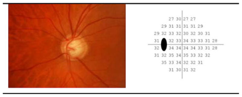
(Left) sample optic disk photograph image, (right) absolute sensitivities (in dB) of SAP visual points tested using the 24-2 system.

B. Data Acquisition and Assessment

All participant eyes were recruited from the University of California San Diego (UCSD)-based Diagnostic Innovations in Glaucoma Study (DIGS) and the African Descent and Glaucoma Evaluation Study (ADAGES) [39]. ADAGES is a multicenter study that includes UCSD, University of Alabama at Birmingham, and New York Eye and Ear Infirmary. Both studies follow the tenets of the Declaration of Helsinki, Health Insurance Portability and Accountability Act guidelines and the study site Human Research Protection Programs have approved all methodology. Written informed consent was obtained from all study participants.

Each study participant underwent a comprehensive ophthalmic evaluation, including review of medical history, best corrected visual acuity, slit-lamp biomicroscopy, intraocular pressure measurement with Goldmann applanation tonometry, gonioscopy, dilated slit-lamp fundus examination, simultaneous stereoscopic optic disk photography, and SAP visual field exam at each visit.

The current overall goals are to cluster glaucomatous visual fields into recognizable defect patterns, to establish a method of data representation, and to detect glaucomatous progression. Here, we explain how we created the reference standards for the clustering assessment and progression-detection steps. To create a gold standard for clustering assessment, all eyes were classified as abnormal (glaucomatous) or healthy based on the SAP software-provided glaucoma hemifield test (GHT) and pattern standard deviation (PSD). Eyes were considered abnormal if the instrument software defined GHT was outside of normal limits or if PSD ≤ 5% of normal, on two consecutive tests [40]. Healthy eyes had both GHT and PSD within normal limits. 939 eyes from 677 subjects were classified as abnormal and 1 146 eyes from 721 subjects were classified as healthy.

To create a reference standard for progression assessment, all eyes were classified as progressed or stable by evaluation of images of the optic disk. Optic disk images were chosen because they differed from the visual measurements being analyzed for progression. Hence, glaucomatous progression was based on structural evidence so as not to bias the detection of SAP-related visual field progression. Eyes showed progression or stability based on serial analysis of optic disk stereoscopic photographs. The baseline and each follow-up photograph were assessed for progressive glaucomatous optic neuropathy (PGON) by two expert-trained observers viewing digitized image pair on a 21-in or larger computer monitor. PGON was defined as a decrease in the neuroretinal rim width, or the appearance of a new or enlarged retinal nerve fiber layer defect in paired stereoscopic images. Observers were masked to the patient identification and diagnosis. A third observer adjudicated any disagreement in assessment between the first two observers [41]. 76 eyes from 70 subjects were identified as progressed by PGON (24 eyes also were labeled “likely progression” by SAP GPA). A total of 414 SAP visual field measurements were collected from this group. The mean number of follow-up visits was 5.5, and the mean follow-up time was 3 years.

Stable eyes were tested using SAP over a short period of time with the assumption that any change in measurements was due to variability in function of diseased ganglion cells or in attentiveness of the patient and not due to disease-related progression (this is because disease-related progression in adequately treated glaucoma eyes generally occurs over years, not weeks).

Stable glaucoma was simulated in a set of 91 eyes from 48 subjects that had been identified as glaucomatous at baseline with repeatable SAP defects, as defined earlier. Stable eyes were tested once a week, providing an average of 4.5 consecutive tests for each eye over an average of 4.3 weeks. A total of 428 SAP visual field measurements were collected from eyes in this group.

Table I shows the demographic information of the subjects in the abnormal and healthy visual field groups. Table II shows the demographic information of the subjects in the progressed and stable groups. The mean deviation (MD) and PSD of each group, global indices that indicate the deviation of a visual field from a mean of normal visual field, also are listed in both Tables.

TABLE I.

Demographic Information of Subjects Used for Clustering

Parameter	Abnormal Visual Field	Normal Visual Field	p-value
Number of eyes	939	1146	-
Number of subjects	677	721	-
Age at baseline in years (SD)	58.6 (14)	46.8 (14.5)	<0.01
Gender (percent female)	40	46	-
SAP Mean Deviation (MD) in dB (SD)	−4.3 (4.9)	−0.46 (1.3)	<0.01
SAP Pattern Standard Deviation (PSD) in dB (SD)	4.4 (3.2)	1.5 (0.24)	<0.01

TABLE II.

Demographic Information of Subjects and Follow-up Visits Used for Progression Detection

Parameter	Progressed based on photo	Stable	p-value
Number of eyes	76	91	-
Number of subjects	70	48	-
Number of Follow-ups (SD)	5.5 (4.2)	4.7 (0.80)	<0.01
Length of Follow-up (SD)	2.7 years (2.1)	4.2 weeks (1.4)	<0.01
Age at baseline in years (SD)	62.6 (12.6)	71.0 (9.5)	<0.01
Gender (percent female)	53	45	0.14
Baseline SAP Mean Defect (MD) in dB (SD)	−4.1 (4.8)	−7.4 (8.2)	<0.01
Baseline Pattern Standard Deviation (PSD) in dB (SD)	5.1 (4.2)	6 (4.2)	0.14

C. Data Modeling Using Gaussian Mixture Model-Expectation Maximization

Assume we have n samples of data and that each sample has d dimensions. The goal is to model the given data with a c-component Gaussian mixture model. Let Y = [Y₁, …, Y_d]^T represent the d-dimensional Gaussian random variable and let y = [y₁, …, y_d]^T represent a particular outcome of Y. Then, the probability distribution function of a c-component finite Gaussian mixture model can be written as [35], [36]

$$p(\mathit{y}\mid \theta )=\sum _{m=1}^c{\alpha }_{m}p(\mathit{y}\mid {\theta }_m)$$ (1)

where α₁, …, α_c are weights of each mixing distribution, and each θ_m is the set of parameters defining the mth mixing distribution component. Therefore, the complete set of model parameters can be written as {θ₁, …, θ_c, α₁, …, α_c}.

Assume the data samples, = {y⁽¹⁾, …, y⁽ⁿ⁾} are independent and identically distributed. Then, we can write the log-likelihood of the c-component Gaussian mixture model as

$$logp(\mathcal{Y}\mid \mathit{\theta })=log\prod _{i=1}^{n}p\left(y^{(i)}\mid {\theta }_m\right)=\sum _{i=1}^{n}log\sum _{m=1}^c{\alpha }_{m}p\left(y^{(i)}\mid {\theta }_m\right)$$ (2)

with constraints on the weighting coefficients as α_m ≥ 0, m = 1, …, c and ${\displaystyle \sum _{m=1}^c}{\alpha }_m=1$.

The main approaches below can be followed to find the parameters of this model. The maximum likelihood (ML) estimate can be written as

$${\widehat{\mathit{\theta }}}_{\text{ML}}=argmaxlogp(\mathcal{Y}\mid \mathit{\theta })$$ (3)

The maximum a Posteriori (MAP) criterion can be written as

$${\widehat{\mathit{\theta }}}_{\text{MAP}}=argmax\{logp(\mathcal{Y}\mid \mathit{\theta })+logp(\mathit{\theta })\}$$ (4)

where p(θ) is the prior on the parameters.

It is well known that neither ML nor MAP estimates can be found analytically. The expectation maximization (EM) is the proper choice for computing the parameters in ML or MAP. Using EM in an iterative procedure, the local maximum of ML or MAP can be found. Assume that = {z⁽¹⁾, …, z⁽ⁿ⁾} indicate which Gaussian mixture component produced each data sample. Therefore, each label is a binary vector ${\mathbf{z}}^{(i)}=\left[z_1^{(i)},\dots ,z_c^{(i)}\right]$, where $z_m^{(i)}=1$ and $z_q^{(i)}=0$ for q ≠ m, means that the sample y⁽ⁱ⁾ was generated by the mth Gaussian mixture component. Adding membership data to the model, we can write

$$logp(\mathcal{Y},\mathcal{Z}\mid \mathit{\theta })=\sum _{i=1}^n\sum _{m=1}^c{z}_m^{(i)}log[{\alpha }_{m}p(y^{(i)}\mid {\theta }_m)].$$ (5)

Then, the Expectation step can be written as [42]

$$Q\left(\theta ,\widehat{\mathit{\theta }}(t)\right)\equiv E[logp(\mathcal{Y},\mathcal{Z}\mid \mathit{\theta })\mid \mathcal{Y},\widehat{\mathit{\theta }}(t)]=\text{log}p(\mathcal{Y},\mathcal{W}\mid \mathit{\theta })$$ (6)

where = E[ | θ̂(t)] and {t = 0, 1, 2, …} represents a time sequence.

Because the elements of are binary, we can write

$$\begin{array}{l}{w}_m^{(i)}\equiv E[z_m^{(i)}\mid \mathcal{Y},\widehat{\theta }(t)]=Pr[Z_m^{(i)}=1\mid {\mathcal{Y}}^{(i)},\widehat{\theta }(t)]\\ =\frac{{\widehat{\alpha }}_m(t)p({\mathit{y}}^{(i)}\mid {\widehat{\theta }}_m(t))}{{\sum }_{j=1}^c{\widehat{\alpha }}_j(t)p({\mathit{y}}^{(i)}\mid {\widehat{\theta }}_j(t))}.\end{array}$$ (7)

In the case of MAP, the maximization step can be written as

$$\widehat{\mathit{\theta }}(t+1)=argmax\left\{Q\left(\mathit{\theta },\widehat{\mathit{\theta }}(t)\right)+logp(\theta )\right\}.$$ (8)

The EM algorithm is iterated until reaching a convergence criterion.

III. Glaucoma Progression Detection Pipeline

The pipeline used for glaucoma progression detection is composed of three stages: clustering, glaucoma boundary limit detection, and glaucoma progression detection testing (see Fig. 2). In Fig. 2, the clustering stage is shown at the top, the boundary limit detection in the middle, and the progression detection testing at the bottom. The axes, which make up the output of the top stage, are the input to the second stage. A different dataset was used to complete each stage. We used a dataset of abnormal and within normal limits (i.e., healthy) SAP visual fields (refer to Table I) for the clustering stage, a dataset of stable glaucoma visual fields (refer to Table II, column 2) for the boundary limit detection stage, and we used a dataset containing time sequences of SAP visual fields of PGON eyes (i.e., those designated as progressing by optic disc assessment) in the progression-detection testing stage (refer to Table II, column 3). We will explain each stage in more detail in the subsequent sections.

Fig. 2.

Glaucoma progression detection pipeline.

A. Implementation and Performance Metrics

The GEM data modeling introduced in the previous section essentially combined multivariate Gaussian components to model the visual field data points. Number of samples, n, was 2 085 and the number of dimensions, d, was 53 (52 SAP absolute sensitivity values and age). Clusters were assigned by selecting the component that maximized the MAP based on the EM-estimated parameters. Principal component analysis (PCA) was utilized to decompose each cluster into several axes. To identify a globally optimal GEM model that represents glaucoma category and visual field defect patterns, we generated several GEM models and selected a model that provided the best sensitivity at near 95% specificity. We chose the number of clusters in our GEM models, c, as three to reflect the three broad categories of visual field namely, normal, early, and advanced glaucoma. All stages of the model were implemented in MATLAB (Mathworks, Natick, MA, USA). The following performance metrics were utilized to assess the accuracy of the clustering stage.

1) True Positives (TP), which are positive instances correctly classified as positive, 2) False Positives (FP), which are negative instances incorrectly classified as positive, 3) True Negatives (TN), which are negative instances correctly classified as negatives, and 4) False Negatives (FN), which are positive instances incorrectly classified as negatives.

Specificity is defined as the proportion of all those without disease correctly identified as negative.

$$\text{Specificity}=\frac{\text{TN}}{\text{TN}+\text{FP}}.$$

Sensitivity is defined as the proportion of all those with diseases correctly identified as positive.

$$\text{Sensitivity}=\frac{\text{TP}}{\text{TP}+\text{FN}}.$$

We assessed the performance of the clustering stage using the reference standard dataset (abnormal and normal SAP visual fields) and the sensitivity/specificity performance metrics defined previously. To assess the relative performance of the entire pipeline, we compared the outcome of our method to GPA [33], linear regression (LR) of the VFI, and LR of the MD. GPA indicates visual field change from baseline by evaluating all test points and indicates “likely progression” for the full field if visual field change (greater than the variability observed in two baseline measurements) in three or more of the same points is repeatable in three consecutive exams [33]. The VFI and MD are global indices provided for each individual test. We also compared the performance of GEM with that of the previously described VIM-based method [19]. We will provide the details of the assessments in the subsequent sections.

B. Clustering Stage

The absolute visual field sensitivity values from the 52 perimetric locations (54, excluding 2 blind spot locations) and age were used as input to GEM for data modeling. Age was included because both glaucomatous and normal visual fields expressed as absolute sensitivity are affected by age, and age was used in the previous unsupervised learning studies [10], [34], [43]. The unsupervised clustering was performed using the GEM model to detect glaucomatous visual field defects. Using the 2 085 SAP visual fields (cross sectional) as input, GEM modeled c categories of glaucoma stages (i.e., c clusters) from the data and assigned each of these visual fields to the best fitting cluster. The initiating variable for the learning process was the number of mixing Gaussians, their mean and variance, and the number of clusters, c, which ranged from c = 2–5. Validation was done after learning the clusters by observing the distribution of abnormal and normal fields in each cluster and the GEM model with nearly 95% specificity and the highest sensitivity was selected from 600 trained GEM models. Fig. 3 shows the specificity versus sensitivity for 600 trained GEM models.

Fig. 3.

Performance of all trained GEM models.

From our assessment of sensitivity-specificity tradeoff among the 600 training GEM models, we found that three clusters provided a better separation of glaucoma and healthy fields. These three clusters were categorized into normal cluster N, moderate glaucoma cluster G1, and advanced glaucoma cluster G2 depending on the centroid of the raw threshold sensitivities of these clusters (normal fields have higher threshold values than glaucomatous fields). In Fig. 4, we show 2-D scatterplots of these 53-D clusters for visualization. Fig. 4 (top) shows the scatter plot of the superior hemifield (i.e., all visual field locations above the middle horizontal meridian shown in Fig. 1) average threshold versus the inferior hemifield (all visual field locations below the middle horizontal line as in Fig. 1) average threshold for all eyes.

Fig. 4.

2-D Scatter plot of features. (Top) average of superior hemifield versus average of inferior hemifield. (Bottom) MD versus PSD.

As can be seen from this figure, the eyes in different clusters are organized from top right to the bottom left. The clinical interpretation of this organization is discussed in Results and Discussion section. Fig. 4 (bottom) shows the scatter plot of MD versus PSD (two global clinical indices of visual function) for all eyes. As can be seen from this figure, three clusters have been organized from high to low MD and PSD values.

We decomposed all of the visual fields comprising each cluster into different axes using PCA. The visual fields associated with each axis define the patterns of visual defect that we are seeking. Within each cluster, the relative contribution of each axis was assessed based on its respective eigenvalue. Only axes with significant contributions (high eigenvalues) were retained in a cluster. The number of axes in clusters N and G₁ was 2 each, and the number of axes in cluster G₂ was 5.

To organize the visual field loss patterns from mild to advanced, the visual field patterns are represented as axes through each cluster centroid. Clinicians typically rely on the total deviation (TD) or pattern deviation (PD) plots supplied by the HFA Statpac analysis (Carl Zeiss Meditec, Inc., Dublin, CA, USA). We used simulated TD plots in our analysis to display the patterns of visual defects in relation to normal eyes. The simulated TD plot is a 52-D vector obtained by subtracting absolute sensitivities at the centroid of the normal cluster N from the absolute sensitivities at the centroid of the glaucomatous clusters, and then, representing field defects as plots at −2, 0 (cluster centroid), and +2 standard deviation (SD) along each of the axes. The numerical TD-like plots were further converted into color representations to aid in visualization. The −26 to +26 values were displayed in equal steps of color from red to green, with −26 as pure red and +26 as pure green.

Fig. 5 (first row) shows the generated mean patterns of each cluster after TD simulation.

Fig. 5.

VF patterns represented by the centroid of each GEM cluster. Increased red saturation indicates increased deterioration of the visual field. The top left pattern represents the visual fields the cluster N, the top middle showing early visual field deterioration represents cluster G₁, and the top right showing mild to advanced visual field deterioration represents cluster G₂. The bottom figure is the color-coding legend.

The centroid of the first cluster (see Fig. 5 left) has zero dB MD at all points and is composed mostly of normal visual fields (cluster N), the centroid of the second cluster (see Fig. 5 middle) deviates −2.6 dB on average from the normal mean and is composed mostly of abnormal visual fields (cluster G₁), and the centroid of the third cluster deviates −9 dB on average from the normal mean (see Fig. 5 right) and is composed only of abnormal visual fields (cluster G₂). The color coded legend used to display the TD simulated plot patterns is shown in Fig. 5 (second row).

We created the patterns along each axis by adding to or subtracting from the cluster centroid, 2 standard deviations along that axis direction (i.e., ± 2 SD). Fig. 6 shows the visual field patterns at +/−2 SD along each cluster axis within each cluster. Using the distance between each 52-D visual field and each of the axes within each of the three clusters, we assigned each visual field to its closest axis within the closest cluster.

Fig. 6.

VF patterns (axes and +/−2SD) in three clusters N, G1, and G2 generated by GEM. The representation simulates total deviation plots generated at −2/+2 standard deviation units on each axis. Increased red saturation indicates increased deterioration of the visual field.

For further examination, the visual fields were projected on to their respective assigned axes and the visual fields assigned to each axis were sorted depending on their projection magnitudes from the cluster centroid.

Sorting the visual fields from negative to positive depicts the earliest visual field defects to the most advanced ones. The visual fields were noted for their resemblance to the generated fields on the axis, to the similarity of other visual fields assigned to the same axis, and for the consistency in increasing severity as the visual fields were located further in the positive direction along the axis. This procedure will be discussed in Section IV.

C. Glaucoma Boundary Limit Detection Stage

We performed glaucoma boundary limit detection by projecting the longitudinal sequence of visual fields of each stable eye in the 53-D space onto each of the seven predefined GEM glaucoma axes as identified by the clustering stage (refer to Section II-B and Table II to recall stable group definition and demographic information). We then permuted the visual field sequence of each stable eye to maximize the number of slopes used to determine the percentile limit (PL) for stable eyes on each axis. For an eye with five consecutive visits, we generated 5!(= 120) longitudinal sequences of VFs, and then, we projected each sequence on the axis. The temporal interval between visits for each stable eye was about one week; however, we reset this interval to one year to approximate the limits of stability of eyes and to be in agreement with the convention that glaucoma patients are commonly followed at intervals between six months to one year. Next, we approximated the slope of each longitudinal series of projected visual fields by a LR. Due to the intervisit variability of the visual fields, the longitudinal sequence of visual fields from some stable eyes have a positive slope, indicating improvement, while others have a negative slope, suggesting deterioration.

The 95th single tail percentiles toward the direction of deterioration for all seven axes for detecting glaucoma progression were then calculated. Single tail was used, because we were interested only in significant deterioration and were not interested in significant improvement. Because eyes in the stable group presumably showed no disease related progression, the variability in this group was used to define the maximum variability that indicated no change. Fig. 7 demonstrates the histograms of all the approximated slopes after projecting the longitudinal visual fields of the stable eyes on each axis of clusters G₁ and G₂.

Fig. 7.

Histogram of the projected slopes. Top row shows the histogram of the slopes after projecting the stable group’s longitudinal visual fields on axis 1 and 2 of the cluster G₁, middle row represents the histogram of the slopes after projecting the stable group’s longitudinal visual fields on axis 1, 2, and 3 of cluster G₂, and bottom row shows the histogram of the slopes after projecting the stable group’s longitudinal visual fields on axis 4 and 5 of cluster G₂.

Table III lists the 95th PL for glaucoma progression detection after projecting the longitudinal visual field of stable eyes on axes of clusters G₁ and G₂ (identified at the clustering stage), and then, approximating the slopes by an LR model. The 95th PL of the empirical histogram of the slopes for each axis alone indicates that if we project the visual field of an eye and it falls above this limit, the eye is stable, otherwise, the eye is classified as progressed at 5% level of significance.

TABLE III.

95% Percentile Limit of Stable Eyes for Each Axis

Cluster Axis	G1 axis 1	G1 axis 2	G2 axis 1	G2 axis 2	G2 axis 3	G2 axis 4	G2 axis 5
95th PL limit	−0.70	−0.20	−0.70	−0.35	−0.40	−0.35	−0.30

D. Glaucoma Progression Detection Testing Stage

For progression detection, we projected the longitudinal series of visual fields on to each glaucoma axis (axes determined at the clustering stage), and then, we approximated the average progression rate (slope) of each sequence along the glaucoma axes using an LR model. For each eye, if the approximated slope passes the 95% PL of that axis (the line falls below the stable cutoff limit), the eye was classified as progressed; otherwise, the eye was classified as stable. The progression detection stage essentially uses GEM to detect POP during glaucoma progression, therefore, we call the entire pipeline GEM-POP. We have shown the outcome of the proposed GEM-POP for four example eyes in Fig. 8. The eye in Fig. 8 (top left) provided ten visual field tests collected from 2000 to 2006, the eye in Fig. 8 (top right) provided seven visual field tests collected from 2003 to 2007, the eye in Fig. 8 (bottom left) provided 11 visual field tests collected from 2000 to 2007, and the eye in Fig. 8 (bottom right) provided ten visual field tests collected from 2001 to 2007. The orange circles indicate the severity after projecting the 53-D data onto the first axis of cluster G₂. The blues circles indicate the estimated mean slope of projected values by LR (through the orange circles). Note that the y-intercept of all severity lines is zero for these comparisons. We also adjusted the curve of actual projected values accordingly, to start from zero severity at baseline. The gray line indicates the 95% PL for the slopes of the first axis of cluster G₂. This cutoff limit was determined using the percentile boundary limit detection stage utilizing the stable eyes described in the previous step. If the linear model approximating the slope fell below the gray line (progression zone), then the eye was classified as progressed, otherwise, the eye was classified as stable. Therefore, the eyes in Fig. 8 (top row) are classified as progressed, because the blue line for both falls in the progression zone and the eyes in Fig. 8 (bottom row) are classified as stable, because the blue line for both falls in the stable zone.

Fig. 8.

gray line indicates the 95th percentile limit for progression rate, the orange circles represent the actual projected visual field values on the first axis of cluster G₂, and the blue circles are the linear regressed line approximating the projected visual field values on the first axis of cluster G₂.

Even though the slope of the blue line that indicates the change in severity of glaucoma is negative (suggests deterioration) in the two eyes displayed at the bottom Fig. 8, the change is not significantly negative; hence, the eyes are classified as stable. This indicates that the rate of deterioration is the factor indicative of progression. For assessing the GEM-POP performance, we used longitudinal SAP visual fields from eyes with known progressing glaucoma, which will be discussed in more detail in the next section.

IV. Results and Discussion

We selected the best model out of 600 models, generated by the clustering stage, which contained three clusters. The MD value (global index of deviation from normal visual field) of each cluster approximates the clinical assessment of disease severity. Cluster N was mostly composed of normal visual fields with an average mean defect (MD) of −0.53 ± 1.3 SD, Cluster G₁ was mostly composed of early glaucoma visual fields with an average MD of −2.3 ± 1.6 SD and Cluster G₂ was composed of mild to advanced glaucoma visual fields with an average MD of −8.7 ± 6.4 SD.

Cluster N was composed of 1 237 visual fields (1102 normal and 135 abnormal fields), Cluster G₁ was composed of 530 visual fields (44 normal and 486 abnormal), and Cluster G₂ was composed of 318 visual fields (0 normal and 318 abnormal). The specificity was 96% for placing normal fields in Cluster N, and the sensitivity was 87% for placing abnormal visual fields in either Cluster G₁ or G₂. Because the structures of Cluster N and Cluster G₁ were represented by two axes, and the structure of Cluster G₂ was represented by five axes, all visual fields patterns were characterized by a total of nine principal axes.

We characterized the patterns at points on an axis on the positive and negative sides (± 2 SD) of the cluster mean, generating 18 patterns.

Most of the normal fields were represented by two axes in Cluster N, and most of the glaucomatous fields were represented by seven axes in Clusters G₁ and G₂; resulting in 14 patterns of abnormal visual fields. As can be seen in Fig. 5 (left), the simulated TD plot for the first cluster’s (N) centroid resulted in 0 dB at all test locations, and the generated fields at −2 and +2 SD on axis 1 (see Fig. 6, first and second rows) were uniformly mildly depressed (−2 dB) or above normal (+2 dB), respectively. The generated fields at −2 SD and +2 SD of axis 2 were within ±1 dB at each hemifield. The simulated TD plot for the second cluster’s (G₁) centroid (From Fig. 5 middle) resulted in average −2.6 dB, and the generated fields at all locations on both axes were between 0 and −7 dB (see Fig. 6, third and fourth rows). From Fig. 5 (right), the simulated TD plot for the third cluster’s (G₂) centroid resulted in about −9 dB, and the generated fields at all locations on all five axes were between −1 and −22 dB (see Fig. 6, fifth and sixth rows).

The clustering stage assigned most of the normal eyes to axes 1 and 2 of cluster N based on the minimum distance of the visual field from each axis. From the total eyes in the normal cluster, 849 eyes were assigned to the first axis and 139 eyes were assigned to the second axis of the normal cluster. From the total eyes in cluster G₁, 76 eyes were assigned to the first axis and 31 eyes were assigned to the second axis. From the total eyes in cluster G₂, 158 eyes were assigned to the first axis, 5 eyes to the second axis, 44 eyes to the third axis, 41 eyes to the fourth axis, and 40 eyes were assigned to the fifth axis.

In addition to the fact that age is a significant risk factor for glaucoma, baseline age in this study was also significantly different between normal and abnormal eyes (p < 0.01; Table I). There is a possibility that age might affect the clustering outcome significantly. To evaluate the effects of age on the clustering outcome, we also assessed the performance of the clustering step excluding age. The best clustering model without age was 96% specific and 86.4% sensitive (versus 96% and 87% with age, respectively). Therefore, it is evident that the clustering outcome is not significantly affected by age. From machine learning perspective, this indicates that the spatial VF data without age information contains sufficient diagnostic information to maintain a high discriminative/diagnostic power.

To examine the individual visual fields associated with each axis, we projected the visual fields associated with an axis and sorted them by their projection on (i.e., distance along) that axis. The sorted visual fields from negative to positive indicated the earliest field defects to most advanced field defects. Fig. 9 shows the visual field patterns of sample eyes along the first axis of each cluster. Fields are shown as absolute sensitivities (top) and simulated TD plots (bottom) from three sample eyes (from left to right) from the first axis of each cluster. Note that the GEM clustering stage generates seven glaucoma axes, as explained earlier. If we define progression detection based on any one axis that indicates progression, GEM-POP has seven chances to detect progression; in contrast, GPA, MD, and VFI each have only one chance to detect progression.

Fig. 9.

VF absolute sensitivity values and TD simulated patterns for three eyes in abnormal clusters assigned to the first axis of that cluster. Projecting the VF of each eye on the first axis, and then, sorting the values from the most negative to the most positive, calculated the severity. The VF thresholds and TD simulated values for eyes corresponding to the most negative, mid, and most positive projected severities are placed from left to right, respectively.

To compensate for this advantage for GEM-POP, we adjusted the specificity of each axis upwards to achieve an overall specificity of 95%. This compensation resulted in larger cutoff values for stability for the individual axes than those listed in Table III. We minimized the effect of differences among the algorithms by equating for specificity prior to determining progression. Table IV lists the adjusted 95th PL for each axis to reach overall 95% specificity on stable eyes.

TABLE IV.

95th Percentile Limit of Stable Eyes to Reach Overall 95% Specificity on all Axes

Cluster Axis	G1 axis 1	G1 axis 2	G2 axis 1	G2 axis 2	G2 axis 3	G2 axis 4	G2 axis 5
95th PL limit	−1.00	−0.65	−1.00	−0.50	−0.65	−0.65	−0.65

To test the performance of our proposed framework, we analyzed 76 progressed eyes (refer to the progressed column of Table II). We projected the longitudinal SAP visual fields of all eyes on all seven axes of clusters G₁ and G₂, and we then, computed the approximated slopes by LR for each axis. Then, for each eye, we compared the slope of the linear fit to the 95th percentile limit for stable eyes (refer to Table IV) on each axis. If at least one of the axes showed progression, we classified the eye as progressed; otherwise, we classified the eye as stable. To further analyze the effectiveness of GEM-POP, we compared its performance for identifying known progressing eyes to LR of three available visual field diagnostic indices, MD, and VFI. Table V lists the progression detection outcomes of GEM-POP, GPA, MD, and PSD.

TABLE V.

Progression Detection Performance Comparison

Progression detection method	Percent of eyes identified as progressed	p-value compared to GEM_POP
GEM-POP	28.9%	-
GPA	19.7%	0.05
MD	16.9%	0.02
VFI	14.1%	<0.01

Similar to GEM-POP, we defined the 95th percentile limits of stability based on the permutation distribution of the stable eyes and defined progression by MD and VF.

We also compared the GEM-POP outcome to the recently developed VIM progression of patterns (VIM-POP) method [19], for the same eyes and for the same follow-up duration, and found that GEM-POP performed slightly but not significantly better than VIM-POP (sensitivity for VIM-POP was 26.6% compared to 28.9% for GEM-POP).

The percentage of correctly identified known progressing eyes (sensitivity) is somewhat low for all methods. There are several explanations for this finding. First, structural change (used as the reference standard for progression in this study) and functional change (based on SAP) do not necessarily occur at the same time [44]. Second, it is often difficult to detect actual change in VFs from noise due measurement error and random variation. This can be alleviated partly by modeling spatial correlation within visual fields, while considering the relationship between the spatial arrangements of the visual fields and the anatomy of the eye. We have not considered spatial dependence in this paper; however, it could be investigated in future work. Third, progression detection may be less than ideal due to the lack of a ground truth reference standard.

In GEM-POP, the clustering stage uses a mixture of Gaussians to model the data, to identify the clusters and to decompose each cluster to several axes based on PCA. In VIM-POP, cluster identification and ICA axis decomposition is performed within a single step, making implementation very complex and creating a computationally complex model. Creating a progression detection environment using GEM-POP takes minutes on a standard PC, while creating such an environment using VIM-POP takes several days. It is worth mentioning that GPA and LR of MD and VFI all use linear statistical methods to detect progression that lack the inherent benefits of machine learning-based methods.

In addition, we have shown that the clustering stage capable of effectively extracting useful features from high-dimension data space (e.g., pointwise visual thresholds) can improve the sensitivity of detecting progression compared to selective 1-D global indices such as MD and VFI. In contrast to global indices, GPA uses high-dimensional data for analysis. Therefore, the comparison of GEM-POP with GPA further emphasizes the strengths of GEM-POP including its strengths of extracting useful features in the clustering stage.

The future direction of this study can be devoted to assessing the glaucoma progression detection rate using other ophthalmic data.

V. Conclusion

A pipeline for recognizing glaucomatous visual field defect patterns and identifying glaucomatous progression was demonstrated. The visual field data were modeled using a mixture of Gaussians and the model parameters were estimated using expectation maximization. Then, the visual field data were clustered successfully into one normal and two glaucoma clusters (each representing disease severities). The relatively good performance of our clustering stage confirms its relative effectiveness in structuring data. Each cluster was decomposed to several axes using PCA to identify glaucomatous progression. Glaucoma cutoff limits were calculated on all identified glaucoma axes and were used to detect progression. A dataset of progressing glaucomatous eyes was used to assess the performance of the entire glaucoma progression pipeline and the outcome of our method was compared to commercially available glaucoma progression detection software algorithms and a recently published algorithm for progression detection. Overall, progression detection based on the Gaussian mixture model using expectation maximization identified significantly more known progressing eyes than all but one commercially available SAP progression detection method. Progression detection based on change in GEM-POP defined axes performed slightly better than progression detection using VIM-POP, while being far less computationally complex. The run time for clustering and axis identification using GEM-POP is a small fraction of the run time required to perform the same tasks using the methodology on which VIM-POP is based.

Biographies

Siamak Yousefi (S’09–M’12) received the Ph.D. degree from the University of Texas at Dallas, Richardson, TX, USA.

He is currently a Postdoctoral Fellow at the Hamilton Glaucoma Center, University of California at San Diego, CA, USA, where he is conducting research on ophthalmic image and data analysis. His research interests include biomedical image analysis, pattern recognition, and machine learning.

Dr. Yousefi is a member of the ARVO.

Michael H. Goldbaum received the M.D. degree from Tulane University, New Orleans, LA, USA (MD) and the M.S. degree in medical informatics from Stanford University Stanford, CA, USA.

He is an Ophthalmic Surgeon, an Educator, and a Scientist and is a Professor of ophthalmology at the University of California at San Diego, CA, USA. He is the Director of Glaucoma Informatics Research, where he applies medical image analysis and machine learning classifiers to improve care of eye diseases.

Madhusudhanan Balasubramanian received the Ph.D. degree from Louisiana State University, Baton Rouge, LA, USA.

He is currently an Assistant Professor in the Department of Electrical and Computer Engineering at the University of Memphis, Memphis, TN, USA. His research interests include the intersection of computational science and engineering, biosolid mechanics and biofluid dynamics with emphasis in studying ocular structures, and dynamics and the mechanism of vision loss in glaucoma.

Felipe A. Medeiros received the graduate degree and residency from the University of Sao Paulo.

He is a Professor of ophthalmology and the Medical Director of the Hamilton Glaucoma Center, University of California San Diego, CA, USA. He is also the Director of Vision Function Research at the same institution.

Linda M. Zangwill received the M.S. degree from the Harvard School of Public Health and the Ph.D. degree from Ben-Gurion University of the Negev.

She is a Professor of ophthalmology at the University of California, San Diego, CA, USA. His research interests include improving our understanding of the complex relationship between structural and functional changes in the aging and glaucoma eye, and developing computational techniques to improve glaucomatous change detection.

Jeffrey M. Liebmann completed his ophthalmology residency at the State University of New York/Downstate Medical Center and his fellowship in glaucoma at the New York Eye and Ear Infirmary of Mount Sinai.

He is presently a Clinical Professor of ophthalmology at New York University School of Medicine, New York, NY, USA and the Director of Glaucoma Services at Manhattan Eye, Ear, and Throat Hospital, New York and New York University Langone Medical Center, New York and an Adjunct Professor of clinical ophthalmology at New York Medical College, Valhalla, NY.

Christopher A. Girkin is the Chairman of the Department of Ophthalmology and a Chief Medical Officer for the Callahan Eye Hospital, the University of Alabama at Birmingham (UAB), AL, USA. After residency at the UAB, he completed a fellowship in neuro-ophthalmology at the Wilmer Eye Institute at Johns Hopkins, Baltimore, MD, USA and in Glaucoma at the Hamilton Glaucoma Center, the University of California, San Diego, CA, USA.

Robert N. Weinreb received the electrical engineering degree from the Massachusetts Institute of Technology, Cambridge, MA, USA and the M.D. degree from Harvard Medical School, Boston, MA.

He is a Clinician, a Surgeon, an Educator, and a Scientist. He is the Distinguished Professor of ophthalmology and the Chairman of the Department of Ophthalmology at the University of California, San Diego, CA, USA.

Christopher Bowd received the Ph.D. degree from Washington State University, Pullman, WA, USA.

He is currently a Research Scientist at the Hamilton Glaucoma Center, University of California, San Diego, CA, USA. His current work involves early detection and monitoring of glaucoma with structural imaging of the optic nerve, visual function and electrophysiological testing using standard and machine learning classifier-based analyses.

References

- 1.Yousefi S, Kehtarnavaz N, Akins M, Luby-Phelps K, Mahendroo M. Separation of preterm infection model from normal pregnancy in mice using texture analysis of second harmonic generation images. Proc IEEE Eng Med Biol Soc Conf. 2010;2010:5314–5317. doi: 10.1109/IEMBS.2010.5626349. [DOI] [PubMed] [Google Scholar]
- 2.Yousefi S, Kehtarnavaz N, Akins M, Luby-Phelps K, Mahendroo M. Distinguishing different stages of mouse pregnancy using second harmonic generation images. Proc. 42nd Southeastern Symp. Syst. Theory; 2010; pp. 44–46. [Google Scholar]
- 3.Yousefi S, Kim B, Kehtarnavaz N. Automating porosity features extraction from second harmonic generation images of cervical tissue. Proc. IASTED Int. Conf. Signal Image Process.; 2011; pp. 129–132. [Google Scholar]
- 4.Ohno-Machado L. Research on machine learning issues in biomedical informatics modeling. J Biomed Inform. 2004 Aug;37:221–223. doi: 10.1016/j.jbi.2004.07.004. [DOI] [PubMed] [Google Scholar]
- 5.Rahman MM, Antani SK, Thoma GR. A learning-based similarity fusion and filtering approach for biomedical image retrieval using SVM classification and relevance feedback. IEEE Trans Inf Technol Biomed. 2011 Jul;15(4):640–646. doi: 10.1109/TITB.2011.2151258. [DOI] [PubMed] [Google Scholar]
- 6.Oh S, Lee MS, Zhang BT. Ensemble learning with active example selection for imbalanced biomedical data classification. IEEE/ACM Trans Comput Biol Bioinform. 2011 Mar-Apr;8(2):316–325. doi: 10.1109/TCBB.2010.96. [DOI] [PubMed] [Google Scholar]
- 7.Fodeh SJ, Brandt C, Luong TB, Haddad A, Schultz M, Murphy T, Krauthammer M. Complementary ensemble clustering of biomedical data. J Biomed Inform. 2013 Jun;46:436–443. doi: 10.1016/j.jbi.2013.02.001. [DOI] [PMC free article] [PubMed] [Google Scholar]
- 8.Xu R, Wunsch DC. Clustering algorithms in biomedical research: A review. IEEE Rev Biomed Eng. 2010 Oct;3:120–154. doi: 10.1109/RBME.2010.2083647. [DOI] [PubMed] [Google Scholar]
- 9.Goldbaum MH, Sample PA, Zhang Z, Chan K, Hao J, Lee TW, Boden C, Bowd C, Bourne R, Zangwill L, Sejnowski T, Spinak D, Weinreb RN. Using unsupervised learning with independent component analysis to identify patterns of glaucomatous visual field defects. Invest Ophthalmol Vis Sci. 2005 Oct;46:3676–3683. doi: 10.1167/iovs.04-1167. [DOI] [PMC free article] [PubMed] [Google Scholar]
- 10.Goldbaum MH, Sample PA, White H, Colt B, Raphaelian P, Fechtner RD, Weinreb RN. Interpretation of automated perimetry for glaucoma by neural network. Invest Ophthalmol Vis Sci. 1994 Aug;35:3362–3373. [PubMed] [Google Scholar]
- 11.Suzuki K, Yan P, Wang F, Shen D. Machine learning in medical imaging. Int J Biomed Imag. 2012;2012:123727-1–123727-2. doi: 10.1155/2012/123727. [DOI] [PMC free article] [PubMed] [Google Scholar]
- 12.Kononenko I. Machine learning for medical diagnosis: History, state of the art and perspective. Artif Intell Med. 2001 Aug;23:89–109. doi: 10.1016/s0933-3657(01)00077-x. [DOI] [PubMed] [Google Scholar]
- 13.Bowd C, Weinreb RN, Lee I, Jang G, Yousefi S, Zangwil LM, Medeiros FA, Girkin CA, Liebmann JM, Goldbaum MH. Glaucomatous patterns in frequency doubling technology (FDT) perimetry data identified by unsupervised machine learning classifiers. PLoS ONE. 2014 Jan;9(1):1–8. doi: 10.1371/journal.pone.0085941. [DOI] [PMC free article] [PubMed] [Google Scholar]
- 14.Yousefi S, Goldbaum MH, Balasubramanian M, Jung TP, Weinreb RN, Medeiros FA, Zangwill LM, Liebmann JM, Girkin CA, Bowd C. Glaucoma progression detection using structural retinal nerve fiber layer measurements and functional visual field points. IEEE Trans Biomed Eng. 2014 Apr;61(4):1143–1154. doi: 10.1109/TBME.2013.2295605. [DOI] [PMC free article] [PubMed] [Google Scholar]
- 15.Katwal SB, Gore JC, Marois R, Rogers BP. Unsupervised spatiotemporal analysis of fMRI data using graph-based visualizations of self-organizing maps. IEEE Trans Biomed Eng. 2013 Sep;60(9):2472–2483. doi: 10.1109/TBME.2013.2258344. [DOI] [PMC free article] [PubMed] [Google Scholar]
- 16.Zhao Y, Karypis G. Data clustering in life sciences. Mol Biotechnol. 2005 Sep;31:55–80. doi: 10.1385/MB:31:1:055. [DOI] [PubMed] [Google Scholar]
- 17.Var I. Multivariate data analysis. Vectors. 1998;8:6. [Google Scholar]
- 18.Zivkovic Z, van der Heijden F. Recursive unsupervised learning of finite mixture models. IEEE Trans Pattern Anal Mach Intell. 2004 May;26(5):651–656. doi: 10.1109/TPAMI.2004.1273970. [DOI] [PubMed] [Google Scholar]
- 19.Goldbaum MH, Lee I, Jang G, Balasubramanian M, Sample PA, Weinreb RN, Liebmann JM, Girkin CA, Anderson DR, Zangwill LM, Fredette MJ, Jung TP, Medeiros FA, Bowd C. Progression of patterns (POP): A machine classifier algorithm to identify glaucoma progression in visual fields. Invest Ophthalmol Vis Sci. 2012 Oct;53:6557–6567. doi: 10.1167/iovs.11-8363. [DOI] [PMC free article] [PubMed] [Google Scholar]
- 20.Acharya UR, Dua S, Du X, Sree SV, Chua CK. Automated diagnosis of glaucoma using texture and higher order spectra features. IEEE Trans Inf Technol Biomed. 2011 May;15(3):449–455. doi: 10.1109/TITB.2011.2119322. [DOI] [PubMed] [Google Scholar]
- 21.Hallengren B, Manhem P, Bramnert M, Redlund-Johnell I, Heijl A. Normal visual fields as assessed by computerized static threshold perimetry in patients with untreated primary hypothyroidism. Acta Endocrinol (Copenh) 1989 Oct;121:495–500. doi: 10.1530/acta.0.1210495. [DOI] [PubMed] [Google Scholar]
- 22.Weinreb RN, Khaw PT. Primary open-angle glaucoma. Lancet. 2004 May 22;363:1711–1720. doi: 10.1016/S0140-6736(04)16257-0. [DOI] [PubMed] [Google Scholar]
- 23.Kingman S. Glaucoma is second leading cause of blindness globally. Bull World Health Organ. 2004 Nov;82:887–888. [PMC free article] [PubMed] [Google Scholar]
- 24.Quigley HA, Broman AT. The number of people with glaucoma worldwide in 2010 and 2020. Brit J Ophthalmol. 2006 Mar;90:262–267. doi: 10.1136/bjo.2005.081224. [DOI] [PMC free article] [PubMed] [Google Scholar]
- 25.Alencar LM, Medeiros FA. The role of standard automated perimetry and newer functional methods supply for glaucoma diagnosis and follow-up. Indian J Ophthalmol. 2011 Jan;59:S53–S58. doi: 10.4103/0301-4738.73694. [DOI] [PMC free article] [PubMed] [Google Scholar]
- 26.Rhee K, Kim YY, Nam DH, Jung HR. Comparison of visual field defects between primary open-angle glaucoma and chronic primary angle-closure glaucoma in the early or moderate stage of the disease. Korean J Ophthalmol. 2001 Jun;15:27–31. doi: 10.3341/kjo.2001.15.1.27. [DOI] [PubMed] [Google Scholar]
- 27.Armaly MF. Visual field defects in early open angle glaucoma. Trans Amer Ophthalmol Soc. 1971;69:147–162. [PMC free article] [PubMed] [Google Scholar]
- 28.Drance SM. The early field defects in glaucoma. Invest Ophthalmol. 1969 Feb;8:84–91. [PubMed] [Google Scholar]
- 29.Lau LI, Liu CJ, Chou JC, Hsu WM, Liu JH. Patterns of visual field defects in chronic angle-closure glaucoma with different disease severity. Ophthalmology. 2003 Oct;110:1890–1894. doi: 10.1016/S0161-6420(03)00666-3. [DOI] [PubMed] [Google Scholar]
- 30.Araie M. Pattern of visual field defects in normal-tension and high-tension glaucoma. Curr Opin Ophthalmol. 1995 Apr;6:36–45. doi: 10.1097/00055735-199504000-00007. [DOI] [PubMed] [Google Scholar]
- 31.Bengtsson B, Olsson J, Heijl A, Rootzen H. A new generation of algorithms for computerized threshold perimetry, SITA. Acta Ophthalmol Scand. 1997 Aug;75:368–375. doi: 10.1111/j.1600-0420.1997.tb00392.x. [DOI] [PubMed] [Google Scholar]
- 32.Bengtsson B, Heijl A. A visual field index for calculation of glaucoma rate of progression. Amer J Ophthalmol. 2008 Feb;145:343–353. doi: 10.1016/j.ajo.2007.09.038. [DOI] [PubMed] [Google Scholar]
- 33.Bengtsson B, Heijl A. A visual field index for calculation of glaucoma rate of progression. Amer J Ophthalmol. 2008 Feb;145:343–353. doi: 10.1016/j.ajo.2007.09.038. [DOI] [PubMed] [Google Scholar]
- 34.Sample PA, Chan K, Boden C, Lee TW, Blumenthal EZ, Weinreb RN, Bernd A, Pascual J, Hao J, Sejnowski T, Goldbaum MH. Using unsupervised learning with variational bayesian mixture of factor analysis to identify patterns of glaucomatous visual field defects. Invest Ophthalmol Vis Sci. 2004 Aug;45:2596–2605. doi: 10.1167/iovs.03-0343. [DOI] [PMC free article] [PubMed] [Google Scholar]
- 35.McLachlan GJ, Basford KE. Mixture Models: Inference and Applications to Clustering. New York, NY: M. Dekker; 1988. [Google Scholar]
- 36.McLachlan GJ, Peel D. Finite Mixture Models. New York, NY, USA: Wiley; 2000. [Google Scholar]
- 37.Goldbaum MH, Sample PA, Chan K, Williams J, Lee TW, Blumenthal E, Girkin CA, Zangwill LM, Bowd C, Sejnowski T, Weinreb RN. Comparing machine learning classifiers for diagnosing glaucoma from standard automated perimetry. Invest Ophthalmol Vis Sci. 2002 Jan;43:162–169. [PubMed] [Google Scholar]
- 38.Sample PA, Boden C, Zhang Z, Pascual J, Lee TW, Zangwill LM, Weinreb RN, Crowston JG, Hoffmann EM, Medeiros FA, Sejnowski T, Goldbaum MH. Unsupervised machine learning with independent component analysis to identify areas of progression in glaucomatous visual fields. Invest Ophthalmol Vis Sci. 2005 Oct;46:3684–3692. doi: 10.1167/iovs.04-1168. [DOI] [PMC free article] [PubMed] [Google Scholar]
- 39.Sample PA, Girkin CA, Zangwill LM, Jain S, Racette L, Becerra LM, Weinreb RN, Medeiros FA, Wilson MR, De León-Ortega J, Tello C, Bowd C, Liebmann JM. The african descent and glaucoma evaluation study (ADAGES): Design and baseline data. Arch Ophthalmol. 2009 Sep;127:1136–1145. doi: 10.1001/archophthalmol.2009.187. [DOI] [PMC free article] [PubMed] [Google Scholar]
- 40.Johnson CA, Sample PA, Cioffi GA, Liebmann JR, Weinreb RN. Structure and function evaluation (SAFE): I. Criteria for glaucomatous visual field loss using standard automated perimetry (SAP) and short wavelength automated perimetry (SWAP) Amer J Ophthalmol. 2002 Aug;134:177–185. doi: 10.1016/s0002-9394(02)01577-5. [DOI] [PubMed] [Google Scholar]
- 41.Medeiros FA, Zangwill LM, Bowd C, Sample PA, Weinreb RN. Use of progressive glaucomatous optic disk change as the reference standard for evaluation of diagnostic tests in glaucoma. Amer J Ophthalmol. 2005 Jun;139:1010–1018. doi: 10.1016/j.ajo.2005.01.003. [DOI] [PubMed] [Google Scholar]
- 42.Figueiredo MAT, Jain AK. Unsupervised learning of finite mixture models. IEEE Trans Pattern Anal Mach Intell. 2002 Mar;24(3):381–396. [Google Scholar]
- 43.Goldbaum MH. Unsupervised learning with independent component analysis can identify patterns of glaucomatous visual field defects. Trans Amer Ophthalmol Soc. 2005;103:270–280. [PMC free article] [PubMed] [Google Scholar]
- 44.Kass MA, Heuer DK, Higginbotham EJ, Johnson CA, Keltner JL, Miller JP, Parrish RK, Wilson MR, Gordon MO. The ocular hypertension treatment study: A randomized trial determines that topical ocular hypotensive medication delays or prevents the onset of primary open-angle glaucoma. Arch Ophthalmol. 2002 Jun;120:701–713. doi: 10.1001/archopht.120.6.701. [DOI] [PubMed] [Google Scholar]