Abstract
Automated segmentation of electron microscopy (EM) images is a challenging problem. In this paper, we present a novel method that utilizes a hierarchical structure and boundary classification for 2D neuron segmentation. With a membrane detection probability map, a watershed merge tree is built for the representation of hierarchical region merging from the watershed algorithm. A boundary classifier is learned with non-local image features to predict each potential merge in the tree, upon which merge decisions are made with consistency constraints to acquire the final segmentation. Independent of classifiers and decision strategies, our approach proposes a general framework for efficient hierarchical segmentation with statistical learning. We demonstrate that our method leads to a substantial improvement in segmentation accuracy.
1. Introduction
Electron microscopy (EM) can generate high resolution image volumes with abundant cellular details for biological research, e.g. neural circuit reconstruction [5]. However, since images can be obtained from large volumes (up to 1 mm3) on nanoscale (approximately 5 × 5 × 25 nm resolution), the amount of generated data is quite large (1012 to 1013 image pixels) making manual analysis infeasible [10]. Therefore, reliable automated or semi-automated image analysis for neuron segmentation and neural structure tracking is in high demand. Along with all the merits of high resolution, the intricate cell textures and structures which consist of largely varying shapes and topologies, etc. [7], make the automated image analysis problem very challenging.
For the 3D neuron reconstruction problem, the anisotropic resolution suggests 2D segmentations of each slice be computed first. Among various other methods, supervised membrane detection approaches that utilize contextual information from neighborhood regions have been successful. Jain et al. [7] used convolutional neural network to restore neuron membranes with contextual information. Jurrus et al. [8] proposed a method that identifies membranes by learning a series of artificial neural networks (ANN). The work of Seyedhosseini et al. [9], which exploits multi-scale context, takes advantage of information from a larger area and improves the overall result of serial ANNs. Over-segmentation and region merging based methods have proven useful in general computer vision [2, 3] and are beginning to be applied to neuron segmentation problems. Notably, Andres et al. [1] presented a hierarchical approach that over-segments the image using a watershed transform over a membrane detection map and then trains a classifier to determine region merging for the whole 2D neuron segmentation. This can, in some degree, address the problem of selecting a fixed good watershed water level. However, the region fragments from initial over-segmentation are usually small, which makes it infeasible to extract meaningful geometric and texture features. In addition, a fixed cutoff value has to be chosen throughout the whole image to threshold the predicted edge probability map. The work of Funke et al. [6], which motivated our work, used a tree structure as segmentation hypothesis for simultaneous intra- and inter-slice segmentation. However, their approach can only be applied to a 3D volume of consecutive slices and is not able to segment one single slice at a time. Also, the final optimization problem in their method can be huge given a set of complete trees of an image stack.
To address these problems, we propose a method that utilizes a tree structure to represent the hierarchical order of region merging from the watershed algorithm and uses a boundary classifier learned from various non-local features to predict each potential merge in the tree. Finally, merge decisions are made via resolving the tree using a greedy optimization strategy. In this way, we allow significant flexibility by getting rid of any pre-chosen fixed threshold. Moreover, our method describes a framework upon which a variety of decision strategies on resolving the merge tree can be applied to get different segmentation results.
2. Watershed Merge Tree
Our work uses a multi-scale context neuron membrane detection algorithm [9] as input. The general idea is to form a scale-space representation of the context images from the output of each discriminative model in the series and thus to extract membrane information from a large context efficiently. We train a series of MLP-ANNs by combining stencils of features from the original input image and patches of features from the previous classifier. The patch features are computed at different scales to incorporate diverse contextual information.
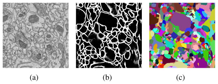
As shown in figure 1(b), the membrane detection output is a probability map, on which we can simply apply thresholding to get a segmentation. However, small mispredictions about membranes in pixels could lead to significant under-segmentation errors. To address this problem, we propose a watershed tree based method. Consider a probability map as a 3D terrain map with pixel probability as ridge height. Regions with low probabilities make an initial segmentation as shown in figure 1(c). With the water level rising, small regions merge into larger ones, and finally into one large region with the water level above the highest ridge in the map. This technique produces a hierarchy of segmentations that can be represented by a tree structure, which we call a watershed merge tree.
Figure 1.

Example of (a) original EM image, (b) membrane detection and (c) initial watershed segmentation.
A watershed merge tree T = ({N}, {E}) is defined as a representation of region merging hierarchy: a node at depth d corresponds to an image region ; an edge from a parent node to its child node means region is a subregion of region ; a local tree structure ( , …) represents region can be the merging result of all of its subregion { , …}. For simplicity, we here consider the merge tree as a binary tree.
An initial water level l0 is used to merge some very small regions beforehand in the initial segmentation, and a preprocessing is conducted to remove regions smaller than nr pixels by merging them with their neighbor regions that have the lowest probability barrier.
3. Boundary Classifier
In order to make decisions in a merge tree, we need to know how confident we are about whether each potential merge could happen. A boundary classifier is trained to give a prediction. Our classifier takes a set of 141 features extracted from the two merging regions, including geometric features (region area, boundary lengths, region contour lengths, etc.) and image statistics features for boundary pixels (intensity statistics) and regions (EM image texton histogram and watershed region merging saliency) from original EM images and membrane detection maps. Here, pixels adjacent to another region are considered as boundary pixels. The watershed region merging saliency is defined as the difference between the minimum water level it takes to merge the two regions and the minimum value in the membrane detection probability map.
Labels indicating whether a region pair should merge or keep split are obtained by measuring the Rand error over the ground truth segmentation (see section 5). A random forest classifier [4] is trained with corresponding weights assigned to positive/negative examples so as to balance their contributions. For the testing data, the trained classifier is applied to make a prediction about how likely a region pair should merge.
4. Resolving Merge Tree
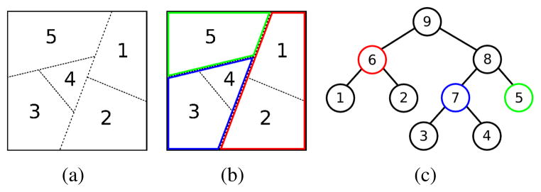
The boundary classifier predicts the probability for every potential merge in a merge tree, but this is not sufficient for generating a consistent segmentation of the whole image. We still need to resolve the tree in an optimization sense while preserving the consistency. We define consistency such that any pixel should be only labeled once. In other words, if a node in the merge tree is selected, all of its ancestors and descendants cannot be selected. Figure 2 shows an artificial example. The watershed algorithm generates an initial segmentation shown in figure 2(a), from which a merge tree is built as in figure 2(c). Node 5, 6 and 7 are selected for a consistent final segmentation as shown in figure 2(b). Consequently, the other nodes cannot be picked, because we can never have both the red region (node 6) and region 1 (or 2) at the same time, otherwise region 1 (or 2) would be labeled more than once as 1 (or 2) and 6, which is inconsistent by our definition.
Figure 2.

Example of (a) initial segmentation, (b) consistent final segmentation and (c) corresponding merge tree.
Let us consider a certain region in the final segmentation: it exists because it neither splits into smaller regions nor merges with others into a larger region. Since each prediction that the classifier makes depends only on the two merging regions, we compute the possibility that a node is picked for the final segmentation as the probability that its two child nodes and merge and at the same time does not merge with its sibling node at the next higher water level to their parent node . We define a potential for as
| (1) |
where is the predicted probability that the two child nodes and merge (see section 3), and is the probability that node merge with its sibling node . In the example shown in figure 2(c), the potential of node 6 is P6 = p1,2(1 − p6,8). Since leaf nodes have no children, their potentials are defined as the probability that they do not merge penalized into half. Similarly, the root node has no parent, so its potential is half of the probability that its children will merge.
In this way, every node in the merge tree is assigned a potential, and the next step is to select a subset of the nodes to form a complete consistent segmentation. Here we use a greedy approach. The node with the highest potential in the merge tree is picked. Then all of its ancestors and descendants are regarded as inconsistent choices and removed from the tree. This procedure is repeated until there are no nodes left in the tree. The set of all the picked nodes makes up a complete consistent final segmentation.
5. Experimental Results
We use a set of 70 700 × 700 mouse cerebellum EM images (one slice shown in figure 1(a)) along with the corresponding ground truth images annotated manually by an expert. These images are divided into five bins randomly with 14 images in each bin. A multi-context MLP-ANN classifier [9] is trained with bin 1, and used for membrane detection for the other four bins. To test our method, we train the boundary classifier with four bins consisting of bin 1 and three bins out of bin 2 to 5. Then we test on the remaining one bin.
With the membrane probability maps, initial watershed segmentations are generated and merge trees are built. The initial water level l0 for each image is set as one percent of the maximum value in the corresponding probability map. Regions smaller than nr = 50 pixels are removed in the initial segmentations. 7 × 7 texture patches are extracted from the EM images for generating the texton dictionary and building texton histograms as boundary classifier features. A random forest with 255 trees is trained for boundary classification.
To train a boundary classifier, we assign a label from ground truth segmentations that indicates if a region pair ( ) should merge or not. We use the Rand error to measure whether two regions should merge. It is defined as
| (2) |
where (xp, xq) represents any pixel pair from the union of the two merging regions, and
| (3) |
| (4) |
| (5) |
The label indicating merge/split for ( ) is decided as
| (6) |
In this way, all the labels for the training data are generated automatically.
We also use Rand error as the measurement of segmentation quality. The Rand errors of the segmentations, obtained via thresholding the membrane detection probability maps with a best threshold for each bin respectively, are computed as comparison with our method. The results are shown in table 1, from which we can see that our method improves the segmentation substantially by reducing classification mistakes over more than 10 percent of the total pixel pairs.
Table 1.
Segmentation Rand errors. (TH: thresholding; MT: merge tree method).
| bin 2 | bin 3 | bin 4 | bin 5 | avg. | |
|---|---|---|---|---|---|
| TH | 0.2749 | 0.2419 | 0.2115 | 0.2717 | 0.2500 |
| MT | 0.1529 | 0.1113 | 0.1029 | 0.1595 | 0.1316 |
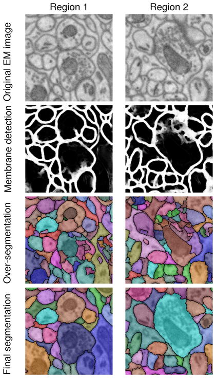
Figure 3 shows some visual results of our test images. Our approach for resolving the watershed merge tree can make most initial over-segmentations merge accurately, and the complete method gives a good final segmentation.
Figure 3.
Segmentation results of two image regions (zoomed in).
Contributor Information
Ting Liu, Email: ting@sci.utah.edu.
Elizabeth Jurrus, Email: liz@sci.utah.edu.
Mojtaba Seyedhosseini, Email: mseyed@sci.utah.edu.
Mark Ellisman, Email: mark@ncmir.ucsd.edu.
Tolga Tasdizen, Email: tolga@sci.utah.edu.
References
- 1.Andres B, Köthe U, Helmstaedter M, Denk W, Hamprecht F. Segmentation of SBFSEM volume data of neural tissue by hierarchical classification. Pattern recognition. 2008:142–152. [Google Scholar]
- 2.Arbelaez P. Boundary extraction in natural images using ultrametric contour maps. Computer Vision and Pattern Recognition Workshop, 2006. CVPRW’06. Conference on; Ieee; 2006. pp. 182–182. [Google Scholar]
- 3.Arbelaez P, Maire M, Fowlkes C, Malik J. Contour detection and hierarchical image segmentation. Pattern Analysis and Machine Intelligence, IEEE Transactions on. 2011;(99):1–1. doi: 10.1109/TPAMI.2010.161. [DOI] [PubMed] [Google Scholar]
- 4.Breiman L. Random forests. Machine learning. 2001;45(1):5–32. [Google Scholar]
- 5.Briggman K, Denk W. Towards neural circuit reconstruction with volume electron microscopy techniques. Current opinion in neurobiology. 2006;16(5):562–570. doi: 10.1016/j.conb.2006.08.010. [DOI] [PubMed] [Google Scholar]
- 6.Funke J, Andres B, Hamprecht F, Cardona A, Cook M. Multi-hypothesis CRF-segmentation of neural tissue in anisotropic em volumes. Arxiv preprint arXiv:1109.2449. 2011 [Google Scholar]
- 7.Jain V, Murray J, Roth F, Turaga S, Zhigulin V, Briggman K, Helmstaedter M, Denk W, Seung H. Supervised learning of image restoration with convolutional networks. Computer Vision, 2007. ICCV 2007. IEEE 11th International Conference on; IEEE; 2007. pp. 1–8. [Google Scholar]
- 8.Jurrus E, Paiva A, Watanabe S, Anderson J, Jones B, Whitaker R, Jorgensen E, Marc R, Tasdizen T. Detection of neuron membranes in electron microscopy images using a serial neural network architecture. Medical Image Analysis. 2010;14(6):770–783. doi: 10.1016/j.media.2010.06.002. [DOI] [PMC free article] [PubMed] [Google Scholar]
- 9.Seyedhosseini M, Kumar R, Jurrus E, Giuly R, Ellisman M, Pfister H, Tasdizen T. Detection of neuron membranes in electron microscopy images using multi-scale context and radon-like features. Medical Image Computing and Computer-Assisted Intervention–MICCAI 2011. 2011:670–677. doi: 10.1007/978-3-642-23623-5_84. [DOI] [PMC free article] [PubMed] [Google Scholar]
- 10.Sporns O, Tononi G, Kötter R. The human connectome: a structural description of the human brain. PLoS Computational Biology. 2005;1(4):e42. doi: 10.1371/journal.pcbi.0010042. [DOI] [PMC free article] [PubMed] [Google Scholar]


