Bayesian Proteoform Modeling Improves Protein Quantification of Global Proteomic Measurements

Abstract

As the capability of mass spectrometry-based proteomics has matured, tens of thousands of peptides can be measured simultaneously, which has the benefit of offering a systems view of protein expression. However, a major challenge is that, with an increase in throughput, protein quantification estimation from the native measured peptides has become a computational task. A limitation to existing computationally driven protein quantification methods is that most ignore protein variation, such as alternate splicing of the RNA transcript and post-translational modifications or other possible proteoforms, which will affect a significant fraction of the proteome. The consequence of this assumption is that statistical inference at the protein level, and consequently downstream analyses, such as network and pathway modeling, have only limited power for biomarker discovery. Here, we describe a Bayesian Proteoform Quantification model (BP-Quant)¹ that uses statistically derived peptides signatures to identify peptides that are outside the dominant pattern or the existence of multiple overexpressed patterns to improve relative protein abundance estimates. It is a research-driven approach that utilizes the objectives of the experiment, defined in the context of a standard statistical hypothesis, to identify a set of peptides exhibiting similar statistical behavior relating to a protein. This approach infers that changes in relative protein abundance can be used as a surrogate for changes in function, without necessarily taking into account the effect of differential post-translational modifications, processing, or splicing in altering protein function. We verify the approach using a dilution study from mouse plasma samples and demonstrate that BP-Quant achieves similar accuracy as the current state-of-the-art methods at proteoform identification with significantly better specificity. BP-Quant is available as a MatLab® and R packages.

The application of MS-based proteomics has resulted in large-scale studies in which the set of measured, and subsequently identified, peptides is often used to estimate protein abundance. In particular, label-free MS-based proteomics is highly effective for identification of peptides and measurement of relative peptide abundances (1, 2), but it does not directly yield protein quantities. The importance of accurate protein quantification cannot be understated; it is the essential component of identifying biomarkers of disease or defining the relationship between gene regulations, protein interactions, and signaling networks in a cellular system (3, 4). The major challenge is that protein abundance depends not only on transcription rates of the gene but also on additional control mechanisms, such as mRNA stability, translational regulation, and protein degradation. Moreover, the functional activity of proteins can be altered through a variety of post-translational modifications or proteolytic processing and alternative splicing, events which selectively alter the abundance of some selected peptides while leaving others unchanged (4). This complexity of the proteome, in addition to issues associated with the measurement and identification errors, presents a significant challenge to accurate relative protein quantification (5).

Smith et al. (3) recently described the importance of capturing protein variation in all forms (e.g. post-translational modifications, splice variants), all of which are collectively referred to as proteoforms. To date, little has been described in respect to automated identification of proteoforms. Most work on improving protein quantification for label-free data focuses on removing variation from the data through peptide filtering, such as removing shared peptides or those that do not meet frequency and coefficient of variation (CV) thresholds (6). Several recent methodologies have described approaches to deal with shared peptides either through linear programming (7), hierarchical modeling (8), or peptide detectability (9) to improve protein-level quantification. However, these approaches do not identify or quantify distinct proteoforms of a protein. The current state-of-the-art method for proteoform discovery uses a combination of correlation and clustering to identify distinct patterns (10). Protein quantification by peptide quality control (PQPQ) to date has only been applied to labeled data but is generic and can be applied to label-free experiments as well.

Generating a parsimonious protein list is a well-known practice in protein inference. The procedure involves assembling the most concise set of proteins across the assigned peptide sequences observed in an experiment (11). We present the novel approach of statistically informed peptide selection using a Bayesian proteoform quantification (BP-Quant) approach for parsimonious, relative protein quantification (Fig. 1). Research objectives are at the foundation of BP-Quant. Peptides to be used for protein quantification are selected using a peptide-specific signature vector that is determined by statistical hypothesis tests relevant to the research objective(s) of the experiment as well as the directionality of the effect(s) (i.e. upward or downward abundance). The statistical signature-based approach does not omit shared peptides, although it does not directly account for the fact that a peptide is shared. BP-Quant-based protein quantification is a multi-step process that (1) generates the peptide signature vectors based on the research hypotheses, (2) assigns probabilities to potential proteoform configurations, and (3) selects peptides with an over-representation of a similar signature to be used for relative protein abundance estimates.

Fig. 1.

BP-Quant for parsimonious protein quantification is driven by research objectives that define statistical patterns of interest. Relative protein abundance values are estimated using peptides that share similar statistical behavior.

EXPERIMENTAL PROCEDURES

Discovery of candidate plasma biomarkers is of interest to many applications, such as disease specificity, drug toxicity, drug response, and fundamental research (12–15). Plasma samples collected from standard inbred mice under the National Institutes of Health National Institute of Environmental Health Sciences Biomarkers of Exposure project (http://www.niehs.nih.gov/health/topics/science/biomarkers/) were used for a dilution study. Although the focus of this larger project was to understand the development and progression of complex disease due to exposure to environmental stressors in the presence of risk factors such as obesity or exposure to inhaled endotoxins (e.g. lipopolysaccharide) (16), here we constructed an experiment that yields expected protein ratios and for which known concentrations can be used to define datasets with positive examples (proteins with multiple proteoforms) and negative examples (proteins with a single proteoform).

Sample Preparation

Mouse plasma samples (n = 16) were previously depleted of the seven most abundant proteins using an IgY7 depletion column and digested using the approach described in Zhou et al. (17). For this dilution study, the digested mouse plasma samples were spiked with an amount of digested Shewanella oneidensis MR-1 to maintain a constant peptide concentration for MS analysis. Each of the 16 depleted and digested mouse plasma peptide samples and one S. oneidensis MR-1 peptide sample were assayed with bicinchoninic acid (Thermo Scientific, Rockford, IL) to determine the peptide concentration. The 16 mouse plasma samples were then subjected to four dilutions; (1) 1:0 mouse: S. oneidensis, (2) 1:1 mouse: S. oneidensis, (3) 1:3 mouse: S. oneidensis; and (4) 1:7 mouse: S. oneidensis. Each sample was vortexed and made to a final concentration of 0.25 μg/μl using 25 mm ammonium bicarbonate, pH 8.0. All samples were assayed again with bicinchoninic acid to ensure accuracy.

Reversed-Phase Capillary LC-MS Analyses

Diluted peptide samples (64 total = 16 samples by four dilutions), analyzed in duplicate, were balanced and randomized across a four-column custom-built capillary LC system coupled online to a LTQ-Orbitrap Velos mass spectrometer (Thermo Scientific, San Jose, CA) by way of an in-house manufactured electrospray ionization interface, as previously described (18). Electrospray emitters were custom made using 150 μm outer diameter × 20 μm inner diameter chemically etched fused silica capillaries, as previously described (19). Reversed-phase capillary columns were prepared by slurry packing 3-μm Jupiter C18 bonded particles (Phenomenex, Torrance, CA) into a 75 μm × 65 cm fused silica capillary (Polymicro Technologies, Phoenix, AZ) using 0.5 cm sol-gel plugs for particle retention (20). Mobile phases consisted of (a) 0.1% formic acid in water and (b) 0.1% formic acid in acetonitrile and were degassed on-line using a Degasys Model DG-2410 vacuum degasser (Dionex, Germany); the HPLC system was equilibrated at 10,000 psi with 100% mobile phase (a) for initial starting conditions. After loading 2.5 μg of peptides onto the column, the mobile phase was held at 100% mobile phase (a) for 50 min. Exponential gradient elution was initiated 50 min after sample loading with an initial column flow rate of 400 nl/min, and the mobile phase was ramped from 0% to 55% mobile phase (b) over 100 min using a 2.5 ml stainless steel mixing chamber, followed by a rapid increase to ∼100% (b) for 10 min to wash the column. The temperature of the heated capillary and the electrospray ionization voltage were 200 °C and 2.2 kV, respectively. Data were collected over the mass range 400–2,000 m/z.

Peptide Identification

Quantitative LC-MS data were processed using the PRISM Data Analysis system (21), which is a series of software tools developed in-house (e.g. Decon2LS (22) and VIPER (23). The first step involved deisotoping of the raw MS data to give the monoisotopic mass, charge state, and intensity of the major peaks in each mass spectrum (22). The data were next examined in a two-dimensional fashion to identify groups of mass spectral peaks observed in sequential spectra using an algorithm that computes a Euclidean distance in n-dimensional space for combinations of peaks (23). Each group, generally ascribed to one detected species and referred to as an “LC-MS feature,” has a median monoisotopic mass, central normalized elution time (NET), and abundance estimate computed by summing the intensities of the MS peaks that comprise the entire feature. The peptide identities of detected features in each dataset (here a dataset is equivalent to a single LC-MS analysis) was determined by comparing their measured monoisotopic masses and NETs to the calculated monoisotopic masses and observed NETs of each of the peptides in a mouse plasma/Shewanella accurate mass and time tag database (24) within initial search tolerances of ± 6 ppm and ± 0.025 NET for monoisotopic mass and elution time, respectively. The peptides identified from this matching process were retained as a matrix for subsequent data analysis and are available in Excel format in supplementary data and online at http://omics.pnl.gov/view/publication_1088.html.

Statistical Preprocessing of Peptide Abundance Dataset

Peptide abundance data were transformed to the log₂ scale, and missing data values were left as blank (not imputed) prior to processing. Peptides with an insufficient amount of data to perform a qualitative or quantification statistical difference test (e.g. G-test or Analysis of Variance (ANOVA)) across the set of biological replicates were removed (25). The full collection of mouse plasma and S. oneidensis peptides were evaluated for evidence of unusual peptide abundance distributions across the pool of LC-MS analyses (26). The peptides associated with the mouse plasma were extracted, technical replicates were averaged, and additional peptide filtering was performed to ensure sufficient data across the pool of samples. The mouse plasma data were normalized using a two-step process. First, the undiluted samples consisting of only mouse peptides (0.50 μg/μl, n = 16) were mean centered using a rank invariant peptide subset (27). The remaining three dilution sets (0.25 μg/μl, 0.125 μg/μl, and 0.0625 μg/μl) were then normalized as a function of the expected dilution ratio to the normalized peptide set consisting of only mouse peptides.

BP-Quant

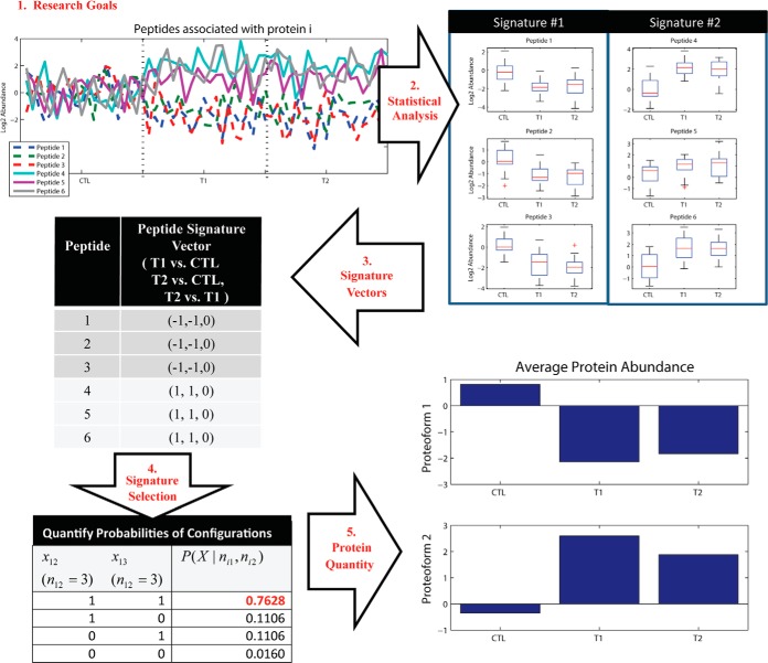
Fig. 2 presents an example of the BP-Quant approach to protein quantification. Step 1 defines the research goal, for example, identifying proteins with any statistically significant differential expression (i.e. abundance) between control and two conditions (T1 and T2). Step 2 treats each peptide as an independent source of information and evaluates each using an appropriate statistical test, such as an ANOVA with a Tukey's post-hoc test to adjust for the multiple comparisons within the peptide (28). In Step 3, the statistical results, typically p values, are translated into signatures based on the trinary descriptors (-1, 0, or 1) where -1 and 1 indicate the treatment group has lower or higher expression, respectively, than the comparison group and 0 indicates no statistical difference in peptide abundance. In particular, the significant features are checked for each individual contrast such as (1) control versus T1, (2) control versus T2, and (3) T1 versus T2. In practice, the primary signature vector is based on the comparison of quantitative peptide abundance values across groups, where groups are defined by the research objectives. A secondary signature vector can also be defined based on the comparison of the frequency of response (i.e. presence/absence) across comparison groups, which is highly relevant for proteomics data given the large fraction of missing values. If the primary signature vector lacks a p-value which indicates inadequate data for a quantitative statistical test, then they are replaced using the corresponding secondary signature vector value(s) that are based on qualitative test results. The fourth step computes the probability of all possible proteoform configurations, thus identifying how many proteoforms are present and the peptides associated with each proteoform. The last step then quantifies protein-level expression using standard approaches (29).

Fig. 2.

A demonstration of the overall BP-Quant approach using simulated data to represent a protein k with six peptides categorized into two unique statistical vectors. The BP-Quant algorithm generates peptide signature vectors using the results of statistical analyses which are defined by the research objectives (Steps 1, 2, and 3). The peptide signature vectors are binned by uniqueness and tallied (Step 4) and quantified into unique protein estimates (proteoforms).

Bayesian Peptide Selection/Proteoform Identification

The goal of the Bayesian inference problem is to determine a specific proteoform configuration given the information for protein i. We assume that each unique peptide signature can result in a unique proteoform, and thus, each signature is defined as a Bernoulli random variable where x_ij = 1 if proteoform j is present for protein i and 0 otherwise. For each protein i, we observe a count for signature j (n_ij) and similar to prior work in protein inference (30, 31), the goal is to determine the maximum a posteriori (MAP) proteoform configuration, which is dependent upon the observed signature counts:

The MAP proteoform configuration (Eq. 1) is found by evaluating the posterior probability of each configuration where all random variables are described in Table I:

Table I. Notations and definitions.

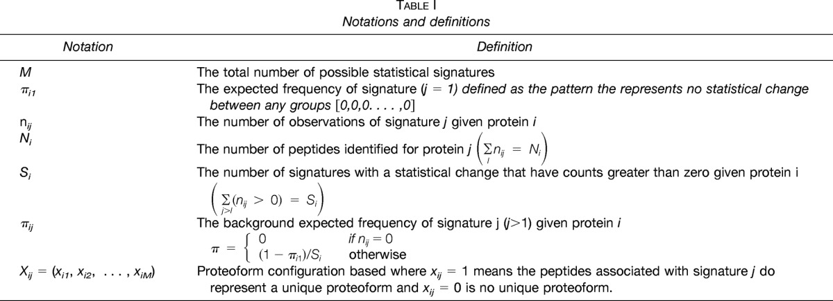
The probability that we would observe a specific number of peptides displaying signature j for protein i is dependent upon the proteoform configuration for that signature. Under the assumption that each signature is independent, we can simplify Eq. 2 to

where X_i=[x_i1, x_i2, , x_iJ]. In practice, the assumption of independence of peptides will not hold holistically; however, this assumption works relatively well for initial model development similar to protein inference. We model the probability that we would observe a specific number of observations for a given signature as a binomial distribution. For example, if we have a background frequency (π) of 0.15 for signature j of protein i, there is only a 2.1% chance that we would observe this signature four or more times for a protein containing eight peptides. If the proteoform is present, x_ij is one, we sum over the binomial probabilities from the lower tail of a binomial. Thus, if the likelihood of observing n_ij by chance is very low, the probability in the lower tail will be high. We utilize this distributional information to determine the likelihood of over-represented signatures that are indicative of a proteoform. Since x is binary, the prior, P(x_ij, is modeled as a Bernoulli random variable;

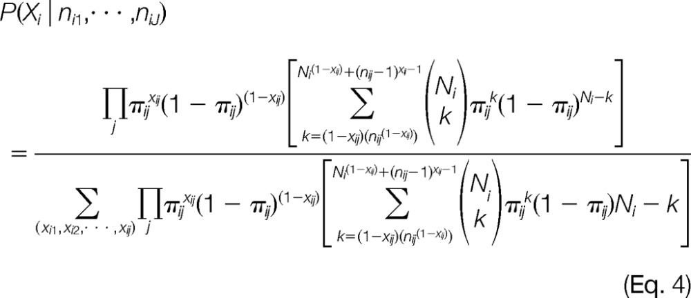The computational time to solve Eq. 4 is minimal because the full possible set of solutions for X_i is constrained by the observed signatures within protein i. Therefore, we only consider a small subset of all possible proteoform configurations. Equation 4 is used to compute the probabilities of the possible proteoform configurations (Step 4) in Fig. 2, and the final step then uses the peptides assigned to each proteoform to infer a protein-level estimate.

The probabilistic inference of proteoform configurations is dependent upon the expected background frequency of each signature π_ij. A data-driven approach is used to infer this probability by defining random dataset(s) with the same properties as the data to be evaluated but defined to have no statistical changes between groups. Each dataset is generated by simulating data for each peptide in the original data as a normal random variable with a mean of 0 and the pooled estimate of variance from the observed data. Values for the peptide are then removed at random to yield the same amount of missing values from the peptide as observed in the real data. Once all peptides have been simulated Steps 1–3 of the BP-Quant protocol are performed. For the dataset, we define α_I, as the total number of peptides identified to have a single proteoform divided by the total number of peptides. We repeat the process 100 times to identify a robust estimate of π₁ as the average across all αs. The estimate of π_ij is based upon π₁, and the total number of signatures as defined in Table I.

RESULTS

To explore the capability of BP-Quant to correctly identify the number of proteoforms associated with a protein we use the dilution series, which consists of 100 proteins where each protein contains from 2 to 188 peptides. We compare these results to a standard correlation-based approach (PQPQ) that uses clusters defined from correlation to define proteoforms (10, 32). We used the publicly available version of PQPQ, which runs in MATLAB 2013a with all defaults. Since the PQPQ software is designed for labeled data, we defined the highest dilution as our control set and allowed PQPQ to perform the analysis on the ratios to this group. For consistency, the peptide relationships to proteins and proteoforms were extracted from the output, and protein quantification was performed identical to BP-Quant using a reference-based approach—R-Rollup (29, 33).

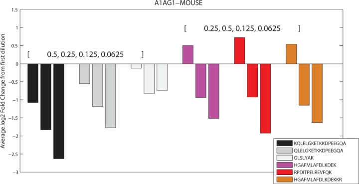
The dilution series dataset in its native state has no biological variability, and therefore, every protein should have only a single proteoform. BP-Quant indeed identified a single proteoform state as the most probable for each protein. PQPQ identifies 5% of the proteins as having more than one proteoform. To evaluate performance in respect to accuracy and sensitivity, datasets for which proteins are defined where the exact number of proteoforms is known are required. This can be constructed with exact knowledge from the dilution series. As an example, imagine a protein in the dilution series with six peptides. The first three peptides maintain the basic order of [0.5, 0.25, 0.125, 0.0625], thus the pattern is a clear decrease from the 0.5 dilution. The next three peptides have the dilution [0.25, 0.5, 0.125, 0.0625], and thus, the expression pattern is an initial increase from 0.25 followed by a decrease for the last two dilutions. In this example (Fig. 3), these are the six peptides and associated abundance values identified from protein A1AG1_mouse, for which simply the last three peptides were permuted to the second dilution ordering. Therefore, for this protein, we can clearly define that we have two distinct proteoforms. For every protein in the dilution series, we first select a defined number of proteoforms, second identify which peptides will belong to each proteoform (minimum of three), and lastly determine the dilution ordering (permutation) for each proteoform. To assess variability in the final result, we generate the complete dataset 50 times.

Fig. 3.

Example of defined proteoform state for a specific protein using dilution permutation to generate datasets with positive and negative proteoform examples.

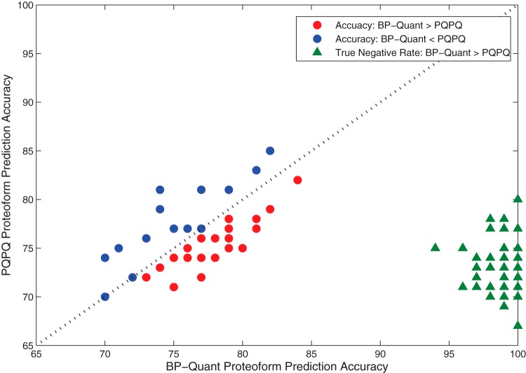
Across the 50 datasets, there were on average 42 ± 3.5 proteins (of 100 total) with multiple proteoforms, and the number of proteoforms for these proteins ranged from 2–6 (average of 3.1). For each of the datasets, the predicted number of proteoforms to the known number of proteoforms was compared, and the accuracy was quantified. The accuracy was defined based on true positive (TP) and true negatives (TN) where TP and TN are the total the number of proteins that correctly identified the number of proteoforms—(TP+TN)/100. Alternately, metrics such as root mean square error can be used but return similar results (data not shown). Fig. 4 shows a comparison of BP-Quant versus PQPQ with respect to accuracy for each of the 50 datasets (circles). The accuracies are relatively similar, average of 76.7% and 76.0%, with standard deviations of 3.3% and 3.3%, for BP-Quant and PQPQ, respectively. In 64% of the cases, BP-Quant had a higher accuracy, which was statistically significant by a Wilcoxon rank sum test (p ∼0.007).

Fig. 4.

The accuracy of BP-Quant versus PQPQ for the positive (circles) and negative (triangles) constructed datasets.

The measure of accuracy in Fig. 4 does not directly consider the specificity of the test, i.e. the number of times a protein with a single proteoform (TN) is falsely identified as having multiple proteoforms, a false positive (FP), or conversely, a false negative (FN). Thus, we also evaluate the F1-score, which is the harmonic mean of precision and sensitivity; (2TP/2TP+FP+FN. Under the circumstance of no false identifications, the F1-score will be 1 and will decrease as the number of false positives and negatives increase. BP-Quant has a significantly higher F1-score than PQPQ based on a Wilcoxon signed rank test (p < 3e-4), larger in 74% of the datasets. Fig. 5 shows the confidence interval for the F1-score for each approach as well as a box plot of the difference inset in the figure.

Fig. 5.

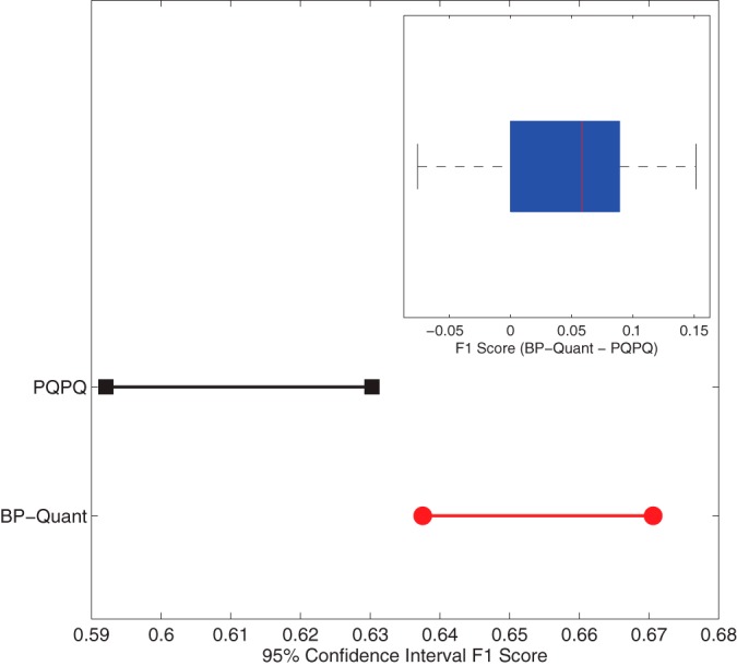
Confidence intervals of the F1-score for each approach and the measured difference across the 50 datasets (inset).

Lastly, to explore the impact of noisy data with no proteoform present, we used the dilution series data to construct negative sets by simply randomly permuting the data for each peptide and leaving the dilution ordering constant. In this manner, there should be no statistical difference between groups and those for which this is the case would be outliers. The accuracy of BP-Quant on this negative set is displayed in Fig. 4 (green triangles). The average accuracy of BP-Quant on the negative set was 98.5% with a standard deviation of 1.25% while PQPQ resulted in an average accuracy of only 72.9% with a standard deviation of 2.64%. This is similar to the observations for the dilution series with no permutations where PQPQ found 5 of the 54 proteins (>10%) were identified to have multiple proteoforms when only one proteoform is possible.

DISCUSSION

The use of proteomic measurements for biomarker discovery results in a vast amount of information that, by necessity, requires summarization to facilitate further biological conclusions. There is great benefit to a rigorous statistical investigation of the data in the context of the research hypothesis and the subsequent peptide and protein information available for biological modeling. Statistically informed peptide selection is essential for any of the relative protein quantification approaches presented when dealing with complex samples, such as those used in environmental, medical, or clinical studies. Such approaches are particularly important for lower abundances species, which are often of greatest interest in biomarker discovery efforts. In addition, since BP-Quant is a signature-based peptide selection methodology, it can be used as a precursor to any desired protein quantification method (e.g. reference-based or linear models).

Proteoform identification is one of the major challenges of the protein quantification field and is a necessity to facilitate biomarker discovery and improve fundamental knowledge of biological systems at the pathway level (3). The BP-Quant approach facilitates the discovery of significant biological patterns in the presence of substantial noise and also facilitates the discovery of multiple significant biological patterns (i.e. possible proteoforms), by selecting specific peptides that display unique patterns of expression. In many cases, such specific proteoforms, such as those arising from post-translational modifications, have been identified as associated with diseases such as Alzheimer's and Parkinson's (34). BP-Quant showed excellent specificity and similar accuracy to a correlation-based clustering approach to proteoform identification. The current implementation of BP-Quant assumes that peptides are independent, which clearly is not the case. Future explorations will evaluate using protein-level information, such as exon structure or peptide sequence overlap, or correlation, such as PQPQ, to identify these dependences and model them in the Bayesian framework.

In the absence of the BP-Quant approach, biologists have been presented with a sort of “consensus behavior” of the peptides mapped to a given protein, even as individual peptides may have been significantly modified as a specific response to experimental conditions. Because BP-Quant has the ability to effectively segregate the consensus peptides from the uniquely altered peptides, biologists can begin to assess the functional significance of specific proteoforms within a biological context. This is a powerful tool for systems biology studies in which the flow of information is as important as mere changes in abundance. It may also convey an additional layer of specificity on biomarker discovery efforts, greatly improving the ability to identify proteoform-specific biomarkers.

REFERENCES

- 1. Baker E. S., Liu T., Petyuk V. A., Burnum-Johnson K. E., Ibrahim Y. M., Anderson G. A., Smith R. D. (2012) Mass spectrometry for translational proteomics: progress and clinical implications. Genome Med. 4, 63. [DOI] [PMC free article] [PubMed] [Google Scholar]
- 2. Gillette M. A., Carr S. A. (2013) Quantitative analysis of peptides and proteins in biomedicine by targeted mass spectrometry. Nat. Methods 10, 28–34 [DOI] [PMC free article] [PubMed] [Google Scholar]
- 3. Smith L. M., Kelleher N. L. (2013) Proteoform: a single term describing protein complexity. Nat. Methods 10, 186–187 [DOI] [PMC free article] [PubMed] [Google Scholar]
- 4. Waters K. M., Pounds J. G., Thrall B. D. (2006) Data merging for integrated microarray and proteomic analysis. Brief Funct. Genomic Proteomic 5, 261–272 [DOI] [PubMed] [Google Scholar]
- 5. Goh W. W., Lee Y. H., Chung M., Wong L. (2012) How advancement in biological network analysis methods empowers proteomics. Proteomics 12, 550–563 [DOI] [PubMed] [Google Scholar]
- 6. Lai X., Wang L., Tang H., Witzmann F. A. (2011) A novel alignment method and multiple filters for exclusion of unqualified peptides to enhance label-free quantification using peptide intensity in LC-MS/MS. J. Proteome Res. 10, 4799–4812 [DOI] [PMC free article] [PubMed] [Google Scholar]
- 7. Dost B., Bandeira N., Li X., Shen Z., Briggs S. P., Bafna V. (2012) Accurate mass spectrometry based protein quantification via shared peptides. J. Comput. Biol. 19, 337–348 [DOI] [PMC free article] [PubMed] [Google Scholar]
- 8. Blein-Nicolas M., Xu H., de Vienne D., Giraud C., Huet S., Zivy M. (2012) Including shared peptides for estimating protein abundances: A significant improvement for quantitative proteomics. Proteomics 12, 2797–2801 [DOI] [PubMed] [Google Scholar]
- 9. Tang H., Arnold R. J., Alves P., Xun Z., Clemmer D. E., Novotny M. V., Reilly J. P., Radivojac P. (2006) A computational approach toward label-free protein quantification using predicted peptide detectability. Bioinformatics 22, e481–e488 [DOI] [PubMed] [Google Scholar]
- 10. Forshed J. (2013) Protein quantification by peptide quality control (PQPQ) of shotgun proteomics data. Methods Mol. Biol. 1023, 149–158 [DOI] [PubMed] [Google Scholar]
- 11. Zhang B., Chambers M. C., Tabb D. L. (2007) Proteomic parsimony through bipartite graph analysis improves accuracy and transparency. J. Proteome Res. 6, 3549–3557 [DOI] [PMC free article] [PubMed] [Google Scholar]
- 12. Senapati S., Barnhart K. T. (2013) Biomarkers for ectopic pregnancy and pregnancy of unknown location. Fertil. Steril.99, 1107–1116 [DOI] [PMC free article] [PubMed] [Google Scholar]
- 13. Chung L., Baxter R. C. (2012) Breast cancer biomarkers: proteomic discovery and translation to clinically relevant assays. Expert Rev. Proteomics 9, 599–614 [DOI] [PubMed] [Google Scholar]
- 14. Galasko D., Golde T. E. (2013) Biomarkers for Alzheimer's disease in plasma, serum and blood - conceptual and practical problems. Alzheimers Res. Ther. 5, 10. [DOI] [PMC free article] [PubMed] [Google Scholar]
- 15. Pin E., Fredolini C., Petricoin E. F., 3rd (2013) The role of proteomics in prostate cancer research: biomarker discovery and validation. Clin. Biochem. 46, 524–538 [DOI] [PubMed] [Google Scholar]
- 16. Tilton S. C., Waters K. M., Karin N. J., Webb-Robertson B. J., Zangar R. C., Lee K. M., Bigelow D. J., Pounds J. G., Corley R. A. (2013) Diet-induced obesity reprograms the inflammatory response of the murine lung to inhaled endotoxin. Toxicol. Appl. Pharmacol. 267, 137–148 [DOI] [PMC free article] [PubMed] [Google Scholar]
- 17. Zhou J. Y., Petritis B. O., Petritis K., Norbeck A. D., Weitz K. K., Moore R. J., Camp D. G., Kulkarni R. N., Smith R. D., Qian W. J. (2009) Mouse-specific tandem IgY7-SuperMix immunoaffinity separations for improved LC-MS/MS coverage of the plasma proteome. J. Proteome Res. 8, 5387–5395 [DOI] [PMC free article] [PubMed] [Google Scholar]
- 18. Livesay E. A., Tang K., Taylor B. K., Buschbach M. A., Hopkins D. F., LaMarche B. L., Zhao R., Shen Y., Orton D. J., Moore R. J., Kelly R. T., Udseth H. R., Smith R. D. (2008) Fully automated four-column capillary LC-MS system for maximizing throughput in proteomic analyses. Anal. Chem. 80, 294–302 [DOI] [PMC free article] [PubMed] [Google Scholar]
- 19. Kelly R. T., Page J. S., Luo Q., Moore R. J., Orton D. J., Tang K., Smith R. D. (2006) Chemically etched open tubular and monolithic emitters for nanoelectrospray ionization mass spectrometry. Anal. Chem. 78, 7796–7801 [DOI] [PMC free article] [PubMed] [Google Scholar]
- 20. Maiolica A., Borsotti D., Rappsilber J. (2005) Self-made frits for nanoscale columns in proteomics. Proteomics 5, 3847–3850 [DOI] [PubMed] [Google Scholar]
- 21. Kiebel G. R., Auberry K. J., Jaitly N., Clark D. A., Monroe M. E., Peterson E. S., Tolic N., Anderson G. A., Smith R. D. (2006) PRISM: a data management system for high-throughput proteomics. Proteomics 6, 1783–1790 [DOI] [PubMed] [Google Scholar]
- 22. Jaitly N., Mayampurath A., Littlefield K., Adkins J. N., Anderson G. A., Smith R. D. (2009) Decon2LS: An open-source software package for automated processing and visualization of high resolution mass spectrometry data. BMC Bioinformatics 10, 87. [DOI] [PMC free article] [PubMed] [Google Scholar]
- 23. Monroe M. E., Tolic N., Jaitly N., Shaw J. L., Adkins J. N., Smith R. D. (2007) VIPER: an advanced software package to support high-throughput LC-MS peptide identification. Bioinformatics 23, 2021–2023 [DOI] [PubMed] [Google Scholar]
- 24. Zimmer J. S., Monroe M. E., Qian W. J., Smith R. D. (2006) Advances in proteomics data analysis and display using an accurate mass and time tag approach. Mass Spectrom. Rev. 25, 450–482 [DOI] [PMC free article] [PubMed] [Google Scholar]
- 25. Webb-Robertson B. J., McCue L. A., Waters K. M., Matzke M. M., Jacobs J. M., Metz T. O., Varnum S. M., Pounds J. G. (2010) Combined statistical analyses of peptide intensities and peptide occurrences improves identification of significant peptides from MS-based proteomics data. J. Proteome Res. 9, 5748–5756 [DOI] [PMC free article] [PubMed] [Google Scholar]
- 26. Matzke M. M., Waters K. M., Metz T. O., Jacobs J. M., Sims A. C., Baric R. S., Pounds J. G., Webb-Robertson B. J. (2011) Improved quality control processing of peptide-centric LC-MS proteomics data. Bioinformatics 27, 2866–72 [DOI] [PMC free article] [PubMed] [Google Scholar]
- 27. Webb-Robertson B. J., Matzke M. M., Jacobs J. M., Pounds J. G., Waters K. M. (2011) A statistical selection strategy for normalization procedures in LC-MS proteomics experiments through dataset-dependent ranking of normalization scaling factors. Proteomics 11, 4736–4741 [DOI] [PMC free article] [PubMed] [Google Scholar]
- 28. Ott L., Longnecker M. (2008) An Introduction to Statistical Methods and Data Analysis. Brooks/Cole, Belmont [Google Scholar]
- 29. Matzke M. M., Brown J. N., Gritsenko M. A., Metz T. O., Pounds J. G., Rodland K. D., Shukla A. K., Smith R. D., Waters K. M., McDermott J. E., Webb-Robertson B. J. (2013) A comparative analysis of computational approaches to relative protein quantification using peptide peak intensities in label-free LC-MS proteomics experiments. Proteomics 13, 493–503 [DOI] [PMC free article] [PubMed] [Google Scholar]
- 30. Li Y. F., Arnold R. J., Li Y., Radivojac P., Sheng Q., Tang H. (2009) A Bayesian approach to protein inference problem in shotgun proteomics. J. Comput. Biol. 16, 1183–1193 [DOI] [PMC free article] [PubMed] [Google Scholar]
- 31. Serang O., Noble W. (2012) A review of statistical methods for protein identification using tandem mass spectrometry. Stat. Interface 5, 3–20 [DOI] [PMC free article] [PubMed] [Google Scholar]
- 32. Forshed J., Johansson H. J., Pernemalm M., Branca R. M., Sandberg A., Lehtio J. (2011) Enhanced information output from shotgun proteomics data by protein quantification and peptide quality control (PQPQ). Mol. Cell. Proteomics 10, M111 010264 [DOI] [PMC free article] [PubMed] [Google Scholar]
- 33. Polpitiya A., Qian W., Jaitly N., Petyuk V., Adkins J. N., Camp D. C., 2nd, Anderson G., Smith R. (2008) DAnTE: a statistical tool for quantitative analysis of -omics data. Bioinformatics 24, 1556–1558 [DOI] [PMC free article] [PubMed] [Google Scholar]
- 34. Choi J., Rees H. D., Weintraub S. T., Levey A. I., Chin L. S., Li L. (2005) Oxidative modifications and aggregation of Cu,Zn-superoxide dismutase associated with Alzheimer and Parkinson diseases. J. Biol. Chem. 280, 11648–11655 [DOI] [PubMed] [Google Scholar]