Joint radius-length distribution as a measure of anisotropic pore eccentricity: An experimental and analytical framework

Abstract

In this work, we present an experimental design and analytical framework to measure the nonparametric joint radius-length (R-L) distribution of an ensemble of parallel, finite cylindrical pores, and more generally, the eccentricity distribution of anisotropic pores. Employing a novel 3D double pulsed-field gradient acquisition scheme, we first obtain both the marginal radius and length distributions of a population of cylindrical pores and then use these to constrain and stabilize the estimate of the joint radius-length distribution. Using the marginal distributions as constraints allows the joint R-L distribution to be reconstructed from an underdetermined system (i.e., more variables than equations), which requires a relatively small and feasible number of MR acquisitions. Three simulated representative joint R-L distribution phantoms corrupted by different noise levels were reconstructed to demonstrate the process, using this new framework. As expected, the broader the peaks in the joint distribution, the less stable and more sensitive to noise the estimation of the marginal distributions. Nevertheless, the reconstruction of the joint distribution is remarkably robust to increases in noise level; we attribute this characteristic to the use of the marginal distributions as constraints. Axons are known to exhibit local compartment eccentricity variations upon injury; the extent of the variations depends on the severity of the injury. Nonparametric estimation of the eccentricity distribution of injured axonal tissue is of particular interest since generally one cannot assume a parametric distribution a priori. Reconstructing the eccentricity distribution may provide vital information about changes resulting from injury or that occurred during development.

I. INTRODUCTION

The shape and size distribution of pores strongly influence transport and material properties of porous media. Specifically, these morphological features are known to affect the macroscopic electrical conductivity, thermal conductivity, hydraulic permeability, solute and solvent diffusivity, as well as the mechanical stiffness, susceptibility to fracture, and many other properties. Pores that are not spherical and largely aligned with one another can result in macroscopic tensorial relationships between generalized flows or fluxes and forces.¹

In biology, shape and pore-size distribution (PSD) strongly influence macroscopic functional properties. In the nervous system, axons can be viewed as being impermeable cylindrical pores whose diameter is known to be correlated with the conduction velocity of nervous impulses.^2,3 In addition, the distribution of diameters of these axons, and thus the distribution of velocities of nerve impulses, is a determinant of the amount of information that can propagate along a bundle of the axonal fibers or a fascicle.⁴ Furthermore, quantification of the compartment shape eccentricity, in addition to its size, is particularly valuable in injured axons, as it is known to change following mechanical, chemical, or metabolic insults.^5–8 This local variation in eccentricity is usually referred to as “beaded” axonal morphology, and its noninvasive characterization is of great value in assessing the functional status of nervous tissue. In muscle, another fibrous tissue, the individual components that comprise the muscle fiber are long tubular cells (myocytes). Their length and cross-sectional area are proportional to the muscle functional properties, such as force and velocity.^9,10 Cortical bone is another biological porous material, which contains anisotropic anatomic cavities of different sizes.¹¹ These anatomic microstructural variations have a significant impact on the material properties of cortical bone^12,13 and are also known to be affected by age and disease.¹⁴ Finally, in plant biology, the sieve tubes, which are part of the phloem tissue that conducts nutrients, can be viewed as elongated cylindrical cells that are connected at the ends and separated by porous plates.¹⁵ It has been proposed that these sieve tube elements are critical in regulating water and nutrient flow, but a quantitative characterization of their structure and morphology is still lacking.¹⁶

MR provides many types of contrasts that can be used to determine features of pore microstructure and morphology. For instance, diffusion MR of spin-labeled mobile molecules within pores permit us to infer features of pore shape from their net displacement distribution and its dependence on diffusion time. The single pulsed-field gradient (s-PFG) experiment¹⁷ is most commonly used to obtain this size and shape information. This experiment consists of a single pair of magnetic field gradient pulses of duration δ, with a separation Δ embedded within a conventional Hahn spin-echo MR experiment. The restricting nature of pores can result in estimates of average pore size¹⁸ or macroscopic anisotropy.¹⁹

Special attention was given to different types of anisotropy by Özarslan,²⁰ as well as experimental and analytical strategies to measure them. The compartment shape anisotropy (CSA) of a capped cylinder geometry can be measured using a variant of the s-PFG MR experiment, the double-PFG (d-PFG).^21,22 In this case, two PFG pairs with amplitudes G₁ and G₂, and a prescribed relative angle between them, are applied successively, separated by a mixing time, τ_m. The d-PFG experiment is sensitized to the temporal correlations of molecular motion within the two diffusion periods and is sensitive to the direction of the applied gradients.²³ Using this experiment one can obtain the average pore size^24–26 and the microscopic anisotropy.²⁷ As the relative angle can be varied, 3D information regarding the restricting compartment can be obtained, including the CSA. In the case of a capped cylinder geometry, both radius and length would provide an exact estimate of eccentricity.²⁰

In most cases, the MR signal is generated from an ensemble of polydisperse pores. Estimating the PSD with an assumed parametric distribution has a long history.^28,29 This quantity can also be estimated empirically, without a priori information (i.e., non-parametrically) using s-PFG NMR in conjunction with solving a system of linear equations.³⁰ In this case, the stability and accuracy of the solution depend on the degree of linear independence of the columns of the transfer matrix (the matrix that describes the set of linear equations), which effectively measures the degree of correlation between the independent variables.^31,32 The solution to this inverse problem of estimating the PSD becomes more ill posed as the degree of linear dependence and condition number increase. In an attempt to stabilize PSD estimation, it was recently suggested that a d-PFG rather than a s-PFG experiment be used.³³ The former approach adds an independent second dimension to the parameter space that acts to constrain the estimates of pore shape and size. The theoretical benefits of the d-PFG in the context of PSD estimation were discussed and demonstrated,³³ along with strategies for optimal experimental design,³⁴ and later validated on calibrated cylindrical microcapillary phantoms, resulting in accurate PSD estimation.³⁵ This method was also applied to drug-releasing bioresorbable porous polymer films, resulting in the estimate of a continuous size distribution of spherical pores.³⁶

To date, PSD estimation has been obtained from pores assumed to be either infinite cylinders or spheres, both having an isotropic compartment shape. To derive a PSD of an ensemble of anisotropic pores, the system must be described by (at least) a bivariate size distribution instead of a one-size variable distribution. A finite (capped) cylinder, for instance, would be characterized by a 2D joint size distribution function (R-L distribution), consequently having a marginal radius distribution (MRD) and a marginal length distribution (MLD).

In the present study, we propose a framework to estimate the joint R-L distribution of a population of capped cylinders by encoding specific planes of the specimen using the d-PFG MR experiment. This unique experimental design allows us to derive separately the complex spatial information from the parallel and the perpendicular dimensions of the cylinder and then use this information to reconstruct the joint R-L distribution. Two simulated representative joint distribution phantoms corrupted by different noise levels were then used to reconstruct the ground-truth joint R-L distribution.

II. THEORY

To date, only isotropic shapes have been considered in the model that describes the nonparametric PSD.^30,35,36 In those cases, the general assumption was that the acquired signal is the superposition of the calculated signals originating from the different isotropic pores. The signal can be expressed as

$$E^{data}\left({\Omega }_k\right)=\sum _i\Psi \left(R_i\right)\mathbf{E}({\Omega }_k,R_i),$$ (1)

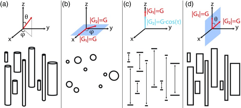
where Ψ(R_i) are the volumetric fractions, or the PSD, which satisfy ∑_iΨ(R_i) = 1. Ω_k is the kth experimental parameter set, i.e., a combination of G, δ, Δ, and the gradient direction, which in a spherical coordinate system is given by the polar and azimuthal angles θ and φ (Fig. 1(a), top). In this study, we consider the 3D parametric space that is formed solely by varying Δ, G, and φ/θ. Higher dimensional information (e.g., Δ₁ ≠ Δ₂ or variation of δ) can be easily incorporated into this framework. We introduce a new parameter, τ, according to which the amplitude of G₂ is varied in a z axis experiment (Fig. 1(c), top). This new experiment will be comprehensively discussed in Subsection II B. Different Ωs are used to transform Eq. (1) to a linear set of equations, which can be written as the matrix equation

$$E^{data}\left(\Omega \right)=\mathbf{E}(\Omega ,R)\Psi \left(R\right),$$ (2)

where E^data(Ω) is the experimental data vector, Ψ(R) is the vector of relative volumetric fractions of each pore size, and E(Ω, R) is the transfer matrix. Ψ(R) is estimated by a non-negative least-square algorithm with an added constraint, that ∑_iΨ(R_i) = 1, or

$$min\left({\Vert E^{data}\left(\Omega \right)-\mathbf{E}(\Omega ,R)\Psi \left(R\right)\Vert }^2\right)$$ (3)

subject to

$$\sum _i\Psi \left(R_i\right)=1,\Psi \left(R_i\right)\ge 0.$$ (4)

When an ensemble of capped cylinders with distributions of radii, R, and lengths, L, is considered, the most comprehensive microstructural information is their joint R-L distribution matrix, $\mathit{\Psi }(R,L)$. Owing to the separation of position variables in both the parallel and perpendicular directions of the capped cylinder, we suggest that the directionality of the diffusion encoding can be used in the same manner to obtain a complete microstructural description.

FIG. 1.

Illustration of the experimental framework. (a) A 3D overlook on a capped cylinder ensemble (bottom), aligned with the z axis of a spherical coordinate system (top). (b) In an x-y plane experiment, the polar angle, θ, is π/2, while φ is varied along with the direction of G₂ (top), resulting in structural information from the cross section of the cylinder (bottom). (c) In a z axis experiment, the amplitude of G₂ varies according to |G₂| = Gcos (τ), while all other parameters are kept constant (top), resulting in structural information from the parallel direction of the cylinder (bottom). (d) A cross section of the x-z plane, where both the radius and the length play a role (bottom). Here, G₂ changes its direction according to θ, while φ = π/2 (top).

If one applies Eq. (1) in a straightforward manner to obtain the joint distribution, $\mathit{\Psi }(R,L)$ is written as a vector that includes the relative volumetric fractions of all the possible R and L combinations. In such a case, the large number of coefficients that would need to be estimated (i.e., number of columns of the transfer matrix) would require an even larger number of acquisitions, leading to an unstable solution and an infeasible experimental time.

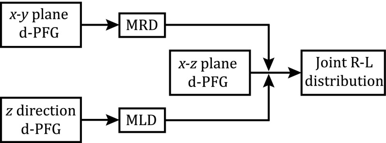
Instead, we suggest applying the concept of separation of variables in an experimental way by a two-step experiment, first independently finding the marginal radius and length distributions and then estimating their joint distribution. The first step involves preforming a set of d-PFG experiments with gradients encoding the orthogonal perpendicular and parallel directions of the cylinder. Both marginal radius and length distributions can be estimated only if the diffusion encoding occurs exclusively in the perpendicular and parallel directions, respectively. Then, to estimate the joint distribution, a d-PFG experiment set with gradients encoding the x-z plane is performed, thus correlating the two orthogonal axes. The marginal radius and length distributions are then used as equality constraints for the estimation of the joint distribution. This pipeline is depicted schematically in Fig. 2.

FIG. 2.

A block diagram of the experimental and analytical framework. The marginal distributions (MRD, MLD) are used to estimate the joint distribution.

A. Marginal radius distribution

The use of gradients that encode the x-y plane by varying the azimuthal angle, φ, between the two PFG pairs, enables the MRD to be estimated, while avoiding molecular displacement information from the parallel direction (Fig. 1(b)). Therefore, in this case, the length of the capped cylinder does not affect the signal attenuation, and the 3D transfer matrix E^xy(Ω, R, L) is naturally reduced to a 2D matrix, since L is degenerate

$${\mathbf{E}}^{xy}(\Omega ,R,L)={\mathbf{E}}^{xy}(\Omega ,R),$$ (5)

and Eq. (1) turns into

$$E^{data}\left({\Omega }_k\right)=\sum _i\Psi \left(R_i\right){\mathbf{E}}^{xy}({\Omega }_k,R_i).$$ (6)

Ψ(R) can then be estimated from

$$E^{data}\left(\Omega \right)={\mathbf{E}}^{xy}(\Omega ,R)\Psi \left(R\right),$$ (7)

by solving Eq. (3).

B. Marginal length distribution

In the case of the MLD, to avoid any x-y component in the acquired signal, the relative angle between the PFG pairs cannot be varied and both pairs have to point to the z direction. Using a s-PFG experiment in the z direction might be possible but would lead to only one experimental variable, G. The disadvantages of using a 1D acquisition in the context of pore size distribution estimation were previously studied and discussed.^33,34 In addition to the extended information resulting from a 2D acquisition, the s-PFG experiment has a lower number of maximal acquired data points, since the minimal step size of G is limited by hardware. Instead, we suggest a novel d-PFG acquisition with both PFG pairs applied over the parallel direction, where |G₁| = G and |G₂| = Gcos (τ); this acquisition would lead to two experimental variables, G and τ, as shown in Fig. 1(c). The values for |G₂| were chosen according to a cosine since it is the projection of the parallel (to the cylinder's symmetry axis) component of an arbitrary gradient on the x-z plane.

When this sequence is used, the radius of the capped cylinder does not affect the signal attenuation, and the 3D transfer matrix E^zz(Ω, R, L) is naturally reduced to a two-dimensional matrix, since R is degenerate

$${\mathbf{E}}^{zz}(\Omega ,R,L)={\mathbf{E}}^{zz}(\Omega ,L),$$ (8)

and Eq. (1) turns into

$$E^{data}\left({\Omega }_k\right)=\sum _i\Psi \left(L_i\right){\mathbf{E}}^{zz}({\Omega }_k,L_i).$$ (9)

Ψ(L) can then be estimated from

$$E^{data}\left(\Omega \right)={\mathbf{E}}^{zz}(\Omega ,L)\Psi \left(L\right),$$ (10)

by solving Eq. (3).

C. Joint radius-length distribution

Before continuing with the strategy to obtain the joint distribution, it is important to recognize the two possible cases in a bivariate distribution. The cylinder radius and length can be either statistically independent or dependent. If R and L are independent variables, their joint probability can be expressed as

$$\mathit{\Psi }(R,L)=\Psi \left(R\right){\Psi \left(L\right)}^T,$$ (11)

and since both marginal probabilities have been already found, estimating $\mathit{\Psi }(R,L)$ becomes trivial.

But for the general case, a dependency may exist between R and L. To obtain information that correlates the two orthogonal axes, parallel and perpendicular, we suggest using a d-PFG experiment with gradient directions that vary in the x-z plane, as shown in Fig. 1(d). Since in each measurement both the perpendicular and parallel axes of the capped cylinder are being encoded, we can no longer ignore one of the cylinder's dimensions. It follows that the transfer matrix is indeed 3D. Furthermore, the probability density function now depends on both R and L, and is in fact the joint distribution, $\mathit{\Psi }(R,L)$. In this case, Eq. (1) can be written as

$$E^{xz}\left({\Omega }_k\right)=\sum _i\sum _j\mathit{\Psi }(R_i,L_j){\mathbf{E}}^{xz}({\Omega }_k,R_i,L_j),$$ (12)

where ∑_i∑_jΨ (R_i, L_j) = 1.

As suggested earlier, to solve Eq. (12), the matrix $\mathit{\Psi }(R,L)$ has to be written as a vector. Instead of the two variables, R and L, we shall define Λ = (R, L), which is a combination of a specific R, L couple. Therefore, a system of N radii and M lengths should have N · M (R, L) couples, Λ. Equation (12) is then reduced to

$$E^{xz}\left({\Omega }_k\right)=\sum _p\Psi \left({\Lambda }_p\right){\mathbf{E}}^{xz}({\Omega }_k,{\Lambda }_p),$$ (13)

where ∑_pΨ(Λ_p) = 1.

Because the number of coefficients that must be estimated here is N · M, which is normally large, the large amount of acquired data that are required soon becomes infeasible. Adding equality constraints to Eq. (3) stabilizes the inversion by limiting and narrowing the solution space of the least square minimization. This vital process can be achieved since we have obtained the two marginal distributions, Ψ(R) and Ψ(L), which are related to the joint distribution as

$$\begin{array}{c}\hfill \sum _j\mathit{\Psi }(R,L_j)=\Psi \left(R\right)\mathrm{and}\sum _i\mathit{\Psi }(R_i,L)=\Psi \left(L\right).\end{array}$$ (14)

Applying the equality constraints in Eq. (14) while solving the minimization problem in Eq. (3), leads to a stable nonparametric estimation of the joint radius-length distribution. Thanks to these constraints, the system is allowed to be underdetermined (i.e., more variables than equations) and yet solvable.

The importance of CSA was discussed in the Introduction. The current framework allows a direct measurement of the anisotropy variation within the sample in the form of cylinder eccentricity distribution. If we follow Özarslan's definition of the finite cylinder's eccentricity, ε = L/(2R),²⁰ then the eccentricity probability distribution, Ψ(ε) can be determined from $\mathit{\Psi }(R,L)$. After defining an eccentricity matrix $\mathtt{E}(R_i,L_j)=L_j/\left(2R_i\right)$, the probability of each element from the corresponding joint distribution matrix can be appropriately assigned.

III. METHODS

A. Experimental parameters

The current framework requires d-PFG experiments performed in both the z axis and the x-y and x-z planes aligned with the principal axes of the capped cylinders, as discussed in Sec. II and as illustrated in Fig. 1. In this case, it is easier to describe the gradient wave vectors within a spherical coordinate system, as defined in Fig. 1(a) (top). Each gradient vector is defined by its amplitude; azimuthal angle, φ; and polar angle, θ.

For the purpose of this study, the different experimental parameter sets, Ω, differed only by three parameters, Δ, G, and the relevant angle (φ, θ, and τ in the case of the x-y plane, x-z plane, and z direction, respectively). This methodology creates a 3D parametric space for diffusion encoding. The remaining experimental parameters, namely, δ = 3 ms and t_m = 0, were fixed. In addition, the diffusion coefficient was set to be D = 1.8 μm²/ms. Since the wave vector q = (2π)⁻¹γδG (γ is the gyromagnetic ratio of the labeled spins) reflects the diffusion weighting and provides direct insight to the physical dimension of the pore, we will use it instead of G.

Although infinite possible experimental sets, Ω, exist, a judicious choice of specific experimental parameters improves the size distribution reconstruction.³³ In the present study, we have followed a version of a previously suggested optimization framework.³⁴ This iterative method is designed to select experimental data sets that balance the need to lower the inherent ill posedness and increase the MR signal intensity. It is suggested that no single metric of the transfer matrix (e.g., column rank) can be used to predict the quality of the estimation. Instead, the stability of the inversion is related to the transfer matrix column rank, condition number, and signal-to-noise ratio (SNR). In the present work, the selection of the optimal experimental sets was done in two iterative steps. First, an experimental parameters set that results in a full rank transfer matrix is determined; then this set is used as an initial guess while a search is carried out to find the experimental set that minimizes the transfer matrix condition number. A detailed description of the algorithm is provided elsewhere.³⁴

The dimensions of the capped cylinders were assumed to lie within the range of axonal tissue. In this case, the nominal size in the parallel axis of the cylinder is expected to be larger than that in the perpendicular axis, therefore directly affecting the signal attenuation profiles and leading to generally stronger attenuation in the z direction. This discrepancy requires the application of weaker gradients in the z and x-z experiments. For the estimation of the marginal distributions, we have found that about ten times more equations than free parameters are needed, a finding which is consistent with previous publications.³⁴

1. x-y plane

In the x-y plane d-PFG experiment, the direction of |q₁| = q was (φ, θ) = (0, π/2), while the direction of |q₂| = q was varied in the x-y plane, such that (φ, θ) = (0 − π, π/2) (Fig. 1(b)).

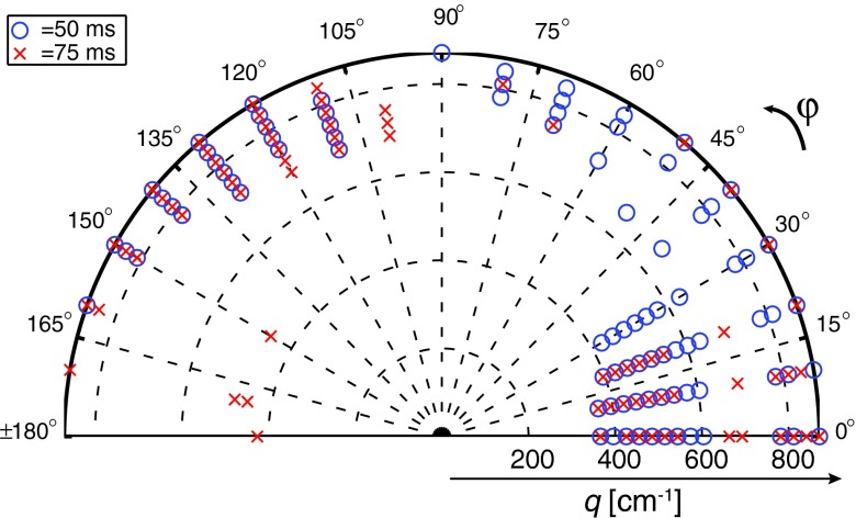
The transfer matrix, E^xy(Ω, R), was generated with a cylinder radius range of 0.6 μm ⩽ R ⩽ 10 μm with 0.6 μm steps; this range led to 16 different pore radii. Upon optimization, 160 different experimental sets were chosen from the 3D parametric space created by φ = 0 − π, q = 366 − 871 cm⁻¹, and Δ = 50, 75 ms. As an example, the optimized experimental sets used in the x-y plane d-PFG are shown in Fig. 3.

FIG. 3.

The optimized x-y plane acquisition scheme that includes 160 data sets from the 3D parametric space spanned by q, φ, and Δ.

2. z direction

In the z direction d-PFG experiment, the direction of both |q₁| = q and |q₂| = qcos (τ) was (φ, θ) = (0, 0), while q₂ was varied according to τ.

The transfer matrix, E^zz(Ω, L), was generated with a cylinder length range of 5 μm ⩽ L ⩽ 40 μm, with 1.4 μm steps; this range led to 26 different pore lengths. Upon optimization, 240 different experimental sets were chosen from the 3D parametric space created by τ = 0 − π, q = 60 − 594 cm⁻¹, and Δ = 50, 75 ms.

3. x-z plane

Two versions were used in the x-z plane d-PFG experiment: (1) the direction of |q₁| = q was (φ, θ) = (0, 0), while the direction of |q₂| = q was varied in the x-z plane, such that (φ, θ) = (0, 0 − π); (2) the direction of |q₁| = q was (φ, θ) = (0, π/2), while the direction of |q₂| = q was varied in the x-z plane, such that (φ, θ) = (0, π/2 − 3π/2).

The transfer matrix, E^xz(Ω, R, L), was generated with the same R and L steps used to generate E^xy(Ω, R), and E^zz(Ω, L), respectively, which led to 416 different (R, L) combinations. Upon optimization, 150 different experimental sets were chosen from the 3D parametric space created by θ = 0 − 3π/2, q = 59 − 623 cm⁻¹, and Δ = 50, 75 ms.

The typical diffusion length, $L_D=\sqrt{2D\Delta }=16.4\mu \text{m}$, is shorter than the maximal considered length (40 μm). Representing the mean displacement of free diffusing molecules, L_D should not be used as the maximal restricting dimension, since this assumption implicitly suggests that for a compartment with L > L_D, all molecules experience Gaussian diffusion. However, while the mean displacement of the ensemble of spins is known, the spins are uniformly distributed within the compartment, and so are their initial positions. When the first diffusion gradient is applied, spins that are close to the compartment boundary do experience restriction, and they are responsible for the deviation from Gaussian diffusion even when L ≫ L_D. A simulation that demonstrates this deviation is provided in the Appendix.

4. Inversion details

All implementations of the theory were performed with Matlab^® (R2013a, The MathWorks, Natick, MA) in-house algorithms. To form the transfer matrix, all of the signal attenuation curves were generated with the multiple correlation function (MCF) method,³⁷ which was later extended to describe d-PFG MR experiments.³⁸ The capped cylinder geometry considered in this article is envisioned as a combination of two parallel plates and a cylinder whose symmetry axis is oriented along the z-direction (Fig. 1), as previously proposed.²⁰ The partial volumetric fraction vector, Ψ, was then obtained by implementing a non-negative least-square algorithm with an added constraint, that ∑_iΨ_i = 1 (and for the joint distribution, the additional equality constraint in Eq. (14)), using the lsqlin Matlab function. Note that no regularization was used in the fitting process. For the moment, we avoid using regularization methods since they are problem specific, and the selection of the regularization parameter may affect the results.

Because of the equality constraints, the reconstruction of the joint distribution was possible with fewer equations than variables, namely, 150 and 416, respectively. The stability of this underdetermined system results in a relatively low number of acquisitions and thus a feasible experimental design.

Throughout the study the estimation quality was assessed based on the Jensen difference³⁹ between the theoretical and estimated PSDs. The Jensen difference metric is a symmetric version of the Kullback-Leibler divergence, but it always yields a finite value. The difference between two PSDs, Q and P, is defined as⁴⁰

$$\begin{array}{ccc}\hfill d_{JD}& =& \sum _i[\frac{P_i\ln \left(P_i\right)+Q_i\ln \left(Q_i\right)}{2}\hfill \\ & & -\left(\frac{P_i+Q_i}{2}\right)\ln \left(\frac{P_i+Q_i}{2}\right)].\hfill \end{array}$$ (15)

The Jensen difference metric was chosen since it is a well-established method of measuring the similarity between two probability distributions.

B. Simulated joint distribution phantoms

In the case of axon bundles, there are pore size distributions that appear to be lognormal or multimodel, as in many distributions occurring in nature and granular media.⁴ This notion had led us to use a weighted linear combination of bivariate lognormal distribution functions to form two joint R-L distribution phantoms (Figures 4(a) and 4(b)). In addition, a more general R-L distribution was considered (Fig. 4(c)) to demonstrate the power of the presented approach. While this distribution is clearly not realistic, its marginal radius and length distributions have very few non-negative coefficients, thus making the estimation process more challenging.

FIG. 4.

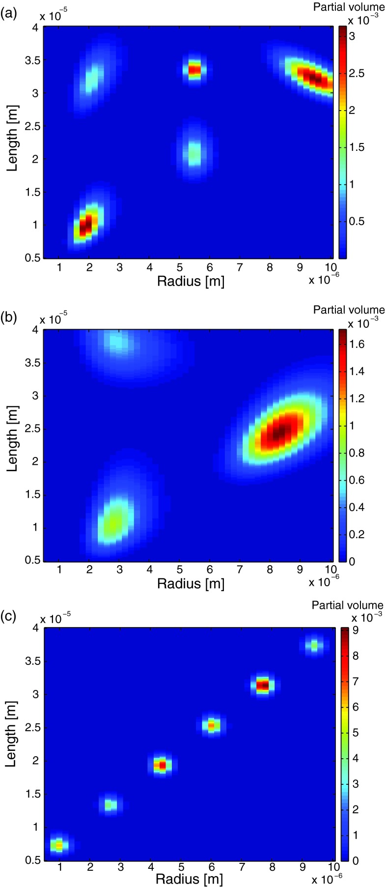
Joint R-L distribution phantoms representing two realistic cases of microstructure: (a) five narrow peaks (referred to as “dense-narrow”) and (b) three broad peaks (referred to as “scattered-broad”) in the R-L space, while in (c), a more general and demanding distribution is considered (referred to as “random-diagonal”).

The general form of the lognormal probability density function was

$$\begin{array}{ccc}\hfill f(R,L)& =& \frac{1}{2\pi RL{\tilde{\sigma }}_R{\tilde{\sigma }}_L\sqrt{1-{\rho }^2}}\left(\exp \right[-\frac{1}{2(1-{\rho }^2)}\hfill \\ \hfill & & \times [{\left(\frac{\log \left(R\right)-{\tilde{R}}_0}{{\tilde{\sigma }}_R}\right)}^2-2\rho \left(\frac{\log \left(R\right)-{\tilde{R}}_0}{{\tilde{\sigma }}_R}\right)\hfill \\ \hfill & & \times \left(\frac{\log \left(L\right)-{\tilde{L}}_0}{{\tilde{\sigma }}_L}\right)+{\left(\frac{\log (L-{\tilde{L}}_0}{{\tilde{\sigma }}_L}\right)}^2\left]\right]),\hfill \end{array}$$ (16)

where

$$\begin{array}{cc}\hfill {\tilde{\sigma }}_x& ={\left[\log \left(1+\frac{{\sigma }_x^2}{x_0^2}\right)\right]}^{\frac{1}{2}},\hfill \\ \hfill {\tilde{x}}_0& =\log \left(x_0\right)-\left(\frac{{\tilde{\sigma }}_x^2}{2}\right).\hfill \end{array}$$

x₀ and σ_x are the mean and standard deviation of either R or L, and ρ is the correlation coefficient of log (R) and log (L).

The following three joint R-L distribution phantoms were simulated:

• 1.Dense-narrow peak distribution: Five bivariate lognormal probability density functions, as shown in Fig. 4(a), with the following parameters: centers (all in μm) (R₀, L₀) = (2.0, 10.4), (2.2, 32.4), (9.5, 32.2), (5.5, 21.0), (5.5, 33.5); standard deviations (all in μm) (σ_R, σ_L) = (0.25, 1.5), (0.30, 2.0), (0.40, 1.1), (0.30, 2.0), (0.20, 1.0); correlation coefficients ρ = (0.5, 0.5, −0.7, 0, 0); and relative fractions 0.25, 0.15, 0.25, 0.2, 0.15.
• 2.Scattered-broad peak distribution: Three broad bivariate lognormal probability density functions, as shown in Fig. 4(b), with the following parameters: centers (all in μm) (R₀, L₀) = (3.0, 12.0), (3.2, 38.4), (8.5, 25.2); standard deviations (all in μm) (σ_R, σ_L) = (0.50, 3.0), (0.80, 3.0), (0.65, 2.5); correlation coefficients ρ = (0.35, −0.25, 0.55); and relative fractions 0.25, 0.25, 0.50.
• 3.Random-diagonal peak distribution: Six narrow bivariate lognormal probability density functions, as shown in Fig. 4(c), with the following parameters: centers (all in μm) (R₀, L₀) = (1.0, 7.4), (2.7, 13.4), (4.4, 19.4), (6.0, 25.4), (7.7, 31.4), (9.4, 37.4); all with the same standard deviations (in μm) (σ_R, σ_L) = (0.20, 0.8) and correlation coefficients ρ = 0; the relative fractions were randomly generated and were 0.15, 0.11, 0.21, 0.17, 0.25, 0.11.

To approach the continuous nature of an actual size distribution, the signal attenuation profile, E^data(Ω), was generated using an appropriate transfer matrix with very fine, equal-sized spatial steps of 0.2 μm in both R and L. In addition, all of the generated signal curves were corrupted by Gaussian white noise. For each distribution, two noise standard deviations were analyzed, namely, 0.5% and 1% relative to the signal attenuation without any diffusion gradient applied.

IV. RESULTS

The joint R-L distribution of capped cylinders was estimated after following the steps described schematically in Fig. 2. Three joint distributions were simulated (Fig. 4), accounting for different peak widths and separations.

A. Advantage of constraints

First, it is important to provide clear evidence that the use of the marginal radius and length distributions as equality constraints in the joint distribution estimation improves the results. To this end, the estimation of the joint distribution was performed without using the marginal distributions. Furthermore, a fair comparison would have to include in the estimation process all of the data points from the x-y plane and the z direction, along with the x-z plane acquisition originally proposed to estimate the joint distribution.

Because the underlying data sets of the marginal distributions are included, the transfer matrix becomes overdetermined (all 160, 240, and 150 experimental sets from the x-y plane, z direction, and x-z plane, respectively).

The dense-narrow peak distribution phantom with a noise standard deviation of 0.5% was used for the comparison. This particular phantom was selected since it represents the “easiest” case for estimation because of the relatively small number of non-zero elements, and the low noise level.

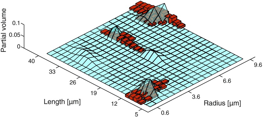
In Fig. 5, the theoretical joint distribution (solid surface) and the estimated one (bins) are shown after the minimization problem in Eq. (3) has been solved without the equality constraints. Fig. 5 should be compared to Fig. 8(a).

FIG. 5.

The theoretical (solid surface) and estimated (bins) joint R-L distribution of the dense-narrow peak distribution phantom with a noise standard deviation of 0.5%, without the use of the equality constraints.

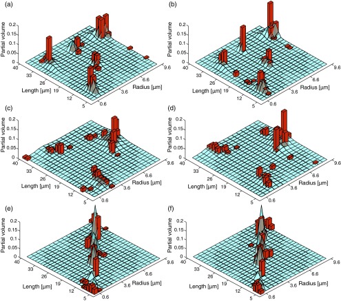
FIG. 8.

The theoretical (solid surface) and estimated (bins) joint R-L distributions of all of the phantoms. Dense-narrow distribution with noise standard deviations of (a) 0.5% and (b) 1%. Scattered-broad distribution with noise standard deviations of (c) 0.5% and (d) 1%. Random-diagonal distribution with noise standard deviations of (e) 0.5% and (f) 1%.

B. Estimation of marginal and joint distributions

As described above, the MRD was estimated from an x-y plane d-PFG experiment. In Fig. 6, the theoretical MRDs of all of the phantoms were drawn as a function of the radius (solid line), while the estimated MRDs were overlaid on it (bins). The MRDs of the narrow peak distribution in Fig. 4(a), presented in Figures 6(a) and 6(d), correspond to noise standard deviations of 0.5% and 1%, with Jensen differences of 0.0393 and 0.0431, respectively. The MRDs of the broad peak distribution in Fig. 4(b), presented in Figures 6(b) and 6(e), correspond to noise standard deviations of 0.5% and 1%, with Jensen differences of 0.0653 and 0.1032, respectively. Finally, the MRDs of the random-diagonal peak distribution in Fig. 4(c), presented in Figures 6(c) and 6(f), correspond to noise standard deviations of 0.5% and 1%, with Jensen differences of 0.0764 and 0.0867, respectively.

FIG. 6.

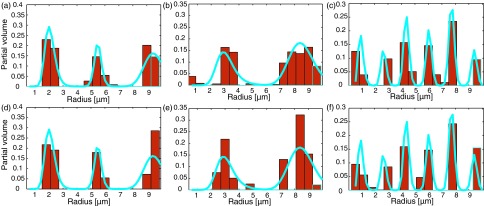
The theoretical (solid line) and estimated (bins) MRDs of all of the phantoms. Dense-narrow distribution with noise standard deviations of (a) 0.5% and (d) 1%. Scattered-broad distribution with noise standard deviations of (b) 0.5% and (e) 1%. Random-diagonal distribution with noise standard deviations of (c) 0.5% and (f) 1%.

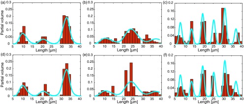
Next, the MLD was estimated from a z-direction d-PFG experiment. In Fig. 7, the theoretical MLDs of all of the phantoms were drawn as a function of the radius (solid line), while the estimated MLDs were overlaid on it (bins). The MLDs of the narrow peak distribution (Fig. 4(a)) are presented in Figures 7(a) and 7(d); they correspond to noise standard deviations of 0.5% and 1%, with Jensen differences of 0.0524 and 0.0807, respectively. The MLDs of the broad peak distribution in Fig. 4(b), presented in Figures 7(b) and 7(e), correspond to noise standard deviations of 0.5% and 1%, with a Jensen differences of 0.0480 and 0.1185, respectively. Finally, the MLDs of the random-diagonal peak distribution in Fig. 4(c), presented in Figures 7(c) and 7(f), correspond to noise standard deviations of 0.5% and 1%, with Jensen differences of 0.1131 and 0.1197, respectively.

FIG. 7.

The theoretical (solid line) and estimated (bins) MLDs of all of the phantoms. Dense-narrow distribution with noise standard deviations of (a) 0.5% and (d) 1%. Scattered-broad distribution with noise standard deviations of (b) 0.5% and (e) 1%. Random-diagonal distribution with noise standard deviations of (c) 0.5% and (f) 1%.

Unless the radii and lengths of the ensemble of cylinders are statistically independent, the marginal distributions provide only a fragment of the microstructural information. An x-z plane d-PFG experiment should be used to obtain the full description from the joint R-L distribution. In Fig. 8, the theoretical (solid surface) joint distributions of all of the phantoms and the estimated ones (bins) are shown. The narrow peak R-L distributions are presented in Figures 8(a) and 8(b); they correspond to noise standard deviations of 0.5% and 1%, with Jensen differences of 0.2703 and 0.2774, respectively. The broad peak distributions presented in Figures 8(c) and 8(d), correspond to noise standard deviations of 0.5% and 1%, with Jensen differences of 0.3407 and 0.3464, respectively. Finally, the random-diagonal peak distributions presented in Figures 8(e) and 8(f), correspond to noise standard deviations of 0.5% and 1%, with Jensen differences of 0.2343 and 0.2184, respectively.

The influence of added noise can be seen by following the changes in the Jensen differences. For the MRDs, the SNR decrease resulted in a Jensen difference increase of 10%, 58%, and 13%, for the narrow, broad, and diagonal peak distributions, respectively. For the MLDs, the SNR decrease resulted in a Jensen difference increase of 54%, 147%, and 6%, for the narrow, broad, and diagonal peak distributions, respectively. Interestingly, for the joint distributions, the SNR decrease resulted in a Jensen difference increase of only 2.6% and 1.7% for the narrow and broad distributions, respectively, and a 6.8% decrease for the diagonal peak distribution.

V. DISCUSSION

We have presented an experimental design and analytical framework to estimate the nonparametric joint radius-length distribution of an ensemble of capped cylinders. The major innovations are the use of a 3D d-PFG MR acquisition to obtain the marginal radius and length distributions and then employing these as equality constraints in the estimation of the joint R-L distribution. The suggested framework exploits the ability to acquire the MR signal from orthogonal cross sections of the pore by selectively applying the diffusion gradients along different directions. The 3D d-PFG experiment can be decomposed into three steps. First, the direction of the diffusion gradients is kept in the x-y plane, allowing us to estimate the MRD by treating the capped cylinder as an infinite one. Second, the d-PFG gradient pairs are applied along the z axis, so that the MLD is estimated by treating the capped cylinders as parallel plates. The final step involves applying gradients in the x-z plane, which results in MR signal attenuation that is influenced by the distribution of both pore length and radius. Although there are many coefficients to estimate in the joint R-L distribution, a relatively small number of acquisitions is needed to reconstruct it. In fact, the transfer matrix that is used to obtain the joint distribution can be underdetermined, thanks to the use of the previously estimated MRD and MRL as equality constraints.

Three joint R-L distribution phantoms, exhibiting a range of pore morphologies, were used to demonstrate the versatility of the proposed framework. The first two cases represented realistic scenarios for axonal morphology, and contained joint distributions with five narrow peaks (referred to as “dense-narrow”) and three broad peaks (referred to as “scattered-broad”) in the R-L parameter space. The third phantom (referred to as “random-diagonal”) contained a more general R-L distribution in an attempt to establish the power of the presented approach. In all cases, the MRDs, MLDs, and joint R-L distribution were estimated subject to different noise (SNR) levels (σ = 0.005, 0.01).

Estimation without constraints was performed to determine that using the marginal radius and length distributions as equality constraints in the joint distribution estimation indeed improves the results. The dense-narrow distribution with σ = 0.005 case was used as a phantom because of the relatively small number of non-zero elements and the low noise level. This step was done without the use of the marginal distributions as equality constraints but did include all 160, 240, and 150 experimental sets from the x-y plane, z direction, and x-z plane, respectively. The resulting joint distribution reconstruction is clearly inaccurate, as two out of the five peaks are missing, and the rest of the estimated peaks are much broader than predicted (Fig. 5).

In contrast, when using the equality constraints, the reconstruction of the dense-narrow peaks proved fairly stable to noise level increases for both the marginal and joint distributions. This stability can be seen qualitatively from Figures 6–8, and quantitatively from the minor changes in the Jensen difference (a 10%, 54%, and 2.6% change for the MRD, MLD, and joint, respectively) due to decreases in the SNR.

With the exception of the joint distribution estimation, the reconstructions of the scattered-broad peak distributions were sensitive to decreasing SNR, for both marginal distributions. Generally, as the size distribution becomes broader, including a greater number of non-zero values, reconstruction of the peak distribution becomes less stable. Therefore, large standard deviations that result in wider peaks along with low SNR should be expected to yield estimates with lower accuracy. Even though the Jensen difference increased by 58% and 147% for the MRD and MLD, respectively, it only increased by 1.7% for the joint distribution.

The random-diagonal phantom provided a test case in which both of the marginal distributions always have more non-zero than zero elements, with a random value amplitude. This case also proved fairly stable to noise level increases as can be seen from the minor changes in the Jensen difference (a 13%, 6%, and 6.8% change for the MRD, MLD, and joint distribution, respectively) due to decreases in the SNR.

One of the advantages of using the marginal distributions as equality constraints is that they reduce the number of unknown parameters in the joint distribution. It is therefore important to look at the number of non-negative elements found during estimation of the marginal distributions, since they will later determine the remaining unknown parameters in the joint distribution estimation process. For the dense-narrow peaks, the marginal distributions reveal that there are about 8 and 13 non-zero radii and lengths, respectively. With these as equality constraints, there are 104 remaining unknowns for the joint distribution, effectively making the system overdetermined (the x-z experiment had 150 data sets). This is not the case for the scattered-broad and random-diagonal distributions, for which there are 276 and 230 remaining unknowns, respectively, making the system underdetermined. The robustness of the joint R-L distribution to noise level and standard deviation is remarkable since the estimation is performed with what is potentially a very underdetermined system (416 partial volume elements).

The ranges of radii and lengths within the joint distribution phantoms were based on beaded axonal morphologies, and the expected ranges of these values such a specimen may contain.⁸ Little information regarding the shape of the joint distribution of beaded axons is currently available; therefore there is no basis or a priori information to impose for assuming a particular parametric size or shape distribution. Furthermore, it is reasonable to posit that severity of the injury may affect the form of the joint R-L distribution; therefore, assuming a specific parametric distribution is not warranted. All of the estimated marginal and joint distributions are nonparametric, and, therefore, not based on any assumed pore size or eccentricity.

As previously shown,^33,34 a judicious choice of specific experimental parameters, and/or increased dimensionality of the parametric space (by varying other new salient parameters, e.g., δ) can improve the stability of the size distribution estimation. For the purpose of introducing the current framework, a d-PFG 3D parameter space of independent experimental variables was assumed, from which the values of q, φ/θ/τ, and Δ were selected according to an optimization scheme described in Sec. III. The optimized data point sets from the x-y plane d-PFG experiment are shown in Fig. 3. Other experimental design optimization schema can be incorporated into the joint radius-length distribution estimation framework, as an additional preliminary step.

It has been previously shown⁴¹ that a s-PFG experiment with a varying diffusion period is equivalent to a d-PFG experiment to the second moment of the total signal decay. While an important observation, the d-PFG experiment is preferable for the purpose of resolving the PSD. The d-PFG experiment is uniquely suited to pore size and shape characterization. The ability to perform the d-PFG experiment in a chosen physical plane is a key element that enables the estimation of the joint radius-length distribution. In addition, the theoretical advantages of the d-PFG over the s-PFG experiment in the context of the pore size distribution estimation problem were previously shown and discussed,^33,34 and later experimentally demonstrated.⁴² The application of two PFG pairs (i.e., d-PFG) as opposed to one (i.e., s-PFG) results in a higher sensitivity to different pore sizes, making the solution to this inverse problem less ill posed. Moreover, use of the d-PFG experiment leads to more and new information, increasing the dimensionality of the column space of the transfer matrix, making the estimation more robust.

The underlying assumption behind the present method is that when it is used in neural tissue, specifically white matter, axons are coherently oriented finite cylinders. In the case of brain white matter tissue, fascicles containing axons are expected to take on all possible orientations within an imaging volume. Two general cases of cylinder orientation can be envisioned, namely, parallel cylinders of unknown direction and randomly oriented cylinders. A preliminary diffusion tensor imaging (DTI) scan⁴³ can be used to identify the case in hand. The amount of anisotropy resulting from the DTI experiment is related to the orientation coherence within a voxel, as randomly oriented cylinders would appear to be isotropic. After identifying and establishing the suitable orientation description, we suggest two experimental and analytical strategies to address the problem.

If the cylinders are found to be parallel with a varying orientation over different voxels, an adjustment to the experimental design is necessary. Komlosh et al.⁴⁴ used a 3D gradient sampling scheme that involves the application of the current circular d-PFG acquisition in different orientations, similar to the design of DTI experiments. The principal fiber orientation in each voxel can then be calculated from a subset of these measurements (or from the previous DTI scan), and the projection of the data onto the desired plane can be used and analyzed. Although costly in experimental time, this strategy is especially well suited for the joint distribution estimation framework, since a 3D d-PFG acquisition is already being used.

If the cylinders are found to be randomly oriented, one can use the current experimental framework and address the orientation distribution with a slight analytical addition. A uniform orientation distribution (i.e., random orientation) of cylinders can be assumed,²⁰ thus modifying the calculation of the signal attenuation constructing the transfer matrix. Evidently, the isotropic nature of the macrostructure would eliminate the possibly of decoupling R and L, and obtaining the marginal distributions. A more complicated orientation distribution (i.e., not random) would require additional free parameters and is out of the scope of this work.

The determination of the joint radius-length distribution permits direct quantification of the CSA. This framework was introduced using the capped cylinder geometry, but can be implemented for any anisotropic pore shape that is solvable with the MCF method (e.g., ellipsoids with different major and minor axes). Measuring the CSA of injured (beaded) axons may help to characterize and quantify the amount of damage to the tissue and shed light on the injury mechanism and the possible microstructural changes that may occur following the injury. To adapt the model to real nervous tissue, additional components can be added to the current capped cylinders, such as a distribution of infinite cylinders, representing healthy axons, and a Gaussian extracellular diffusion compartment. Such a model may provide vital information about changes following injury, or even during development.

Diffusion weighed MR techniques have already been used to determine skeletal muscle architecture.^45–47 The length and cross-sectional area of myocytes are structural features that are proportional to muscle force and velocity that can be directly obtained from a joint radius-length distribution. Following changes in the joint distribution may help to explain the way that muscle tissue responds to freezing and thawing alternations in food sciences applications or help explain and improve tissue preservation in transplantation applications. The presented framework may also be used to directly measure noninvasively the CSA of sieve tube elements, thus shedding light on nutrient translocation within plants.

APPENDIX: MAXIMAL CYLINDER SIZE

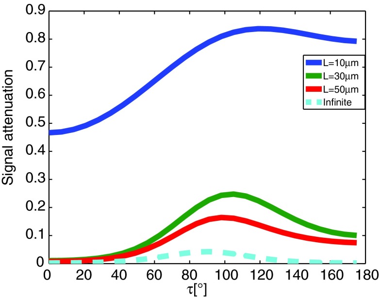
It is important to discuss the validity of the selected range of radii and lengths in this work (0.6 μm − 10 μm and 5 μm − 40 μm, respectively). The relevant experimental parameters, namely, Δ_min = 50 ms and D = 1.8 μm²/ms, determine the largest mean ensemble displacement according to $L_D=\sqrt{2D\Delta }=16.4\mu \text{m}$. It was previously suggested³⁰ that the product of the Einstein diffusion formula be used as the maximal restricted dimension. This assumption implicitly suggests that for any larger restricted dimension, water molecules experience Gaussian (i.e., free) diffusion. In our case, if one adopts this suggestion, the upper boundary of the possible cylinder radii and lengths has to be 16.4 μm or lower. The MCF signal calculation framework, which is capable of handling arbitrary experimental parameters, can be used to check the validity of this upper boundary.

A d-PFG z-direction experiment using the current study's experimental parameters and q = 300 cm⁻¹ was simulated, both with capped- and infinite-cylinder geometries. In the capped-cylinder case, three representative lengths were chosen, while all but one were subject to L > L_D. It is clear from the simulation results (Fig. 9) that even though the length of the cylinder considerably and excessively violates L_D, the signal attenuation curves do not resemble those that result from freely diffusing spins in the cylinder's parallel axis. It is therefore incorrect to assume Gaussian diffusion along the restricted direction. It is clear that the use of L_max = 40 μm in our case is valid.

FIG. 9.

Signal attenuation from capped (solid lines) and infinite cylinders (dashed line). Three different lengths of finite cylinders are presented, where all but one is subject to L > L_D.

REFERENCES

- 1.Katchalsky A. K. and Curran P. F., Nonequilibrium Thermodynamics in Biophysics (Harvard University Press, Cambridge, 1965). [Google Scholar]
- 2.Tasaki I., Ishii K., and Ito H., “On the relation between the conduction-rate, the fiber-diameter and the internodal distance of the medullated nerve fiber,” Jpn. J. Med. Sci. III, Biophys. 9, 189–199 (1943). [Google Scholar]
- 3.Waxman S., Kocsis J., and Stys P., The Axon: Structure, Function, and Pathophysiology (Oxford University Press, New York, 1995). [Google Scholar]
- 4.Pajevic S. and Basser P. J., “An optimum principle predicts the distribution of axon diameters in normal white matter,” PloS One 8, e54095 (2013). 10.1371/journal.pone.0054095 [DOI] [PMC free article] [PubMed] [Google Scholar]
- 5.Ochs S. and Jersild R. A., “Cytoskeletal organelles and myelin structure of beaded nerve fibers,” Neuroscience 22, 1041–1056 (1987). 10.1016/0306-4522(87)92979-4 [DOI] [PubMed] [Google Scholar]
- 6.Ochs S., Pourmand R., Jersild R. A., and Friedman R. N., “The origin and nature of beading: A reversible transformation of the shape of nerve fibers” Prog. Neurobiol. 52, 391–426 (1997). 10.1016/S0301-0082(97)00022-1 [DOI] [PubMed] [Google Scholar]
- 7.Roediger B. and Armati P. J., “Oxidative stress induces axonal beading in cultured human brain tissue,” Neurobiol. Dis. 13, 222–229 (2003). 10.1016/S0969-9961(03)00038-X [DOI] [PubMed] [Google Scholar]
- 8.Budde M. D. and Frank J. A., “Neurite beading is sufficient to decrease the apparent diffusion coefficient after ischemic stroke” Proc. Natl. Acad. Sci. U.S.A. 107, 14472–14477 (2010). 10.1073/pnas.1004841107 [DOI] [PMC free article] [PubMed] [Google Scholar]
- 9.Magid A. and Law D. J., “Myofibrils bear most of the resting tension in frog skeletal muscle” Science 230, 1280–1282 (1985). 10.1126/science.4071053 [DOI] [PubMed] [Google Scholar]
- 10.Hanft L. M. and McDonald K. S., “Length dependence of force generation exhibit similarities between rat cardiac myocytes and skeletal muscle fibres,” J. Physiol. 588, 2891–2903 (2010). 10.1113/jphysiol.2010.190504 [DOI] [PMC free article] [PubMed] [Google Scholar]
- 11.Martin R. B., “Porosity and specific surface of bone,” Crit. Rev. Biomed. Eng. 10, 179–222 (1984). [PubMed] [Google Scholar]
- 12.Currey J. D., “The effect of porosity and mineral content on the Young's modulus of elasticity of compact bone,” J. Biomech. 21, 131–139 (1988). 10.1016/0021-9290(88)90006-1 [DOI] [PubMed] [Google Scholar]
- 13.Yeni Y. N. and Norman T. L., “Fracture toughness of human femoral neck: Effect of microstructure, composition, and age,” Bone 26, 499–504 (2000). 10.1016/S8756-3282(00)00258-1 [DOI] [PubMed] [Google Scholar]
- 14.Wang X. and Ni Q., “Determination of cortical bone porosity and pore size distribution using a low field pulsed NMR approach,” J. Orthop. Res. 21, 312–319 (2003). 10.1016/S0736-0266(02)00157-2 [DOI] [PubMed] [Google Scholar]
- 15.Esau K., The Phloem (Gebruder Borntraeger, Berlin, 1969). [Google Scholar]
- 16.Mullendore D. L., Windt C. W., Van As H., and Knoblauch M., “Sieve tube geometry in relation to phloem flow” Plant cell 22, 579–593 (2010). 10.1105/tpc.109.070094 [DOI] [PMC free article] [PubMed] [Google Scholar]
- 17.Stejskal E. and Tanner J., “Spin diffusion measurements: Spin echoes in the presence of a time-dependent field gradient,” J. Chem. Phys. 42, 288–292 (1965). 10.1063/1.1695690 [DOI] [Google Scholar]
- 18.Callaghan P., Coy A., MacGowan D., Packer K., and Zelaya F., “Diffraction-like effects in NMR diffusion studies of fluids in porous solids,” Nature (London) 351, 467–469 (1991). 10.1038/351467a0 [DOI] [Google Scholar]
- 19.Basser P. J., “Inferring microstructural features and the physiological state of tissues from diffusion-weighted images” NMR Biomed. 8, 333–344 (1995). 10.1002/nbm.1940080707 [DOI] [PubMed] [Google Scholar]
- 20.Ozarslan E., “Compartment shape anisotropy (CSA) revealed by double pulsed field gradient MR,” J. Magn. Reson. 199, 56–67 (2009). 10.1016/j.jmr.2009.04.002 [DOI] [PMC free article] [PubMed] [Google Scholar]
- 21.Cory D., Garroway A., and Miller J., “Applications of spin transport as a probe of local geometry,” Polym. Preprints 31, 149–150 (1990). [Google Scholar]
- 22.Mitra P., “Multiple wave-vector extensions of the NMR pulsed-field-gradient spin-echo diffusion measurement,” Phys. Rev. B 51, 15074–15078 (1995). 10.1103/PhysRevB.51.15074 [DOI] [PubMed] [Google Scholar]
- 23.Stapf S., Damion R., and Packer K., “Time correlations in fluid transport obtained by sequential rephasing gradient pulses” J. Magn. Reson. 137, 316–323 (1999). 10.1006/jmre.1998.1685 [DOI] [PubMed] [Google Scholar]
- 24.Ozarslan E. and Basser P. J., “MR diffusion - “diffraction” phenomenon in multi-pulse-field-gradient experiments,” J. Magn. Reson. 188, 285–294 (2007). 10.1016/j.jmr.2007.08.002 [DOI] [PMC free article] [PubMed] [Google Scholar]
- 25.Koch M. A. and Finsterbusch J., “Compartment size estimation with double wave vector diffusion-weighted imaging,” Magn. Reson. Med. 60, 90–101 (2008). 10.1002/mrm.21514 [DOI] [PubMed] [Google Scholar]
- 26.Komlosh M. E., Özarslan E., Lizak M. J., Horkay F., Schram V., Shemesh N., Cohen Y., and Basser P. J., “Pore diameter mapping using double pulsed-field gradient MRI and its validation using a novel glass capillary array phantom,” J. Magn. Reson. 208, 128–135 (2011). 10.1016/j.jmr.2010.10.014 [DOI] [PMC free article] [PubMed] [Google Scholar]
- 27.Lawrenz M. and Finsterbusch J., “Detection of microscopic diffusion anisotropy on a whole-body MR system with double wave vector imaging,” Magn. Reson. Med. 66, 1405–1415 (2011). 10.1002/mrm.22934 [DOI] [PubMed] [Google Scholar]
- 28.Packer K. and Rees C., “Pulsed NMR studies of restricted diffusion. I. Droplet size distributions in emulsions,” J. Colloid Interface Sci. 40, 206–218 (1972). 10.1016/0021-9797(72)90010-0 [DOI] [Google Scholar]
- 29.Callaghan P., Jolley K., and Humphrey R., “Diffusion of fat and water in cheese as studied by pulsed field gradient nuclear magnetic resonance,” J. Colloid Interface Sci. 93, 521–529 (1983). 10.1016/0021-9797(83)90436-8 [DOI] [Google Scholar]
- 30.Hollingsworth K. and Johns M., “Measurement of emulsion droplet sizes using PFG NMR and regularization methods,” J. Colloid Interface Sci. 258, 383–389 (2003). 10.1016/S0021-9797(02)00131-5 [DOI] [PubMed] [Google Scholar]
- 31.Farrar D. E. and Glauber R. R., “Multicollinearity in regression analysis: The problem revisited,” Rev. Econ. Stat. 49, 92–107 (1967). 10.2307/1937887 [DOI] [Google Scholar]
- 32.Pukelsheim F., Optimal Design of Experiments (Society for Industrial and Applied Mathematic, Philadelphia, 2006). [Google Scholar]
- 33.Benjamini D., Katz Y., and Nevo U., “A proposed 2D framework for estimation of pore size distribution by double pulsed field gradient NMR,” J. Chem. Phys. 137, 224201 (2012). 10.1063/1.4769792 [DOI] [PubMed] [Google Scholar]
- 34.Katz Y. and Nevo U., “Quantification of pore size distribution using diffusion NMR: Experimental design and physical insights,” J. Chem. Phys. 140, 164201 (2014). 10.1063/1.4871193 [DOI] [PubMed] [Google Scholar]
- 35.Benjamini D. and Nevo U., “Estimation of pore size distribution using concentric double pulsed-field gradient NMR,” J. Magn. Reson. 230, 198–204 (2013). 10.1016/j.jmr.2013.03.001 [DOI] [PubMed] [Google Scholar]
- 36.Benjamini D., Elsner J. J., Zilberman M., and Nevo U., “Pore size distribution of bioresorbable films using a 3-D diffusion NMR method,” Acta Biomater. 10, 2762–2768 (2014). 10.1016/j.actbio.2014.02.014 [DOI] [PubMed] [Google Scholar]
- 37.Grebenkov D. S., “Laplacian eigenfunctions in NMR. I. A numerical tool,” Concepts Magn. Reson. A 32A, 277–301 (2008). 10.1002/cmr.a.20117 [DOI] [Google Scholar]
- 38.Ozarslan E., Shemesh N., and Basser P. J., “A general framework to quantify the effect of restricted diffusion on the NMR signal with applications to double pulsed field gradient NMR experiments,” J. Chem. Phys. 130, 104702 (2009). 10.1063/1.3082078 [DOI] [PMC free article] [PubMed] [Google Scholar]
- 39.Endres D. and Schindelin J., “A new metric for probability distributions,” IEEE Trans. Inf. Theory 49, 1858–1860 (2003). 10.1109/TIT.2003.813506 [DOI] [Google Scholar]
- 40.Sibson R., “Information radius,” Z. Wahrsch. Verw. Geb. 14, 149–160 (1969). 10.1007/BF00537520 [DOI] [Google Scholar]
- 41.Jespersen S. N., “Equivalence of double and single wave vector diffusion contrast at low diffusion weighting,” NMR Biomed. 25, 813–818 (2012). 10.1002/nbm.1808 [DOI] [PubMed] [Google Scholar]
- 42.Benjamini D., Komlosh M. E., Basser P. J., and Nevo U., “Nonparametric pore size distribution using d-PFG: Comparison to s-PFG and migration to MRI” J. Magn. Reson. 246, 36–45 (2014). 10.1016/j.jmr.2014.06.017 [DOI] [PMC free article] [PubMed] [Google Scholar]
- 43.Basser P. J., Mattiello J., and LeBihan D., “MR diffusion tensor spectroscopy and imaging,” Biophys. J. 66, 259–267 (1994). 10.1016/S0006-3495(94)80775-1 [DOI] [PMC free article] [PubMed] [Google Scholar]
- 44.Komlosh M. E., Özarslan E., Lizak M. J., Horkayne-Szakaly I., Freidlin R. Z., Horkay F., and Basser P. J., “Mapping average axon diameters in porcine spinal cord white matter and rat corpus callosum using d-PFG MRI,” NeuroImage 78, 210–216 (2013). 10.1016/j.neuroimage.2013.03.074 [DOI] [PMC free article] [PubMed] [Google Scholar]
- 45.Damon B. M., Ding Z., Anderson A. W., Freyer A. S., and Gore J. C., “Validation of diffusion tensor MRI-based muscle fiber tracking” Magn. Reson. Med. 48, 97–104 (2002). 10.1002/mrm.10198 [DOI] [PubMed] [Google Scholar]
- 46.Heemskerk A. M., Strijkers G. J., Vilanova A., Drost M. R., and Nicolay K., “Determination of mouse skeletal muscle architecture using three-dimensional diffusion tensor imaging” Magn. Reson. Med. 53, 1333–1340 (2005). 10.1002/mrm.20476 [DOI] [PubMed] [Google Scholar]
- 47.Sinha S., Sinha U., and Edgerton V. R., “In vivo diffusion tensor imaging of the human calf muscle” J. Magn. Reson. Imaging 24, 182–190 (2006). 10.1002/jmri.20593 [DOI] [PubMed] [Google Scholar]