PSEA-Quant: A Protein Set Enrichment Analysis on Label-Free and Label-Based Protein Quantification Data

Abstract

The majority of large-scale proteomics quantification methods yield long lists of quantified proteins that are often difficult to interpret and poorly reproduced. Computational approaches are required to analyze such intricate quantitative proteomics data sets. We propose a statistical approach to computationally identify protein sets (e.g., Gene Ontology (GO) terms) that are significantly enriched with abundant proteins with reproducible quantification measurements across a set of replicates. To this end, we developed PSEA-Quant, a protein set enrichment analysis algorithm for label-free and label-based protein quantification data sets. It offers an alternative approach to classic GO analyses, models protein annotation biases, and allows the analysis of samples originating from a single condition, unlike analogous approaches such as GSEA and PSEA. We demonstrate that PSEA-Quant produces results complementary to GO analyses. We also show that PSEA-Quant provides valuable information about the biological processes involved in cystic fibrosis using label-free protein quantification of a cell line expressing a CFTR mutant. Finally, PSEA-Quant highlights the differences in the mechanisms taking place in the human, rat, and mouse brain frontal cortices based on tandem mass tag quantification. Our approach, which is available online, will thus improve the analysis of proteomics quantification data sets by providing meaningful biological insights.

Introduction

Like most large-scale biological experiments, the vast majority of proteomics studies tend to produce long lists of candidate proteins. Whether these consist of lists of interactors of a protein, differentially expressed proteins, or simply proteome characterization of a sample, such data sets are difficult to analyze and interpret. No clear unifying theory consistently explains the presence of all proteins or biological processes in a given data set.¹ The picture becomes even more intricate when large-scale protein quantification is performed. Protein abundance measurements performed using label-free or label-based methods contain a certain amount of noise, which contributes to the complexity of proteomics data sets.² In addition, reproducibility of both protein identification and quantification across biological replicates still remains an important challenge.³ While it is expected that future increases in mass spectrometry peptide detection sensitivity will help solve reproducibility issues, it will cause data sets to be even larger and therefore more convoluted.

Computational approaches are required to extract biologically meaningful information from these complex data sets. Such tools are crucial in order to get a clear understanding of the biological mechanisms taking place in a given sample and are critical to guide further studies on subsets of proteins within a data set. Multiple techniques were proposed to analyze large-scale biological data sets, some of which were originally applied to gene expression analysis but were then adapted to proteomics studies.

A typical approach for the analysis of a large biological data set is to investigate the presence of enriched gene or protein sets (obtained from databases such as Gene Ontology (GO),⁴ Molecular Signature Database (MSigDB),⁵ or KEGG⁶) in a list of proteins associated with a feature of interest (e.g., differentially expressed genes, proteins with high abundance, etc.) provided by a proteomics experiment. Briefly, these methods use hypergeometric or Fisher’s exact tests to compare the proportion of genes or proteins having the feature of interest and belonging to the protein set associated with an annotation A (e.g., GO term) to that of A in the complete data set of genes or proteins. These tools include, among others, Ontologizer,⁷ FatiGO,⁸ GOstat,⁹ GOrilla,¹⁰ and GoMiner.¹¹ Such techniques then assign a p-value representing the probability that a greater or equal enrichment could be observed by chance. Although useful to provide an overview of the biological processes and molecular mechanisms present in a given data set, these methods suffer from several limitations. Most approaches assume that gene or protein expressions in an organism are independent of each other in order to assign enrichment p-values. This is obviously inaccurate as several genes are coregulated and coexpressed in the vast majority of known organisms. In addition, especially in the context of proteomics, these methods consider protein membership in annotation protein sets as binary and do not take into account protein quantification measurements, such as spectral counts or relative abundances. Furthermore, arbitrary thresholds based on the feature of interest are required (e.g., minimum protein spectral count) in order to determine which proteins should be tested for annotation enrichment. This causes two genes or proteins, where one has a value slightly above the threshold and the other a shade lower, to be treated strikingly differently although they behave extremely similarly.

An alternative approach utilizes the popular Gene Set Enrichment Analysis (GSEA),^1,12 a computational tool originally intended for gene expression analysis using microarrays. Unlike classic GO enrichment analyses, GSEA does not require an arbitrary threshold to determine the subset of genes with the feature of interest, but instead ranks all the genes in a given data set based on a feature of interest, such as the level of differential expression between two conditions. It then assigns a weighted Enrichment Score ES to an annotation gene set (derived from the MSigDB⁵) based on its clustering toward the top or bottom of that ranked ordered gene list. Finally, GSEA assesses the statistical significance of the ES and assigns it a p-value. GSEA was implemented in various software packages including GSEA-P¹³ and web-based tools such as GeneTrailExpress.¹⁴ While GSEA addresses several issues of the previously presented GO enrichment analysis scheme, it still suffers from important drawbacks. GSEA’s statistical assessment does not assume gene expression independence. However, it requires the contrast of two classes or conditions (e.g., disease vs normal or mutant vs wild type) in the analyzed data set in order to be executed. This feature is reasonable for the intended input of GSEA (i.e., microarray gene expression), but is a major limitation in the context of proteomics data sets because many proteomics experiments are designed to characterize the proteome of a single organism or to identify a set of protein interactors without comparing the detected proteins to those found in another condition.

Multiple GSEA-derived approaches have previously been published. These include a dynamic programming algorithm to calculate the exact statistical significance of a modified unweighted ES.¹⁵ The same approach can be used to perform an unweighted GSEA analysis on single class data sets, while assuming gene expression independence.¹⁵ Jiang et al. published an extension of GSEA that takes into account annotation gene set overlaps.¹⁶ In addition, this extension proposed different statistics to measure the level of association between a gene set and the feature of interest.¹⁶ A user-friendly stand-alone software tool ErmineJ¹⁷ also used a permutation based procedure to evaluate gene set enrichments. Finally, GSEA was applied to a proteomics data set related to dilated cardiomyopathy.¹⁸

Since GSEA was originally introduced to analyze gene expression data originating from microarrays, an adapted version tailored to proteomics data sets called PSEA¹⁹ was proposed by Cha et al. Like GSEA, it does not assume protein expression independence, and still relies on the presence of two conditions in the analyzed data set to identify annotation gene sets for which the proteins are significantly differentially expressed between the two classes. PSEA measures protein differential expression using the spectral counting based measure called Spectral Index (SpI).²⁰ An important difference between microarray gene expression data and mass spectrometry protein abundance measurements, such as spectral counts, resides in the technical variability of both approaches. This variability is greater and more difficult to account for in protein mass spectrometry.²¹ For example, equally abundant peptides may not have the same likelihood of being detected using mass spectrometry, and therefore yield different abundance measurements. In the context of liquid chromatography coupled to data-dependent mass spectrometry analysis, detection and quantification of a given peptide is dependent on the abundance of other coeluting peptides. However, this phenomenon is generally not observed in gene expression microarray experiments. Equally abundant RNA fragments are equally likely to hybridize to their complementary strand on a microarray if the corresponding probes are present. The SpI attempts to capture this protein abundance variability in a rather crude method by weighting a given protein spectral count by the fraction of experiments in the condition in which the protein was detected. A protein detected with high spectral counts in all experiments and another detected with high spectral counts in half of the experiments and low ones in the other half would therefore be considered to have the same variability according to the SpI. Furthermore, PSEA was only designed to take spectral counts as input and cannot be used to analyze data sets obtained with label-based techniques of protein quantification (such as SILAC,²² iTRAQ,²³ TMT,²⁴ and ¹⁵N^25,26). In addition to these limitations, there is currently no user-friendly implementation of PSEA that is publicly available.

In this paper, we propose a novel user-friendly, publicly available, online protein set enrichment analysis tool (PSEA-Quant) that allows the analysis of protein quantification data sets with replicated experiments composed of samples derived from a single or multiple conditions. PSEA-Quant statistically assesses the enrichment of proteins with high abundance and well reproduced abundance measurements across a set of replicates in protein sets from GO and MSigDB. Such protein sets are of interest because they represent proteins with highly reliable abundance measurements of great amplitude that are likely to be linked to the phenotype of the sample. PSEA-Quant uses a permutation scheme, which models both protein abundance dependencies and annotation biases. We show that PSEA-Quant works with both label-free and label-based protein quantification methods and yields complementary results to classic GO enrichment analysis tools (GOrilla¹⁰ and Ontologizer⁷). When PSEA-Quant was applied to a label-free quantified cystic fibrosis data set and to a label-based quantified human, mouse, and rat brain frontal cortex data set, our approach highlighted several processes and mechanisms that are of putative biological interest and are linked to observed phenotypes.

Methods

The goal of our approach is to identify protein sets, such as GO terms⁴ or those available in the MSigDB,⁵ that are significantly enriched for proteins with high abundance measurements and that are reproducible across replicates in both label-free and label-based quantification data sets. To this end, we present a Protein Enrichment Score, PES, and assign one to all protein sets including at least two proteins in the analyzed data set. We then assess the statistical significance of all PES using Monte Carlo sampling procedures and evaluate a false discovery rate using a permutated data set. A greedy algorithm is finally applied to identify the core of all significantly enriched protein sets.

Data Sets

We applied our algorithm to two data sets. The first one consisted of label-free quantified samples using protein spectral counting of lung epithelial cell lines stably expressing a CFTR mutant (CFBE) or the wild type CFTR (Wild Type). Both CFBE and Wild Type proteomics analyses were performed in biological triplicates. The second data set is composed of two separate tandem mass tag (TMT) labeled protein quantification analyses of brain frontal cortices of human, mouse, and rat (HMR) and of human and rat (HR). The HMR and HR data sets consist of technical and biological replicates, respectively. The details of the sample preparation and mass spectrometry data acquisition for the above data sets are provided in the Supporting Information.

Protein spectral counts were obtained for all proteins in both the CFBE and Wild Type data sets. Spectral counts were normalized for each replicate by the sum of all spectral counts within the replicated experiment. We first applied PSEA-Quant on the label-free quantified CFBE samples. We then show that PSEA-Quant can be extended to analyze a label-free quantified data set comprising two contrasting conditions using both CFBE and Wild Type samples, even though it is not its primary purpose.

For the HMR and HR data sets, protein relative abundances were calculated by dividing the normalized intensity of a protein for a TMT sixplex label in one condition (e.g., human) by the normalized intensity of the same protein for a TMT sixplex label in another condition (e.g., mouse) (see the Supporting Information for protein normalized intensity calculation). These protein normalized abundance ratios were computed for all pairs of protein normalized intensities. For example, in the context of the HR data set, all ratios corresponding to the TMT sixplex labels 126/129, 126/130, 126/131, 127/129, 127/130, 127/131, 128/129, 128/130, and 128/131 were computed. These correspond to replicate measurements of the expression of human proteins over rat proteins. In this example, the inverse ratios can be taken as a measure of the expression of rat proteins over human ones. Unlike for label-free quantification where PSEA-Quant’s main goal is to analyze single condition data sets, PSEA-Quant was explicitly designed to handle label-based protein quantification data sets containing multiple conditions and was therefore applied to the HMR and HR data sets.

Computational Analysis

PSEA-Quant is composed of four main steps, which are illustrated in Figure 1: (1) Protein Enrichment Score (PES) computation for each protein set. (2) Statistical significance assessment of PES. (3) False discovery rate estimation. (4) Identification of significant protein set cores.

Figure 1.

PSEA-Quant workflow. PSEA-Quant computes a PES for each protein set and assesses the statistical significance of each PES by providing a p-value. These p-values are then transformed to q-values to correct for multiple hypothesis testing. Finally, the core of each statistically significant protein set is identified.

(1). Protein Enrichment Score (PES) Computation for Each Protein Set

For each protein set, PSEA-Quant computes an enrichment score, which reflects the abundance and reproducibility of the abundance measurements of the proteins in the protein set. If the data set under study is quantified using a label-free approach, PSEA-Quant takes the protein spectral counts as input and then normalizes them as previously described. On the other hand, if the data set is quantified with a label-based approach, such as iTRAQ, TMT, SILAC, or ¹⁵N, PSEA-Quant uses the protein relative abundances quantification values (protein normalized abundance ratios). PSEA-Quant calculates the PES of a protein set by considering the mean abundance and abundance coefficient of variation across replicates for all proteins in the set. The abundance coefficient of variation reflects the reproducibility of abundance measurements for a given protein. It was chose since it allows the comparison of sets of abundance values of proteins that possess widely different means. Such sets of values are extremely common in proteomics quantification studies. Figure 2 illustrates the PES calculation of a hypothetical protein set in the context of the CFBE data set. The protein mean abundance = (Σ_i = 1^rA_p,i)/r corresponds to the mean normalized spectral count of a protein p across all i = 1...r replicates (A_p,i) for label-free quantification. On the other hand, for label-based quantification, is equal to the mean normalized abundance ratio of p across all r replicates. Let CV_p = σ_p/ be the coefficient of variation of p, where σ_p = [(1/r)Σ_i = 1(A_p,i – )²]^1/2. To ease the PES calculation, coefficients of variation are transformed to be on the same scale as abundance values using the following equation:

where P is the set of all proteins in the analyzed data set. This scaling function preserves the ratios and relative differences between all pairs of coefficient of variation values in the data set. Both and CV_p^T values are then discretized appropriately into integers. PSEA-Quant calculates the PES of a protein set S by mapping proteins p according to their mean abundance (label-free or label-based) and their coefficient of variation of the abundance CV_p values onto a n by n enrichment score weight matrix W, where

and n = max_p∈P. The previous equation corresponds to filling W with values from the bottom left corner (high CV_p^T and low ) to the top right corner (low CV_p and high ) in a diagonal fashion with values increasing from 0 to 1 with a constant increment. Based on its position in W, a protein p is assigned an enrichment score weight. Proteins with high abundance mean and low coefficient of variation therefore obtain high weights. Weights are then summed for all proteins of a protein set S that are present in the analyzed data set to provide S with a PES.

All protein sets originating from either the GO or MSigDB database containing at least two proteins that are observed in the analyzed data set are assigned a PES. Unlike GSEA and PSEA, calculation of this score ignores proteins in the analyzed data set that are not present in the protein set being evaluated. This approach is similar to the one taken by Tian et al.²⁷ and Jiang and Gentleman.¹⁶ As an alternative to the PES, a t-statistic could have been used to compare individual protein mean abundance and standard deviation of abundance values to the average mean abundance values and average standard deviation of abundance values in the entire data set. We chose not to use this approach since our goal was to equally weight the reproducibility of abundance measurements and the average abundance values. The GO database used in this study includes 17 214 protein sets containing on average 118.95 proteins (December 19, 2013), while the MSigDB comprises 8841 protein sets (not including GO terms), with an average size of 132.43 proteins (March 11, 2014). The actual size of a protein set being scored varies across the different data sets analyzed, since only proteins observed in the experimental data set are considered for the PES calculation. The average protein set sizes tested for the CFBE data set and the Wild Type data set were 53.40 (8255 tested protein sets) and 52.93 (8230 tested protein sets), respectively, for the GO database and 51.30 (8519 tested protein sets) and 50.57 (8488 tested protein sets) for the MSigDB. Similarly, the average protein set size was 42.23 (7919 tested protein sets) for the HMR data set and 42.86 (8061 tested protein sets) for the HR data set using the GO database.

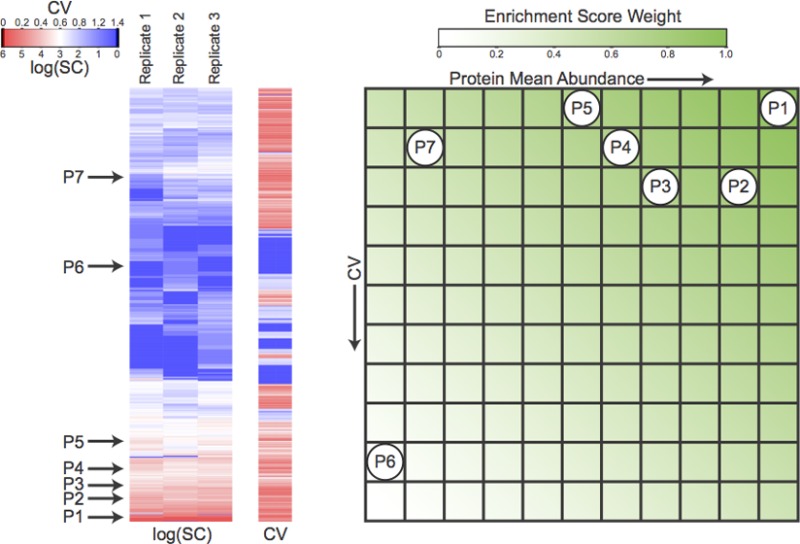
Figure 2.

Graphical representation of the PES calculation for label-free quantification. (A) Heat map representations of log normalized spectral counts log(SC) and normalized spectral count coefficients of variation (CV) for all proteins identified in the three biological replicates of the CFBE data set. A fictitious example of an annotation protein set of seven proteins is illustrated on the heat maps. (B) Color-coded representation of the enrichment score weight matrix W. Proteins p from the fictitious protein set in (A) are mapped onto W based on their respective protein mean abundances and abundance coefficients of variation CV_p^T. The sum of the enrichment score weights corresponding to their position in the matrix is then assigned as the PES of the fictitious protein set.

(2). Statistical Significance Assessment of PES

The statistical significance of the PES of a protein set S is computed using a Monte Carlo sampling procedure. Multiple alternative sampling procedures can be employed for this computation, each with their advantages and drawbacks.

(I). Uniform Sampling

The first Monte Carlo procedure called “uniform sampling” repeatedly samples a subset of |S| proteins in the analyzed data set, with each protein having an equal probability of being randomly sampled, and computes the PES for each of these random subsets to obtain an unbiased estimate of the PES distribution for |S| proteins. From this distribution, the p-value of a PES of a random subset can be computed representing the probability that it is larger or equal to the PES of S.

(II). Weighted Sampling

Although the uniform sampling method is unbiased, it ignores that proteins of high abundances are often those that have the most protein annotations and therefore belong to more protein sets. This is in part caused by the fact that these proteins are frequently those that are the most discussed in the literature, and also simply because some proteins perform more functions and are involved in more biological processes than others. This protein annotation bias could lead to an underestimation of protein set p-values, as heavily annotated proteins of high abundance will not be randomly selected as many times as they should. To correct this issue, we introduced a Monte Carlo “weighted sampling” procedure. This alternative method samples |S| proteins in the data set with a probability proportional to their respective number of occurrences in the ensemble of protein sets in the database (GO or MSigDB) being tested for enrichment. This approach models protein annotation biases and ensures more accurate p-value estimations, but could be slightly slower for large protein sets when the protein sampling probability distribution deviates greatly from the uniform distribution.

(III). Weighted and Uniform Sampling with Reduced Sample Space

These two sampling procedures implement a random selection of proteins in order to obtain the null distribution of PES. These methods assume among other things, that the abundances of proteins within the same protein set are independent. The validity of this assumption is debatable. This differs from the approach used by GSEA and PSEA, which avoids making such assumption and takes advantage of class label permutation (disease vs normal condition) in order to perform statistical assessments. As mentioned earlier, since proteomics data sets are often composed of experiments originating from a single condition, such permutation scheme is not always applicable. We therefore introduce a novel strategy, which consists of randomly selecting proteins using either the weighted or uniform sampling method in a reduced sample space. In an attempt to model protein abundance dependencies, we repeatedly sample |S| proteins at random and build the null distribution of PES using only samples for which the coefficient of variation of the mean abundances of sampled proteins falls within a user-defined range. This range is defined by applying a tolerance factor on the coefficient of variation of the mean abundances of the proteins in the protein set S, which is being statistically assessed. Specifically, Let C be the coefficient of variation of the ’s of the protein set S being statistically assessed and let 0 < f ≤ 1.0 be the coefficient of variance tolerance factor (CV tolerance). Let C′ be the coefficient of variation of the mean abundances of a randomly sampled protein set S′. Then, if f C ≤ C′ ≤ (1 + f)C, sample S′ will be used to build the null distribution of PES. Of note, this coefficient of variation C′ of the mean abundances of the proteins within a randomly sampled protein set is different from the coefficient of variation (CV_p) computed in the PES, which calculates the variation of the abundance measurements of a single protein across the replicate experiments. The reasoning behind this approach is that proteins in the same protein set are more likely to have similar abundances than randomly selected proteins (e.g., proteins that are members of the same protein complex), and therefore, protein abundances within such protein sets are more likely to yield a small coefficient of variation than a random set of proteins. While this approach does not model all protein dependencies within a protein set, it tackles an important issue and is likely to provide a more realistic estimate of the true distribution of PES. It should be noted that the sample space reduction by the CV tolerance can be applied to both the uniform and weighted sampling procedures presented above. Obviously, obtaining enough samples to produce a reliable null distribution of PES under this sampling method may require a longer running time depending on the CV tolerance that is selected by the user.

(3). False Discovery Rate Estimation

Since databases such as GO and MSigDB contain a large number of protein sets, multiple hypothesis testing correction of the above computed p-values is required. Because of the important dependencies and overlaps between the various protein sets, the computation of an empirical q-value (false discovery rate adjusted p-value) for each p-value is more appropriate than a too stringent Bonferroni correction. To estimate the empirical q-value for each protein set p-value, we randomize all protein sets and compute the protein set enrichment p-values of these random protein sets using steps (1) and (2) (see Methods). We propose three different randomization strategies in the Supporting Information. Let N(p) be the number of nonrandomized protein sets that obtained a p-value of at most p and R(p) be the number of randomized protein sets that are also associated with a p-value of at most p. We compute the false discovery rate (FDR) for all protein sets with a p-value ≤ p as FDR(p) = R(p)/N(p). FDR(p) may not be monotonic since it independently computes a FDR for each p-value threshold. We address this problem by setting FDR(p) = min_p′≥pFDR(p′). Such adjustment was proposed by Yekutieli and Benjamini to adjust p-values that were corrected for multiple hypothesis testing²⁸ and was applied in similar contexts.^29,30 Finally, for each protein set S with a p-value p_s, the empirical q-value is equal to FDR(p_s).

(4). Identification of Significant Protein Set Cores

A protein set S for which the proteins are significantly abundant and have a surprisingly small abundance coefficient of variation will obtain a small p-value and q-value. It does not, however, mean that all of the proteins in that protein set are abundant and have a small abundance coefficient of variation, but simply that a significant subset of S does. Let core(S) be such subset. We designed a greedy algorithm to identify core(S). The algorithm iteratively removes from S the protein for which the removal improves the p-value the most (i.e., protein with the minimum enrichment score weight) until no further p-value improvements can be performed. This greedy algorithm does not guarantee optimality but generally succeeds at identifying the key component of S.

Availability and Implementation

The proposed computational tools are implemented in a platform-independent Java program called PSEA-Quant. To decrease running time, PSEA-Quant first performs a presampling procedure where it estimates the p-value of a given protein set using a small number of random samples (100). If this p-value is less than 0.02, then the p-value estimation is refined using the user defined number of random samples. PSEA-Quant can be used on the web in a user-friendly fashion at krusty.scripps.edu:8080/PSEA-Quant or downloaded and used as a command-line tool at krusty.scripps.edu:8080/PSEA-Quant/files. The CFBE and human vs rat frontal cortex (HR) data sets are provided as sample input files at this address: krusty.scripps.edu:8080/PSEA-Quant/files. PSEA-Quant supports both UniProt³¹ identifiers and gene names as input.

Results

PSEA-Quant is an approach that identifies protein set annotations that are enriched for proteins with high abundance and low abundance measurement variation. In this paper, we applied PSEA-Quant using GO and MSigDB protein sets to a label-free quantified protein data set related to cystic fibrosis (CFBE) and to an isobaric labeling-based TMT quantified protein data sets of the frontal cortex of human and rat (HR) and human, mouse, and rat (HMR) brain. While TMT was used as an example of label-based quantification that can be used in conjunction with PSEA-Quant, it could have been replaced by any one of a number of other approaches such as iTRAQ, SILAC, or ¹⁵N. PSEA-Quant uses a variety of approaches to estimate the statistical significance of protein sets in a given data set and assigns them p-values. We validated these approaches by showing that the p-value distributions obtained with all techniques are largely uniformly distributed under the null hypothesis (see Supporting Information Figure S1 and text for complete analysis).

False Discovery Rate Analysis

Since a large number of protein sets are being tested for their enrichment (e.g., 8255 GO terms that were associated with at least two proteins in the CFBE data set), PSEA-Quant computes an empirical q-value for each protein set p-value. The results presented in Supporting Information Figure S1 highlighted that the protein number randomization technique is the most conservative randomization scheme and maintains protein annotation biases. It was therefore selected to estimate the false discovery rate and q-values in PSEA-Quant results. Figure 3 shows the FDR for small GO protein set p-values (≤ 0.01) obtained for the CFBE data set. There is a striking difference between the FDRs obtained for the same p-values between the uniform and weighted Monte Carlo sampling approaches. However, with both uniform and weighted sampling approaches, only the curves corresponding to a low CV tolerance (0.1) seem to behave slightly differently from the other ones obtained with the same sampling approach. Figure 3 demonstrates that for both sampling approaches, using a low CV tolerance is the most conservative approach, since it yields the highest FDR for the vast majority of p-values. The same observations can be made on the FDR curves of the Wild Type data set (Supporting Information Figure S2). Since we have described that the weighted Monte Carlo sampling technique models protein annotation biases and is therefore more likely to yield biologically significant results, and that a low CV tolerance (0.1) is the most conservative approach, these strategies are the ones that we used for the remaining data analyses in this article.

Figure 3.

FDRs associated with enrichment p-values computed by PSEA-Quant for the CFBE data set. The p-values were computed using the uniform and weighted Monte Carlo sampling procedures with mean abundance CV tolerance values of 1.0, 0.5, and 0.1 of the sampled protein sets (as described in Methods). When no CV tolerance was applied, the data are labeled as “Protein Independence”. FDRs were estimated using the “protein number randomization” strategy (as described in Methods).

PSEA-Quant Identifies Numerous GO Protein Sets Not Found to Be Significant Using GO Enrichment Analysis Tools

We compared the GO protein sets identified by PSEA-Quant in the CFBE data set (see Supporting Information File S1 for complete results) to those found to be enriched according to the GO enrichment analysis tools GOrilla¹⁰ and Ontologizer.⁷ There are several methods to analyze GO protein set enrichments. One could choose to test for the over-representation of a GO protein set in the entire data set based on what is expected in the Gene Ontology database. Another option is to set abundance and abundance coefficient of variation thresholds and test for the enrichment of GO protein sets within the subset of proteins passing these thresholds (proteins with the feature of interest), while using the entire data set as background. We ran GOrilla using the entire data set as a ranked protein list based on protein abundance and abundance coefficient of variation across replicates. We also executed GOrilla with thresholds on the protein abundance and abundance coefficient of variation across replicates so that the top 10% proteins were selected as having the feature of interest and the complete data set was considered as the background subset. The best p-value among the two GOrilla runs was considered for the benchmarking analysis (see Supporting Information Files S2 and S3 for complete results). In addition, we executed Ontologizer using the same top 10% protein subset and considering the complete data set as background. We also performed an Ontologizer analysis independently on each CFBE replicate using the entire GO database as background. We then associated the best p-value from all Ontologizer runs to each GO protein set (see Supporting Information File S4 and S5 for complete results). Table 1 shows the GO terms for which the protein sets were found to be significant according to PSEA-Quant (q-value < 0.1), but not by using the GOrilla and Ontologizer analyses (p-value ≥ 0.001). Interestingly, an important number of GO terms found by PSEA-Quant and not by GOrilla and Ontologizer are closely related to cystic fibrosis. Indeed, among the GO terms of interest, we find that proteins annotated with “glucose transport” (p-value = 2.0 × 10^–4 and q-value = 0.02) and “hexose transport” (p-value = 2.5 × 10^–4 and q-value = 0.03) are significantly abundant and that their abundance is measured with a surprisingly low coefficient of variation. These two biological processes have been shown to be disrupted in cystic fibrosis patients,^32,33 and glucose transport in particular is enhanced in various tissues of cystic fibrosis patients.^34,35 The leading cause of cystic fibrosis is the misfolding of CFTR caused by a deletion of F508 of the CFTR gene.^36,37 It is therefore not without interest that we observe that PSEA-Quant highlights GO terms, such as “protein binding involved in protein folding” (p-value = 6.0 × 10^–5 and q-value = 0.01) and “misfolded protein binding” (p-value = 9.9 × 10^–4 and q-value = 0.09), to be significant. It is also well described that sodium channels and chloride channels are disrupted in cystic fibrosis;^38,39 for instance, airway epithelia in cystic fibrosis patients have a higher rate of sodium absorption than normal.⁴⁰ Hence, to find “response to salt stress” (p-value = 2.3 × 10^–4 and q-value = 0.03) among the GO protein sets identified by PSEA-Quant is in accordance with the literature. Evidently, PSEA-Quant finds some GO protein sets that do not include a large number of proteins (see Table 1). However, these proteins are more abundant and their abundance measurements have a lower coefficient of variation than expected by chance. Both GOrilla and Ontologizer find several significantly enriched GO protein sets in our data that PSEA-Quant does not. This is expected since a GO protein set may be enriched in terms of number of occurrences in a data set, but not enriched for proteins of high abundance with well reproduced abundance measurements. The goal of PSEA-Quant is not to outperform tools like GOrilla or Ontologizer but rather to complement them. These differences in the results highlight the complementarity of the two strategies, where one analyzes the overrepresentation of a protein set in the data (GO analysis), and the other (PSEA-Quant) focuses on features of interest (e.g., abundance, abundance coefficient of variation, etc.) of the proteins associated with a protein set.

Table 1. Significant GO Terms Identified by PSEA-Quant (q-value < 0.1) and not Significant According to the GO Enrichment Analysis of Both Ontologizer and GOrilla (p-value ≥ 0.001) for the CFBE Data Set^a.

GO term	p-value	q-value	best Ontologizer p-value	best GOrilla p-value	GO term total size	number of proteins with GO term in CFBE data set
phosphopyruvate hydratase complex	<10–5	<0.01	0.237	>0.001	4	3
RNA splicing, via transesterification reactions with bulged adenosine as nucleophile	<10–5	<0.01	0.521	>0.001	218	148
UTP binding	3.0 × 10–5	0.01	0.009	>0.001	3	3
pyrimidine ribonucleoside binding	3.0 × 10–5	0.01	0.011	>0.001	3	3
nuclear envelope disassembly	4.0 × 10–5	0.01	0.057	>0.001	39	36
positive regulation of cell size	5.0 × 10–5	0.01	0.103	>0.001	8	3
protein binding involved in protein folding	6.0 × 10–5	0.01	0.020	>0.001	5	3
exopeptidase activity	7.0 × 10–5	0.01	0.016	>0.001	109	37
pyridoxal phosphate binding	8.0 × 10–5	0.01	0.015	>0.001	55	27
positive regulation of protein import into nucleus, translocation	9.0 × 10–5	0.01	0.011	>0.001	11	6
cell cortex part	1.7 × 10–4	0.02	0.005	>0.001	101	53
glucose transport	2.0 × 10–4	0.02	0.958	>0.001	118	35
fatty-acyl-CoA metabolic process	2.0 × 10–4	0.02	0.316	>0.001	26	11
response to salt stress	2.3 × 10–4	0.03	0.528	>0.001	22	6
hexose transport	2.5 × 10–4	0.03	0.342	>0.001	119	35
adenylate cyclase-activating G-protein coupled receptor signaling pathway	2.6 × 10–4	0.03	0.746	>0.001	52	6
NADP binding	2.9 × 10–4	0.03	0.053	>0.001	47	25
sarcoplasm	3.2 × 10–4	0.03	0.313	>0.001	61	3
transferase activity, transferring nitrogenous groups	3.2 × 10–4	0.03	0.052	>0.001	27	12
dATP binding	3.8 × 10–4	0.03	0.013	>0.001	4	4
cerebellar Purkinje cell layer development	4.7 × 10–4	0.03	0.030	>0.001	23	6
protein N-linked glycosylation via asparagine	4.7 × 10–4	0.03	0.052	>0.001	92	54
positive regulation of striated muscle contraction	5.0 × 10–4	0.03	0.034	>0.001	9	3
mRNA binding	6.1 × 10–4	0.05	0.031	>0.001	105	73
polypurine tract binding	6.2 × 10–4	0.06	0.044	>0.001	14	10
aminopeptidase activity	7.8 × 10–4	0.08	0.005	>0.001	36	19
GTPase inhibitor activity	8.0 × 10–4	0.08	0.017	>0.001	13	4
opsonin binding	9.2 × 10–4	0.09	0.348	>0.001	9	3
misfolded protein binding	9.9 × 10–4	0.09	0.283	>0.001	7	3

^aRedundant GO terms were removed and p-values and q-values were rounded.

PSEA-Quant Identifies Cystic Fibrosis Related GO Protein Sets That Are Differentially Expressed between the CFBE and Wild Type Data Set

As shown previously, PSEA-Quant found various significant GO protein sets that were relevant to cystic fibrosis when simply provided the CFBE data set as input. PSEA-Quant is capable of handling such a label-free quantified data set composed of a single condition, but it can also be extended to use a data set that includes a contrasting condition to produce biologically relevant results, even though it was not explicitly designed for this task. Table 2 shows the most significant GO protein sets using PSEA-Quant in the CFBE data set (q-value < 0.06) but not in the Wild Type data set (q-value ≥ 0.1). The vast majority of the GO protein sets discussed above was found to be significant in the CFBE data set (q-value < 0.1) and not in the Wild Type, with the exception of “glucose and hexose transport”, which was also significant in the Wild Type data set. In addition, this analysis highlighted other GO protein sets of interest. It should be noted that these supplementary GO protein sets were also found to be significant by GOrilla or Ontologizer. Among these we find the “COP9 signalosome” (p-value = 1.0 × 10^–5 and q-value < 0.01), which is very tightly involved in the degradation of CFTR.^41,42 “Cellular response to interleukin-4” (p-value = 1.0 × 10^–5 and q-value < 0.01) was also found as significant only in the CFBE data set. This result is consistent with the literature, which indicates that cystic fibrosis patients have an increased sensitivity to the cytokine interleukin-4.⁴³ On the other hand, Supporting Information Table S1 shows the most significant GO protein sets in the Wild Type data set (q-value < 0.03) (see Supporting Information File S6 for complete results) that are not in the CFBE data set (q-value ≥ 0.1). Among the GO terms of interest, we find “cell redox homeostasis” (p-value < 10^–5 and q-value < 0.01). Indeed, calcium homeostasis is known to be abnormal in cystic fibrosis airway epithelial cells.⁴⁴ The presence of the GO term “actin cytoskeleton” is also noteworthy since actin was reported to bind and potentially affect the functional properties of CFTR.⁴⁵ The results in Table 2 and Supporting Information Table S1 highlight that PSEA-Quant identifies protein sets that are of putative biological interest with regards to cystic fibrosis. Of note, it is not because the relationship between certain GO terms listed in Table 2 and Supporting Information Table S1 and cystic fibrosis is not obvious that these terms are irrelevant. These protein sets might prove themselves useful in order to understand the differences in the proteome between the CFBE and Wild Type samples. Further analyses could highlight the relevance of such GO terms. Figure 4 shows representative examples of GO terms and their protein sets that are related to cystic fibrosis for which the protein sets were classified as significant according to PSEA-Quant for the CFBE data set but not the Wild Type one.

Table 2. Top Significant GO Terms Identified by PSEA-Quant in the CFBE Data Set (q-value < 0.06) but Not Significant in the Wild Type Data Set (q-value ≥ 0.1)^a.

GO term	CFBE p-value	CFBE q-value	Wild Type p-value	Wild Type q-value	GO term total size	number of proteins with GO term in CFBE data set
catalytic step 2 spliceosome	<10–5	<0.01	0.002	0.16	80	73
regulation of apoptotic process	<10–5	<0.01	0.030	0.65	1162	418
cytosolic part	<10–5	<0.01	0.004	0.22	184	131
lyase activity	<10–5	<0.01	0.002	0.13	387	64
COP9 signalosome	1.0 × 10–5	<0.01	0.003	0.19	35	26
response to interleukin-4	1.0 × 10–5	<0.01	0.008	0.30	29	13
nuclear pore	2.0 × 10–5	0.01	0.009	0.33	67	49
nitric-oxide synthase regulator activity	4.0 × 10–5	0.01	0.001	0.11	6	4
negative regulation of cell cycle phase transition	5.0 × 10–5	0.01	0.103	0.91	172	97
negative regulation of dephosphorylation	6.0 × 10–5	0.01	0.250	1.00	6	5
exopeptidase activity	7.0 × 10–5	0.01	0.027	0.55	109	37
positive regulation of protein insertion into mitochondrial membrane involved in apoptotic signaling pathway	7.0 × 10–5	0.01	0.090	0.87	24	16
pyridoxal phosphate binding	8.0 × 10–5	0.01	0.050	0.76	55	27
antigen processing and presentation of peptide antigen	8.0 × 10–5	0.01	0.011	0.36	186	157
structural constituent of cytoskeleton	8.0 × 10–5	0.01	0.002	0.16	96	59
cell junction assembly	9.0 × 10–5	0.01	0.001	0.11	186	74
pyridine nucleotide metabolic process	1.2 × 10–4	0.01	0.017	0.44	52	28
pyrimidine nucleotide binding	1.4 × 10–4	0.02	0.020	0.48	8	5
fatty-acyl-CoA metabolic process	2.0 × 10–4	0.02	0.003	0.20	26	11
response to salt stress	2.3 × 10–4	0.03	0.030	0.65	22	6
signal sequence binding	2.3 × 10–4	0.03	0.022	0.50	21	12
positive regulation of protein modification process	2.5 × 10–4	0.03	0.030	0.65	803	273
adenyl deoxyribonucleotide binding	2.7 × 10–4	0.03	0.012	0.37	5	4
NADP binding	2.9 × 10–4	0.03	0.005	0.24	47	25
zona pellucida receptor complex	3.0 × 10–4	0.03	0.003	0.17	11	9
intracellular organelle part	3.1 × 10–4	0.03	0.007	0.28	6964	3132
response to endoplasmic reticulum stress	3.1 × 10–4	0.03	0.014	0.41	126	67
sarcoplasm	3.2 × 10–4	0.03	0.280	1.00	61	3
protein N-linked glycosylation	3.4 × 10–4	0.03	0.030	0.65	100	55
dATP binding	3.8 × 10–4	0.03	0.080	0.86	4	4
organic acid metabolic process	3.8 × 10–4	0.03	0.005	0.25	1042	382
ribosomal protein import into nucleus	4.2 × 10–4	0.03	0.009	0.33	4	4
positive regulation of cell cycle process	4.3 × 10–4	0.03	0.030	0.65	185	93
positive regulation of catalytic activity	4.3 × 10–4	0.03	0.015	0.43	1242	354
peptidyl-asparagine modification	4.4 × 10–4	0.03	0.050	0.76	93	55
cerebellar purkinje cell layer development	4.7 × 10–4	0.03	0.005	0.24	23	6
positive regulation of molecular function	4.7 × 10–4	0.03	0.030	0.65	1565	420
positive regulation of striated muscle contraction	5.0 × 10–4	0.03	0.002	0.15	9	3
oxoacid metabolic process	5.2 × 10–4	0.03	0.005	0.25	1026	378
calcium-dependent phospholipid binding	6.0 × 10–4	0.05	0.020	0.48	33	15

^aRedundant GO terms were removed and p-values and q-values were rounded.

Figure 4.

Scatter plot of the union of all proteins identified in all three replicates of the CFBE data set. The normalized spectral count coefficient of variation across all three replicates of each protein is plotted against its mean normalized spectral count. Proteins annotated with representative examples of GO terms related to cystic fibrosis identified as significant by PSEA-Quant in the CFBE data set, but not in the Wild Type one are color-coded. HSPA1A and HSP90AB1 are respectively colored in brown and purple due to their presence in more than one protein sets. Protein names in each protein set are listed. Protein names in bold correspond to proteins belonging to the core of a protein set.

PSEA-Quant Identifies Cystic Fibrosis Related MSigDB Protein Sets That Are Differentially Expressed between the CFBE and Wild Type Data Set

PSEA-Quant is not limited to the use of protein sets originating from the GO database. Indeed, any type of protein set from KEGG pathways⁶ to user-defined protein sets can be used as input for PSEA-Quant. To demonstrate this feature of our tool, we used PSEA-Quant to identify MSigDB protein sets that were significant in the CFBE (q-value < 0.1) but not in the Wild Type data set (q-value ≥ 0.1) (see Supporting Information File S7). Among the protein sets identified by PSEA-Quant, we find the curated protein set “CUI GLUCOSE DEPRIVATION” (p-value = 9.6 × 10^–4 and q-value = 0.07), which contains genes that are up-regulated under glucose-deprived conditions. This result is notable since, as discussed earlier, glucose transport is disrupted in cystic fibrosis cases. This analysis also allowed us to discover additional protein sets of interest that are related to cystic fibrosis. For instance, the curated protein set “PID HDAC CLASSII PATHWAY” (p-value = 1.5 × 10^–4 and q-value = 0.02) was found significant. This protein set includes genes involved in signaling events mediated by HDAC class II. Interestingly, HDAC7, a HDAC class II protein, is known to play a role in the restoration of the function of ΔF508CFTR.⁴⁵ In addition, PSEA-Quant identified the KEGG protein set: “GLUTATHIONE METABOLISM” (p-value = 3.1 × 10^–4 and q-value = 0.03). This observation is noteworthy since cystic fibrosis patients are known to be glutathione deficient.⁴⁶ Finally, the protein set “CAMP UP.V1 UP” (p-value = 3.0 × 10^–5 and q-value = 0.01), which contains genes that are up-regulated in response to cAMP signaling pathway activation, was also found to be significant in the CFBE data set. This result is interesting since CFTR is a cAMP-activated ATP-gated anion channel.⁴⁰

PSEA-Quant Highlights GO Protein Set Enrichment Differences between the Frontal Cortex of Human, Mouse, and Rat

PSEA-Quant was applied to both the human-rat (HR) and human-mouse-rat (HMR) TMT label-based quantification data set. Mice and rats are commonly employed to mimic neurological disorders due to the amazing conservation of the brain across mammalian species. Differences, however, do exist and understanding them can lead to improved animal models of diseases. GO protein sets identified as significantly up-regulated with a low coefficient of variation in human vs rat in the HR data set are shown in Table 3 (q-value < 0.01, see Supporting Information File S8 for complete results). Table 3 shows an important number of very significant GO terms related to mitochondria such as “NADH dehydrogenase activity”, “mitochondrion”, “mitochondrial ATP synthesis coupled proton transport”, “mitochondrial membrane”, and “mitochondrial electron transport, NADH to ubiquinone”. Obviously, while some are mostly independent, not all the protein sets associated with these GO terms are mutually exclusive. However, an important number of proteins related to mitochondria are significantly up-regulated in human vs the rat. Mitochondria are the main source of ATP in the brain but also possess other functions such as calcium homeostasis and regulation of apoptosis.^47,48 The ATP powers synaptic activity, ionic membrane gradients, propagation of action potentials, and axonal transport.^49,50 These results may potentially be explained by the fact that even if the rodent brain was the same size of the human, it would still possess only an eighth of the neurons in the human cerebral cortex.⁵¹ Therefore, this would also argue for a higher number of mitochondria in the human frontal cortex compared to rat to support the greater neuronal activity of the human brain. We observe a similar trend when analyzing with PSEA-Quant protein sets significantly up-regulated with a low coefficient of variation in human vs mouse in the HMR data set (Table 4). Of note, the results are extremely similar when performing the same analysis of human vs rat in the HMR data set (data not shown). These results are potentially interesting for many human specific neurological diseases, such as Alzheimer’s disease, Parkinson’s disease, schizophrenia, and depression, that are in part due to mitochondria dysfunction.⁵²⁻⁵⁴

Table 3. Top Significant GO Terms Identified by PSEA-Quant As Enriched for Upregulated Proteins with Low Coefficient of Variation in Human vs Rat in the Human and Rat (HR) Frontal Cortex TMT Protein Quantification Data Set (q-value < 0.01)^a.

GO term	p-value	q-value	number of proteins with GO term in HR data set
generation of precursor metabolites and energy	<10–5	<0.01	162
NADH dehydrogenase complex	<10–5	<0.01	33
single-organism biosynthetic process	<10–5	<0.01	146
cellular response to reactive oxygen species	<10–5	<0.01	35
response to hydrogen peroxide	<10–5	<0.01	39
oxidoreductase activity	<10–5	<0.01	291
mitochondrial part	<10–5	<0.01	409
monocarboxylic acid metabolic process	<10–5	<0.01	148
electron transport chain	<10–5	<0.01	63
organelle membrane	<10–5	<0.01	766
extracellular region	<10–5	<0.01	195
mitochondrial respiratory chain complex I	<10–5	<0.01	33
NADH dehydrogenase (ubiquinone) activity	<10–5	<0.01	28
respiratory chain complex I	<10–5	<0.01	33
response to wounding	<10–5	<0.01	98
response to ionizing radiation	<10–5	<0.01	21
cellular response to hydrogen peroxide	<10–5	<0.01	25
mitochondrion	<10–5	<0.01	649
antioxidant activity	<10–5	<0.01	34
lysosomal lumen	<10–5	<0.01	24
hydrogen ion transmembrane transporter activity	<10–5	<0.01	44
cellular modified amino acid metabolic process	<10–5	<0.01	81
mitochondrial ATP synthesis coupled proton transport	<10–5	<0.01	11
respiratory electron transport chain	<10–5	<0.01	63
vacuolar lumen	<10–5	<0.01	25
cytochrome c oxidase activity	<10–5	<0.01	14
peroxidase activity	<10–5	<0.01	18
mitochondrial membrane	<10–5	<0.01	262
oxidation–reduction process	<10–5	<0.01	245
mitochondrial electron transport, NADH to ubiquinone	<10–5	<0.01	26
bicarbonate transport	1.0 × 10–5	<0.01	6
cellular response to oxidative stress	1.0 × 10–5	<0.01	49
regulation of blood vessel size	1.0 × 10–5	<0.01	14
glutathione derivative metabolic process	1.0 × 10–5	<0.01	13
sterol metabolic process	1.0 × 10–5	<0.01	40
fatty acid catabolic process	1.0 × 10–5	<0.01	33
carboxylic ester hydrolase activity	2.0 × 10–5	<0.01	30
steroid metabolic process	2.0 × 10–5	<0.01	60
protein activation cascade	2.0 × 10–5	<0.01	13
lipid metabolic process	2.0 × 10–5	<0.01	321
organonitrogen compound biosynthetic process	3.1 × 10–5	<0.01	185
response to axon injury	3.1 × 10–5	<0.01	18

^aRedundant GO terms were removed and p-values and q-values were rounded.

Table 4. Top Significant GO Terms Identified by PSEA-Quant As Enriched for Upregulated Proteins with Low Coefficient of Variation in Human vs Mouse in the Human, Mouse, and Rat (HMR) Frontal Cortex TMT protein quantification dataset (q-value < 0.02)^a.

GO term	p-value	q-value	number of proteins with GO term in HMR data set
mitochondrial respiratory chain complex I	<10–5	0.01	38
NADH dehydrogenase (quinone) activity	<10–5	0.01	30
blood coagulation	<10–5	0.01	90
protein folding	<10–5	0.01	88
hydrogen ion transmembrane transporter activity	<10–5	0.01	48
mitochondrial electron transport, NADH to ubiquinone	<10–5	0.01	28
single-organism metabolic process	<10–5	0.01	1014
respiratory electron transport chain	<10–5	0.01	65
cofactor binding	<10–5	0.01	138
cytoplasmic membrane-bounded vesicle lumen	<10–5	0.01	25
catabolic process	<10–5	0.01	640
oxidoreductase activity, acting on NAD(P)H	<10–5	0.01	56
antioxidant activity	<10–5	0.01	33
mitochondrial membrane part	<10–5	0.01	105
extracellular matrix	<10–5	0.01	69
mitochondrion	<10–5	0.01	672
response to oxidative stress	<10–5	0.01	95
hemostasis	<10–5	0.01	92
cytosol	<10–5	0.01	765
monocarboxylic acid metabolic process	<10–5	0.01	147
organelle membrane	<10–5	0.01	738
intracellular organelle lumen	<10–5	0.01	178
platelet activation	<10–5	0.01	48
cell activation	<10–5	0.01	104
regulation of body fluid levels	<10–5	0.01	113
protease binding	<10–5	0.01	19
platelet degranulation	<10–5	0.01	28
mitochondrial part	<10–5	0.01	402
generation of precursor metabolites and energy	<10–5	0.01	151
carboxylic acid metabolic process	<10–5	0.01	336
oxoacid metabolic process	<10–5	0.01	351
melanosome	1.0 × 10–5	0.01	52
organic acid catabolic process	1.0 × 10–5	0.01	91
sulfur compound metabolic process	1.0 × 10–5	0.01	78
cellular amino acid metabolic process	1.0 × 10–5	0.01	186
lipid metabolic process	1.0 × 10–5	0.01	303
xenobiotic metabolic process	2.0 × 10–5	0.01	30
small molecule catabolic process	2.0 × 10–5	0.01	113
GTPase activity	2.0 × 10–5	0.01	113
organonitrogen compound metabolic process	2.0 × 10–5	0.01	558
cellular modified amino acid metabolic process	3.0 × 10–5	0.01	82
cell junction assembly	3.0 × 10–5	0.01	54

^aRedundant GO terms were removed and p-values and q-values were rounded.

In contrast, when looking for GO protein sets that are significantly upregulated with low coefficient of variation in the mouse and rat frontal cortices when compared to human, fewer GO protein sets were identified by the PSEA-Quant analysis of the HMR and HR TMT data sets (see Supporting Information Tables S2 and S3). Interestingly, although not extremely significant, both rodents when compared to human appear to have an overexpression of synapse and dendrite related proteins. It is worth noting that it is difficult to supply an explanation for certain GO terms identified by PSEA-Quant in this context since, to our knowledge, such protein quantification experiments across closely related species have never been performed. Variations in the expression of most biological mechanisms remain unknown across these species. Hence, some of the GO protein sets identified by PSEA-Quant in Supporting Information Tables S2 and S3 could be of putative biological interest. Also, as expected because of their evolutionary conservation, the analysis did not reveal striking differences in terms of GO protein set enrichments between the mouse and rat frontal cortices (see Supporting Information Tables S4 and S5), with the only major difference being that a number of laminins and collagens appear up-regulated in rat vs mouse. These cause some laminins and collagen related GO protein sets to obtain significant p-values according to PSEA-Quant.

Discussion and Conclusion

PSEA-Quant highlights protein sets of putative biological relevance that are not identified using classic GO enrichment analysis software packages. We believe that, when used in conjunction with such tools, PSEA-Quant facilitates the analysis of complex protein quantification data sets.

As mentioned previously, PSEA-Quant uses replicated experiments in order to identify protein sets of interest. A PSEA-Quant analysis requires a minimum of two replicates to compute an abundance coefficient of variation for each protein. Obviously, if more replicates are given as input to PSEA-Quant, it improves its capacity to differentiate proteins with different abundance variations. Our results show that three replicate label-free experiments were sufficient to obtain results of putative biological interest. As for isobaric labeled experiments, when two conditions were labeled with , two isobaric labels each (HMR data set), the resulting four abundance ratios, when used as input to PSEA-Quant, led to interesting results. Interestingly, the comparisons of the human and rat samples obtained similar PSEA-Quant results whether two (HMR) or three (HR) replicate samples for each species were labeled.

The nature of the replicates in a data set, biological or technical, is important to consider and affects the interpretation of the results of PSEA-Quant. When provided technical replicates as input, the PES computation of PSEA-Quant measures the mean abundance and the reliability of the abundance measurements of a protein with the coefficient of variation. Therefore, in this context PSEA-Quant identifies protein sets enriched for proteins of high abundance values measured with great reliability. When biological replicates are used as input to PSEA-Quant the PES reflects both the reliability of the abundance measurements and also the biological variability. Therefore, PSEA-Quant highlights protein sets containing proteins with surprisingly high and constant abundance whose abundance values are measured reproducibly across the biological replicates. In this scenario, one could expect matrix proteins such as actins to be among the top results. Even though this can be the case, our results clearly demonstrate that our method is sensitive enough to detect protein sets, which might be of greater biological interest. Nevertheless, the identification of protein sets containing proteins of high abundance with low abundance coefficient of variation is crucial to try to understand the biological processes taking place in a sample whether the sample is derived from an affinity purification, a whole cell extract, or a bodily fluid. In addition, the presence of matrix proteins among the top results can only arise when a single condition label-free quantified data set is given as input to PSEA-Quant. When samples that are quantified using a label-based approach or when a data set including two different conditions are given as input, matrix proteins tend to not appear in the results due to a lack of differential expression. Furthermore, this problem also occurs for the vast majority of GO analysis software packages currently available.

Although only spectral counts and TMT-labeled protein abundance ratios were used as input for PSEA-Quant in this paper, our approach can easily be applied to other protein quantification techniques such as iTRAQ, SILAC, and ¹⁵N. All of these methods perform a relative quantification of peptides and, therefore, proteins. Protein abundances obtained by these quantification approaches can be used to compute PES, the same way TMT protein abundance ratios were used in the present analysis. PSEA-Quant is also applicable to label-free and label-based protein quantification of proteins obtained through affinity purification coupled to mass spectrometry. Our software package can be particularly useful in such context to characterize the protein–protein interactions of a given protein.

Contaminants were not filtered from the data sets analyzed in this paper. We chose not to remove them to keep the analyzed data sets unbiased. In addition, we did not perform extensive noise processing of the analyzed data sets based on criteria such as number of peptides or spectra identified for a given protein. We opted not to do so to highlight the capabilities of PSEA-Quant, which can identify putative biologically significant protein sets in large noisy proteomics data sets. Nevertheless, PSEA-Quant might benefit from contaminant filtering and other sophisticated data set postprocessing techniques. Contaminant filtering may be particularly helpful before a PSEA-Quant analysis of proteomics experiments involving the use of antibodies such as affinity purification coupled to mass spectrometry. Indeed, protein nonspecific binding to antibodies could hinder the analytical power of PSEA-Quant. There are several publically available computational approaches that address this problem (SAINT,⁵⁵ CompPASS,⁵⁶ or Decontaminator⁵⁷) that could be used upstream of PSEA-Quant in the context of affinity purification coupled to mass spectrometry experiments. On the other hand, PSEA-Quant may in some cases be helpful to detect contaminants (see the Supporting Information).

Among the significant protein sets outputted by PSEA-Quant, some may share a number of proteins and therefore seem redundant. This problem would be important if the list of significant protein sets outputted by PSEA-Quant would be very long and tedious to analyze. This does not appear to be the case in the context of our present study. Nevertheless, in the future, we will propose methods to merge protein sets that share an important subset of proteins. Several methods that have been proposed to measure the distance or the semantic similarity between gene sets, such as the one from GO, will be explored.⁵⁸⁻⁶⁰

PSEA-Quant p-value estimation accuracy is limited by the number of samplings performed by the Monte Carlo procedure. To obtain an extremely high accuracy, a very large number of samplings is required, which in turn necessitates a considerable computational running time. Therefore, in the near future we will explore computational strategies, such as genetic algorithms, to accelerate PSEA-Quant and provide an even more accurate p-value estimator.

This paper focused on finding protein sets that were significantly enriched for proteins that are quantified with a low coefficient of variation and have a high abundance. However, one may not be interested in protein sets involving abundant proteins, but rather protein sets enriched for proteins with low abundance variance among a set of replicates. PSEA-Quant can easily be adapted to compute the significance of such protein sets by modifying the enrichment score weight matrix to only account for quantification reproducibility. Furthermore, the enrichment score weight matrix can be modified to consider additional features besides abundance and abundance coefficient of variation, such as the number of unique peptides detected or spectra intensities.

The ability to identify protein sets enriched for proteins with high abundance and reproduced quantification yields useful information about the proteome of a given sample. We firmly believe that methods such as PSEA-Quant will significantly improve our understanding of large quantification proteomics data sets. It will also provide helpful guidance to help formulate hypotheses about the biological mechanisms and processes taking place in a given sample.

Supporting Information Available

Table S1: Top significant GO terms identified by PSEA-Quant in the Wild Type data set but not in the CFBE data set. Table S2: Significant GO terms identified by PSEA-Quant in mouse vs human in the HMR data set. Table S3: Significant GO terms identified by PSEA-Quant in rat vs human in the HR data set. Table S4: Top GO terms identified by PSEA-Quant in mouse vs rat in the HMR data set. Table S5: Significant GO terms identified by PSEA-Quant in rat vs mouse in the HMR data set. Figure S1. Cumulative distributions of protein set enrichment p-values computed by PSEA-Quant for the CFBE data set using three randomized versions of GO assignments to proteins and different sampling strategies. Figure S2: FDRs associated to enrichment p-values computed by PSEA-Quant using different sampling strategies for the Wild Type data set. File S1: PSEA-Quant results for GO protein sets in the CFBE data set. Files S2 and S3: Enrichment p-values of GO terms provided by the GOrilla analyses of the CFBE data set. Files S4 and S5: Enrichment p-values of GO terms provided by the Ontologizer analyses of the CFBE data set. File S6: PSEA-Quant results for GO protein sets in the Wild Type data set. File S7: Significant MSigDB protein sets identified by PSEA-Quant in the CFBE data set but not in the Wild Type data set. File S8: PSEA-Quant results for GO protein sets for human vs rat in the HR data set. Files S9 and S10: UniProt identifiers exclusively contained in GO protein sets that are not significant in the CFBE data set (File S9) and in the Wild Type data set (File S10) according to PSEA-Quant. Files S11 and S12: List of proteins exclusively contained in MSigDB protein sets that are not significant in the CFBE data set (File S11) and in the Wild Type data set (File S12) according to PSEA-Quant. File S13: Intersection of the two lists of UniProt identifiers provided in Files S9 and S10. File S14: Intersection of the two lists of proteins provided in Files S11 and S12. Supporting Information Available: This material is available free of charge via the Internet at http://pubs.acs.org.

The authors declare no competing financial interest.

Funding Statement

National Institutes of Health, United States

References

- Subramanian A.; et al. Gene set enrichment analysis: a knowledge-based approach for interpreting genome-wide expression profiles. Proc. Natl. Acad. Sci. U.S.A. 2005, 102, 15545–15550. [DOI] [PMC free article] [PubMed] [Google Scholar]
- Anderle M.; Roy S.; Lin H.; Becker C.; Joho K. Quantifying reproducibility for differential proteomics: noise analysis for protein liquid chromatography-mass spectrometry of human serum. Bioinformatics 2004, 20, 3575–3582. [DOI] [PubMed] [Google Scholar]
- Griffin N. M.; et al. Label-free, normalized quantification of complex mass spectrometry data for proteomic analysis. Nat. Biotechnol. 2010, 28, 83–89. [DOI] [PMC free article] [PubMed] [Google Scholar]
- Ashburner M.; et al. Gene Ontology: Tool for the unification of biology. Nat. Genet. 2000, 25, 25–29. [DOI] [PMC free article] [PubMed] [Google Scholar]
- Liberzon A.; et al. Molecular signatures database (MSigDB) 3.0. Bioinformatics 2011, 27, 1739–1740. [DOI] [PMC free article] [PubMed] [Google Scholar]
- Kanehisa M.; Goto S. KEGG: Kyoto encyclopedia of genes and genomes. Nucleic Acids Res. 2000, 28, 27–30. [DOI] [PMC free article] [PubMed] [Google Scholar]
- Bauer S.; Grossmann S.; Vingron M.; Robinson P. N. Ontologizer 2.0 - A multifunctional tool for GO term enrichment analysis and data exploration. Bioinformatics 2008, 24, 1650–1651. [DOI] [PubMed] [Google Scholar]
- Al-Shahrour F.; Díaz-Uriarte R.; Dopazo J. FatiGO: A web tool for finding significant associations of Gene Ontology terms with groups of genes. Bioinformatics 2004, 20, 578–580. [DOI] [PubMed] [Google Scholar]
- Beißbarth T.; Speed T. P. GOstat: Find statistically overrepresented Gene Ontologies within a group of genes. Bioinformatics 2004, 20, 1464–1465. [DOI] [PubMed] [Google Scholar]
- Eden E.; Navon R.; Steinfeld I.; Lipson D.; Yakhini Z. GOrilla: A tool for discovery and visualization of enriched GO terms in ranked gene lists. BMC Bioinf. 2009, 10, 48. [DOI] [PMC free article] [PubMed] [Google Scholar]
- Zeeberg B. R.; et al. GoMiner: A resource for biological interpretation of genomic and proteomic data. Genome Biol. 2003, 4, R28. [DOI] [PMC free article] [PubMed] [Google Scholar]
- Mootha V. K.; et al. PGC-1α-responsive genes involved in oxidative phosphorylation are coordinately downregulated in human diabetes. Nat. Genet. 2003, 34, 267–273. [DOI] [PubMed] [Google Scholar]
- Subramanian A.; Kuehn H.; Gould J.; Tamayo P.; Mesirov J. P. GSEA-P: A desktop application for Gene Set Enrichment Analysis. Bioinformatics 2007, 23, 3251–3253. [DOI] [PubMed] [Google Scholar]
- Keller A.; et al. GeneTrailExpress: A web-based pipeline for the statistical evaluation of microarray experiments. BMC Bioinf. 2008, 9, 552. [DOI] [PMC free article] [PubMed] [Google Scholar]
- Keller A.; Backes C.; Lenhof H.-P. Computation of significance scores of unweighted Gene Set Enrichment Analyses. BMC Bioinf. 2007, 8, 290. [DOI] [PMC free article] [PubMed] [Google Scholar]
- Jiang Z.; Gentleman R. Extensions to gene set enrichment. Bioinformatics 2007, 23, 306–313. [DOI] [PubMed] [Google Scholar]
- Lee H. K.; Braynen W.; Keshav K.; Pavlidis P. ErmineJ: Tool for functional analysis of gene expression data sets. BMC Bioinf. 2005, 6, 269. [DOI] [PMC free article] [PubMed] [Google Scholar]
- Isserlin R.; et al. Pathway analysis of dilated cardiomyopathy using global proteomic profiling and enrichment maps. Proteomics 2010, 10, 1316–1327. [DOI] [PMC free article] [PubMed] [Google Scholar]
- Cha S.; et al. In situ proteomic analysis of human breast cancer epithelial cells using laser capture microdissection: Annotation by protein set enrichment analysis and gene ontology. Mol. Cell. Proteomics 2010, 9, 2529–2544. [DOI] [PMC free article] [PubMed] [Google Scholar]
- Fu X.; et al. Spectral index for assessment of differential protein expression in shotgun proteomics. J. Proteome Res. 2008, 7, 845–854. [DOI] [PubMed] [Google Scholar]
- Bell A. W.; et al. A HUPO test sample study reveals common problems in mass spectrometry-based proteomics. Nat. Methods 2009, 6, 423–430. [DOI] [PMC free article] [PubMed] [Google Scholar]
- Ong S.-E.; et al. Stable isotope labeling by amino acids in cell culture, SILAC, as a simple and accurate approach to expression proteomics. Mol. Cell. Proteomics 2002, 1, 376–386. [DOI] [PubMed] [Google Scholar]
- Ross P. L.; et al. Multiplexed protein quantitation in Saccharomyces cerevisiae using amine-reactive isobaric tagging reagents. Mol. Cell. Proteomics 2004, 3, 1154–1169. [DOI] [PubMed] [Google Scholar]
- Thompson A.; et al. Tandem mass tags: A novel quantification strategy for comparative analysis of complex protein mixtures by MS/MS. Anal. Chem. 2003, 75, 1895–1904. [DOI] [PubMed] [Google Scholar]
- Venable J. D.; Dong M.-Q.; Wohlschlegel J.; Dillin A.; Yates J. R. Automated approach for quantitative analysis of complex peptide mixtures from tandem mass spectra. Nat. Methods 2004, 1, 39–45. [DOI] [PubMed] [Google Scholar]
- Washburn M. P.; Ulaszek R.; Deciu C.; Schieltz D. M.; Yates J. R. Analysis of quantitative proteomic data generated via multidimensional protein identification technology. Anal. Chem. 2002, 74, 1650–1657. [DOI] [PubMed] [Google Scholar]
- Tian L.; et al. Discovering statistically significant pathways in expression profiling studies. Proc. Natl. Acad. Sci. U.S.A. 2005, 102, 13544–13549. [DOI] [PMC free article] [PubMed] [Google Scholar]
- Yekutieli D.; Benjamini Y. Resampling-based false discovery rate controlling multiple test procedures for correlated test statistics. J. Stat. Plann. Inference 1999, 82, 171–196. [Google Scholar]
- Käll L.; Canterbury J. D.; Weston J.; Noble W. S.; MacCoss M. J. Semi-supervised learning for peptide identification from shotgun proteomics datasets. Nat. Methods 2007, 4, 923–925. [DOI] [PubMed] [Google Scholar]
- Lavallée-Adam M.; et al. Discovery of Cell Compartment Specific Protein–Protein Interactions using Affinity Purification Combined with Tandem Mass Spectrometry. J. Proteome Res. 2012, 12, 272–281. [DOI] [PMC free article] [PubMed] [Google Scholar]
- Consortium U.; et al. The universal protein resource (UniProt). Nucleic Acids Res. 2008, 36, D190–D195. [DOI] [PMC free article] [PubMed] [Google Scholar]
- Baker E. H.; et al. Hyperglycemia and cystic fibrosis alter respiratory fluid glucose concentrations estimated by breath condensate analysis. J. Appl. Physiol. 2007, 102, 1969–1975. [DOI] [PubMed] [Google Scholar]
- Chace K. V.; et al. Respiratory mucous secretions in patients with cystic fibrosis: Relationship between levels of highly sulfated mucin component and severity of the disease. Clin. Chim. Acta 1983, 132, 143–155. [DOI] [PubMed] [Google Scholar]
- Baxter P.; Goldhill J.; Hardcastle J.; Hardcastle P. T.; Taylor C. J. Enhanced intestinal glucose and alanine transport in cystic fibrosis. Gut 1990, 31, 817–820. [DOI] [PMC free article] [PubMed] [Google Scholar]
- Beesley A. H.; Hardcastle J.; Hardcastle P. T.; Taylor C. J. Potassium and sodium dependent glucose transport: implications for cystic fibrosis. Arch. Dis. Child. 1997, 76, 477. [DOI] [PMC free article] [PubMed] [Google Scholar]
- Kerem B.; et al. Identification of the cystic fibrosis gene: Genetic analysis. Science 1989, 245, 1073–1080. [DOI] [PubMed] [Google Scholar]
- Cheung J. C.; Deber C. M. Misfolding of the cystic fibrosis transmembrane conductance regulator and disease. Biochemistry 2008, 47, 1465–1473. [DOI] [PubMed] [Google Scholar]
- Donaldson S. H.; Boucher R. C. Sodium channels and cystic fibrosis. CHEST J. 2007, 132, 1631–1636. [DOI] [PubMed] [Google Scholar]
- Zabner J.; Smith J. J.; Karp P. H.; Widdicombe J. H.; Welsh M. J. Loss of CFTR chloride channels alters salt absorption by cystic fibrosis airway epithelia in vitro. Mol. Cell 1998, 2, 397–403. [DOI] [PubMed] [Google Scholar]
- Stutts M. J.; et al. CFTR as a cAMP-dependent regulator of sodium channels. Science (80-.) 1995, 269, 847–850. [DOI] [PubMed] [Google Scholar]
- Gomes-Alves P.; Neves S.; Coelho A. V.; Penque D. Low temperature restoring effect on F508del-CFTR misprocessing: A proteomic approach. J. Proteomics 2009, 73, 218–230. [DOI] [PubMed] [Google Scholar]
- Wei N.; Serino G.; Deng X.-W. The COP9 signalosome: More than a protease. Trends Biochem. Sci. 2008, 33, 592–600. [DOI] [PubMed] [Google Scholar]
- Knutsen A. P.; et al. Increased sensitivity to IL-4 in cystic fibrosis patients with allergic bronchopulmonary aspergillosis. Allergy 2004, 59, 81–87. [DOI] [PubMed] [Google Scholar]
- Antigny F.; Norez C.; Becq F.; Vandebrouck C. Calcium homeostasis is abnormal in cystic fibrosis airway epithelial cells but is normalized after rescue of F508del-CFTR. Cell. Calcium 2008, 43, 175–183. [DOI] [PubMed] [Google Scholar]
- Chasan B.; et al. Evidence for direct interaction between actin and the cystic fibrosis transmembrane conductance regulator. Eur. Biophys. J. 2002, 30, 617–624. [DOI] [PubMed] [Google Scholar]
- Roum J. H.; Buhl R.; McElvaney N. G.; Borok Z.; Crystal R. G. Systemic deficiency of glutathione in cystic fibrosis. J. Appl. Physiol. 1993, 75, 2419–2424. [DOI] [PubMed] [Google Scholar]
- Chinopoulos C.; Adam-Vizi V. Calcium, mitochondria and oxidative stress in neuronal pathology. FEBS J. 2006, 273, 433–450. [DOI] [PubMed] [Google Scholar]
- Nagley P.; Higgins G. C.; Atkin J. D.; Beart P. M. Multifaceted deaths orchestrated by mitochondria in neurones. Biochim. Biophys. Acta, Mol. Basis Dis. 2010, 1802, 167–185. [DOI] [PubMed] [Google Scholar]
- MacAskill A. F.; Atkin T. A.; Kittler J. T. Mitochondrial trafficking and the provision of energy and calcium buffering at excitatory synapses. Eur. J. Neurosci. 2010, 32, 231–240. [DOI] [PubMed] [Google Scholar]
- Rawson R. L.; et al. Axons Degenerate in the Absence of Mitochondria in C. elegans. Curr. Biol. 2014, 24, 760–765. [DOI] [PMC free article] [PubMed] [Google Scholar]
- Herculano-Houzel S. The human brain in numbers: A linearly scaled-up primate brain. Front. Hum. Neurosci. 2009, 3, 31. [DOI] [PMC free article] [PubMed] [Google Scholar]
- Chaturvedi R. K.; Flint Beal M. Mitochondrial diseases of the brain. Free Radical Biol. Med. 2013, 63, 1–29. [DOI] [PubMed] [Google Scholar]
- Rezin G. T.; Amboni G.; Zugno A. I.; Quevedo J.; Streck E. L. Mitochondrial dysfunction and psychiatric disorders. Neurochem. Res. 2009, 34, 1021–1029. [DOI] [PubMed] [Google Scholar]
- Scaglia F. The role of mitochondrial dysfunction in psychiatric disease. Dev. Disability Res. Rev. 2010, 16, 136–143. [DOI] [PubMed] [Google Scholar]
- Choi H.; et al. SAINT: Probabilistic scoring of affinity purification-mass spectrometry data. Nat. Methods 2011, 8, 70–73. [DOI] [PMC free article] [PubMed] [Google Scholar]
- Sowa M. E.; Bennett E. J.; Gygi S. P.; Harper J. W. Defining the human deubiquitinating enzyme interaction landscape. Cell 2009, 138, 389–403. [DOI] [PMC free article] [PubMed] [Google Scholar]
- Lavallée-Adam M.; Cloutier P.; Coulombe B.; Blanchette M. Modeling contaminants in AP-MS/MS experiments. J. Proteome Res. 2010, 10, 886–895. [DOI] [PMC free article] [PubMed] [Google Scholar]
- Del Pozo A.; Pazos F.; Valencia A. Defining functional distances over Gene Ontology. BMC Bioinf. 2008, 9, 50. [DOI] [PMC free article] [PubMed] [Google Scholar]
- Jain S.; Bader G. D. An improved method for scoring protein-protein interactions using semantic similarity within the gene ontology. BMC Bioinf. 2010, 11, 562. [DOI] [PMC free article] [PubMed] [Google Scholar]
- Couto F. M.; Silva M. J.; Coutinho P. M. Measuring semantic similarity between Gene Ontology terms. Data Knowl. Eng. 2007, 61, 137–152. [Google Scholar]
Associated Data
This section collects any data citations, data availability statements, or supplementary materials included in this article.