

Abstract
The cross-validation deletion–substitution–addition (cvDSA) algorithm is based on data-adaptive estimation methodology to select and estimate marginal structural models (MSMs) for point treatment studies as well as models for conditional means where the outcome is continuous or binary. The algorithm builds and selects models based on user-defined criteria for model selection, and utilizes a loss function-based estimation procedure to distinguish between different model fits. In addition, the algorithm selects models based on cross-validation methodology to avoid “over-fitting” data. The cvDSA routine is an R software package available for download. An alternative R-package (DSA) based on the same principles as the cvDSA routine (i.e., cross-validation, loss function), but one that is faster and with additional refinements for selection and estimation of conditional means, is also available for download. Analyses of real and simulated data were conducted to demonstrate the use of these algorithms, and to compare MSMs where the causal effects were assumed (i.e., investigator-defined), with MSMs selected by the cvDSA. The package was used also to select models for the nuisance parameter (treatment) model to estimate the MSM parameters with inverse-probability of treatment weight (IPTW) estimation. Other estimation procedures (i.e., G-computation and double robust IPTW) are available also with the package.
Keywords: Cross-validation, Machine learning, Marginal structural models, Lung function, Cardiovascular mortality
1. Introduction
In recent years, epidemiologists’ knowledge about the theory and application of marginal structural models (MSMs) to examine causal effects in observational studies has grown substantially. MSMs provide unbiased estimates of marginal effects in the presence of both causal intermediates in point treatment (exposure) studies and time-dependent confounding in longitudinal studies (Robins et al., 2000). Conventional (conditional) association models provide stratum-specific effects which are typically biased in these situations. MSMs eliminate the need to adjust for confounding in the models themselves. Instead, nuisance parameter models (e.g. treatment models) are used to address confounding, so that with MSMs one obtains a direct, unconditional assessment of the exposure on the response. While model selection procedures for nuisance parameters have been addressed in the published literature (Mortimer et al., 2005; Brookhart and van der Laan, 2006), procedures for the selection of MSMs have not. The recent development of a general cross-validated data-adaptive model selection procedure represents an important methodological advancement to better characterize the causal effects of interest through MSM selection and a more flexible examination of the exposure–response causal curve.
The cross-validation deletion–substitution–addition (DSA) algorithm selects models adaptively for MSMs and nuisance parameter models for point treatment studies (Wang et al., 2004). The approach is derived from a general methodology that provides data-adaptive machine learning type algorithms based on user-supplied criteria (e.g., maximum model size) (van der Laan and Dudoit, 2003; Sinisi and van der Laan, 2004). Specifically, the algorithm builds a model space of candidate models based on so-called deletion, substitution and addition moves and utilizes a loss function-based estimation procedure to distinguish between different models with respect to model fit (van der Laan and Dudoit, 2003). The goal is to select a model that results in the best estimate of a given data distribution. Moreover, the algorithm selects models based partly on V-fold cross-validation (Efron and Tibshirani, 1993; Wang et al., 2004) and, thus, avoids the problem of “over-fitting” data that can occur with other data-adaptive model selection algorithms (e.g., StepAIC function, R-Software, current version, R Foundation for Statistical Computing).
This paper discusses methodological aspects of the algorithm and compares it with other model selection criteria. An illustrative analysis demonstrates how the algorithm works. Two R-packages are available which implement the algorithm: one is a well-developed package (DSA) for the selection of conditional models (e.g., nuisance parameter models); the second is for MSM selection for point treatment studies (cvDSA), and includes components for the selection of nuisance parameter models (cvGLM) and selection of MSMs (cvMSM). The second package (cvDSA) is less developed than the first in terms of ease of use and speed. We advise selection of the treatment model with the DSA package, and submission of this model to the cvMSM procedure for MSM selection. The discussion of the algorithm is in the context of its selection of MSMs, but it provides an overall view of the DSA algorithm as a general tool for model selection. Both packages are available for download from http://stat-www.berkeley.edu/~laan/Software/index.html. Additional background and technical details about the algorithm are available (Dudoit et al., 2003; van der Laan and Dudoit, 2003; Sinisi and van der Laan, 2004; Wang et al., 2004).
2. Background on MSMs
MSMs are used to define causal parameters of interest for exposure–response relations based on the concept of counterfactuals (Robins et al., 2000). This concept permits assessment of observational data in a hypothetical framework in which, contrary to fact, subjects were exposed to all possible levels of an exposure and had outcomes associated with those exposures. With counterfactual data, one can evaluate whether differences in the outcome are attributable to causal differences in the level of the exposure. To recreate the conditions under which observed data can be evaluated as counterfactual data requires several assumptions.
First, the observed data for any given subject represent one realization of his/her counterfactual data that correspond with the exposure actually received (consistency assumption) (Robins, 1999). In a point treatment study, the observed data can be represented as O = (W, A, Y = Y (A)), where W represents the baseline covariates, A the treatment (exposure) assignment, and Y (A) the outcome under observed treatment A. The observed data O = (W, A, Y ) on a randomly sampled subject represent one realization/component of the counterfactual “full” data X = ((Y (a), a ∈ A), W ) when exposure a = A.
A second assumption is the no “unmeasured confounders”, or “randomization assumption”: Y (a) ⊥ A|W – i.e., the treatment of interest is “randomized” with respect to the outcome within strata of the measured covariates, W (Robins, 1999). To satisfy this assumption, one conditions on all the measurable confounders of the exposure and outcome through a nuisance parameter model. Estimation of nuisance parameters can occur either by a model of a regression of the outcome on treatment (exposure) and all potential confounders (W ) (G-computation estimation, double robust inverse probability of treatment weight (DR-IPTW) estimation), or a model of the conditional probability of treatment given W (inverse probability of treatment weight (IPTW) estimation). Correct characterization of one of these nuisance parameter models is required to assess properly the effect of treatment on outcome without regard to potential extraneous factors.
Lastly, an additional assumption (experimental treatment assignment, or ETA) is required to provide unbiased estimates with IPTW estimation. This assumption states that all exposures have a positive probability of occurrence, given baseline covariates.
The parameter of interest in an MSM is the treatment-specific mean E(Y (a)|V ), possibly conditional on some baseline covariates V that are a subset of W (V ⊂ W ). When V = W, the MSM represents a traditional multiple regression model, where the effect of a is a fully adjusted causal parameter. Classical MSMs define a model for E(Y (a)|V ) such as a linear model m(a, V |β), so that the parameter of interest is the regression parameter β in this assumed model. The goal of the cross-validation DSA algorithm is to achieve a correct characterization (i.e., fit) of the nuisance models and MSMs to evaluate causal effects for point treatment studies.
Additional details of the theory and application of MSMs are available (Robins, 1999; Hernán et al., 2000; van der Laan and Robins, 2002; Yu and van der Laan, 2002; Haight et al., 2003; Neugebauer and van der Laan, 2003; Bryan et al., 2004; Mortimer et al., 2005).
3. Overview of the cross-validation deletion–substitution–addition algorithm
A possible estimator of the treatment-specific mean (MSM) minimizes the empirical risk – a statistical criterion of model fit defined below – over all candidate treatment-specific means. However, since the model space of possible treatment-specific means is infinite dimensional, given the different parameterizations of the treatment variable and the baseline covariates possible in the MSM, this minimization would simply result in an over-fit model. A general solution to deal with this problem is to construct a sequence or collection of subspaces (e.g., model categories of varying size and complexity) that approximate the whole model space, a so-called sieve; then, to compute the minimizers of the empirical risk for each of these subspaces. Application of V-fold cross-validation and a defined cross-validation risk criterion (described below) can be used to select the actual (optimal) subspace whose corresponding minimum empirical risk estimator minimizes the cross-validation risk (Fig. 1). Given that the process described above occurs in the framework of cross-validation, with the data subset into training/test data for purposes of selecting the optimal subspace, the process is repeated, and the construction of subspaces occurs based on a whole dataset. The minimizer of the empirical risk in the optimal subspace selected with cross-validation becomes the final selected model.
Fig. 1.

Overview of the cross-validation deletion–substitution–addition algorithm for model selection.
4. Key methodological aspects of the cross-validation DSA algorithm
Briefly, we describe some of the key aspects of the theory and methodology behind the cross-validation DSA algorithm in four areas: (1) loss functions as a measurement tool of model competency (e.g., model fit) for fitting the causal parameter of interest in the counterfactual world, and the basis by which these functions are applied to the observed data with the use of available mapping options for counterfactual data (e.g., G-computation, IPTW, DR-IPTW estimators); (2) two methods to estimate the loss function: empirical risk and cross-validation risk; (3) generation of candidate models; and (4) selection of nuisance parameter models. A detailed description of the mechanics of the DSA algorithm is provided in Appendix 1 and 2 (Appendix 1, 2 and 3 are included in the web version).
4.1. Loss functions and mapping of counterfactual data
Loss functions are criteria used in statistics to evaluate and to compare models based on fits of candidate estimators to data (Bickel and Doksum, 2001). With these criteria, and under the assumption that the class of models is an appropriate summary of the data, the goal of selection of a well-fit model occurs by minimization of the expectation of the loss function, or empirical risk, that can be represented generically as
with observations Oi on which a candidate model ψn is fit. A simple example of a loss function is the squared residual of an observed outcome and the predicted value that has the property that its expectation is minimized by the true conditional mean of the outcome, given the covariates. This loss function is thus suitable for regression. In fact, our nuisance parameter model selection for fitting the conditional mean of the outcome, given exposure and baseline covariates, and for fitting a regression of the exposure on the baseline covariates, is based on this loss function. Another example of a loss function is the minus log likelihood function that has the property that its expectation is minimized by the true density of the data. This is a loss function for model selection for the conditional distribution of a binary outcome, given baseline covariates. These two loss functions are simple in that they are known functions of the data structure and a candidate model for the parameter of interest.
The cross-validation DSA algorithm is based on the estimation of the expectation of loss functions (i.e., risk) where the loss function is a function of the observed data structure O = (W, A, Y ) and a candidate MSM for the causal parameter of interest. These loss functions are selected such that their expectation measures the discrepancy between a candidate fit of the causal parameter of interest for different models to the observed data and the true causal parameter (i.e., a perfect fit of a true model to the data).
The true causal parameter is the “absolute” minimizer of the expectation of the loss function (i.e., the risk function). However, in the real world, the true causal parameter is unknown. The goal of selection of the best estimator (i.e., the best candidate model) is to find the estimator closest to the true causal parameter. Since the unknown, true causal parameter gives a fixed risk (which is also unknown), the goal is simply to minimize the risk over all candidate model-specific fits of the causal parameter of interest. This can be achieved approximately by minimization of the empirical risk (i.e., the empirical mean of the loss function).
Another characteristic of loss functions particular to MSMs is the uniqueness of the data structure (i.e., counterfactual as compared with observational data) with which they are computed. If we could observe the counterfactual data X on each subject, we could choose as the loss function for the treatment-specific mean (MSM), possibly conditional on some baseline covariates V, the summed (over all possible exposures, (a), squared residuals between the counterfactual outcomes under treatment a and a candidate fit of the treatment-specific mean: L(X, ψ) = Σa∈A(Y (a) − ψ (a, V ))2. This loss function is the standard loss function for repeated measures regression in which each subject has multiple possible outcomes. Indeed, the expectation of this loss function is minimized at the true treatment-specific mean of the outcome (i.e., the causal parameter of interest). However, this loss function is not appropriate for the data we typically observe (i.e., a single counterfactual outcome that corresponds to a one-time exposure for a given individual).
van der Laan and Robins have presented a method to map counterfactual data-estimating functions to observed data-estimating functions with the same expectation; this method has direct implications for mapping counterfactual data loss functions to loss functions for observed data that can be carried out with any one of the three MSM estimators: G-Computation, IPTW, and DR-IPTW (van der Laan and Robins, 2002; Wang et al., 2004). For example, mapping of the loss functions based on the IPTW estimator is formulated as
where g(A|W ) and g(A|V ) are models for the treatment (exposure). The expected values of this IPTW loss function and the loss function for the counterfactual data are equivalent when we assume no unmeasured confounders. The DR-IPTW loss function not only provides a correct model specification for the treatment-specific mean (as the IPTW loss function), but it does so with minimum variance (van der Laan and Robins, 2002). Thus, the loss functions that are used typically in conventional analyses to evaluate models can be extended to evaluate and compare MSMs by mapping them into observed data loss functions with the G-computation, IPTW or DR-IPTW estimators. The details of the G-computation and DR-IPTW loss functions are provided in Appendix 1.
As stated above, given that the model space of potential candidate models is infinite dimensional, selection of these models based on minimization of the empirical risk alone would result in over-fit models. Fine-tuning parameters that describe the size and complexity of the model need to be based on the so-called cross-validation risk. Details of the formulation and application of cross-validation risk as a model selection criterion, in connection with empirical risk, in the cross-validation DSA algorithm are given below.
4.2. Comparison of empirical risk and cross-validation risk used in the cross-validation DSA algorithm
The algorithm uses a combination of both empirical risk and cross-validation risk criteria that operate jointly to evaluate and select models for the nuisance parameters (appropriate estimators of the MSM–i.e., controls for confounding) and the MSMs themselves. The process by which models are built, compared, and selected, based on minimization of the empirical risk, is done in the framework of V-fold cross-validation. After models are selected (based on empirical risk) that are representative of the different subspaces (approximate the whole model space) based on training data subsets of the entire data, they are fit with the remainder of the data (corresponding validation data of those training data subsets). The model corresponding to one of the subspaces (e.g., a model with five terms and no interactions) that minimizes the empirical mean over the different validation datasets – i.e., cross-validation risk average – is used to select the optimal subspace. The following description elaborates more on this process.
4.2.1. Cross-validation risk
Candidate models of the causal parameter of interest are selected by the DSA algorithm based on lowest empirical risk estimated from training data for different model size-complexity combinations. These different size-complexity combinations are referred to as subspaces. Since a model of optimal size and complexity cannot be selected based on the empirical risk (i.e., a model of maximum size-complexity would be selected), the cross-validation risk is used to select the size and complexity, within bounds set by the user. Cross-validation risk estimates are obtained for these selected models, indexed by size and complexity, based on validation data. For example, a candidate model is estimated with the observations in the training set; then, the empirical mean is taken over the validation set of the loss function at the candidate fit. This consecutive process can be described as a “one-step cross-validation risk”, which we define as the empirical mean (average) of the loss function over a validation sample. In the 5-fold cross-validation process, five one-step cross-validation risks are calculated for the different training–validation dataset combinations. A final cross-validation risk is calculated from an average of the five one-step cross-validation risks. It is well known that V-fold cross-validation provides a better estimate of true risk than a single split of the data.
In summary, the cross-validation DSA algorithm maps a training dataset into a set of models that are the optimal models of the subspaces in which these models occur. These models, in turn, are applied to a validation dataset to assess the cross-validation risk for each subspace that each model represents. The process is repeated for V-fold divisions of the whole dataset. At the end, the subspace with the lowest average cross-validation risk is selected as the optimal subspace. The final implementation of the cross-validation DSA algorithm on the whole dataset provides a set of best models that correspond to each subspace. The final optimal model is the one among these best models that occurs in the optimal subspace (see Fig. 1).
5. Generation of candidate estimators with the DSA algorithm
In the DSA algorithm, the whole model space is parameterized as a transformation (e.g., identity or logit function) of linear combinations of basis functions. The choices of the basis functions include the polynomial powers (i.e., 1, x, x2, …), and spline functions of fixed degree with corresponding fixed set of knot points and wavelets functions. This choice of a class of basis functions can itself be chosen with cross-validation. The current approach of the DSA algorithm is focused on use of the polynomial powers as the basis function.
Given this parameterization, the subspaces are obtained by restrictions on different conditions, i.e., the number of terms that a model contains (k1), maximum order of interactions (k2), etc. An example of such a subspace might be models that are polynomial functions of five terms and up to 3-way interactions. The best subspace, indexed by {k1, k2}, is selected with V-fold cross-validation. The final model fit is the one that minimizes the empirical risk, based on all the sample data over the subspace selected with V-fold cross-validation.
The minimization in the sequence of subspaces is accomplished with the DSA algorithm. The intuitive idea is that the algorithm searches for a better model in the ‘neighborhood’ of a ‘current best model’–e.g., A + AV1 + V2. This ‘neighborhood’ is defined as the deletion, substitution and addition sets of the current best model. Given the current best model above with k = 3 terms, the deletion set contains models of size k − 1 terms, by deletion of one of the k terms from the current model and keeping the other terms (e.g., AV 1 + V2). The substitution set contains models of the same size k (e.g., A2 + AV1 + V2), where each of the k terms is replaced by a new term, respectively. The addition set contains models of size k + 1, by adding a new term (a single variable or a new term generated by substitution) to the current model (e.g., A + AV1 + V2 + V1).
To evaluate models, the algorithm starts with an intercept model of size k = 0. Then the algorithm performs an addition move, where only a main effect term is added each time (the addition set of the current intercept model only includes main effect terms). The best model of size k = 1 is the one that has the minimal empirical risk (mean squared residual) among all the univariate models. The minimal empirical risk and the best model of size k = 1 are then saved.
Next, since there is only one term in the model, the algorithm carries out a substitution move. At this point, the algorithm is not interested in the deletion set that returns to the intercept model, and may conduct additional substitutions with interaction terms depending on the number of n-way interactions specified by the user. Within the substitution set, the substitution move finds the minimal empirical risk and its corresponding model and compares this minimal empirical risk with the previously saved minimal empirical risk of size k = 1. If the empirical risk of the substitution move is less, the minimal empirical risk and the best model of size k = 1 will be updated and a new round of substitution begins. If the empirical risk of the substitution move is not less than the saved empirical risk, the algorithm will keep the previous model and go to an addition move by adding a second term.
Once there is more than one term (exclusive of the intercept) in the model, the algorithm will perform a deletion move first. The deletion move finds the minimal empirical risk and its corresponding model within the deletion set and compares this minimal empirical risk with the previously saved minimal empirical risk of size k = 1. If the empirical risk of the deletion move is less, the minimal empirical risk and the best model of size k − 1 will be updated and the algorithm goes back to a new round of deletion moves (i.e., if there are at least two terms left in the model) or substitution moves (if only one term is left in the model). If the empirical risk of the deletion move is not less than the saved empirical risk of k − 1, the algorithm will keep the previous model and go to a substitution move. Addition moves will be considered up to a maximum model size as specified by the user. The DSA algorithm reports the best model for each size k.
If the subspace also is restricted by maximal order of interactions (e.g., 2-way interaction or 3-way interaction), the deletion, substitution and addition sets are generated under this additional restriction. For example, if the allowed maximal interaction is 3-way interaction, then the DSA algorithm will be carried out three times; first, for models with no interactions; second, for models that include 2-way interactions; finally, for models that include 2-way and 3-way interactions. The DSA algorithm returns the best models for all possible combinations of size and level of interaction allowed by the user.
6. Data-adaptive estimation of nuisance parameter models
Since the estimation of MSMs depends on nuisance parameter models, it should be emphasized that the cross-validation DSA algorithm needs to be applied to select these models as well, if they are unknown. Selection of a model (i.e., estimator) can occur by a number of different approaches. In each case, the selection of the model precedes the fit of the MSM. One approach to selection of the model (e.g., IPTW estimator) is through an integrated step within the cvMSM component of the cvDSA procedure, described in Section 1. Specifically, the training sample that is used to fit a candidate MSM is treated as a whole sample and is split into a number of subsets. Each of these subsets represents training and validation datasets at the level of the fit and selection of the treatment model. Once a candidate treatment model is selected through this process, it is used to estimate the candidate MSM. Other approaches to the selection of the IPTW treatment model, as well as other estimators, are the cvGLM procedure, available with the cvDSA package, or the alternative R-package (DSA) which is used to fit conditional models exclusively. These models would be submitted directly to the cvMSM.
In practice, when one considers treatment models, one examines the association of the outcome variable with each covariate that one considers a potential confounder of the causal effect. Only those variables that are associated with the outcome (e.g., p < 0.2) are included in the selection of the treatment model.
Different criteria can be used to select treatment models. For example, a model selection criterion was proposed to select the treatment model by minimizing the mean-squared error of the estimator of the MSM (Brookhart and van der Laan, 2006). However, this joint selection of the treatment and MSMs is not implemented in the current cvDSA R-package. Instead, the criterion used to select treatment models is based on a simpler set of computations which involve minimization of the cross-validated mean-squared error of the treatment model itself.
Ultimately, selection of one of the available estimators depends on which among them can provide consistent MSM estimates. Also, the fit of the MSM will depend on the fit of the nuisance model given the extent of the data to address the ‘no unmeasured confounders’ assumption and the selection criteria provided by the user to the algorithm.
7. Assessment of the cross-validation DSA algorithm for model selection
7.1. Overview
Simulations were carried out to assess the performance of the cross-validation DSA algorithm for the selection of both conditional models and MSMs under a variety of controlled conditions. Data were typically generated based on a random model (e.g., Y ~ X), where the set of covariates X (e.g., x1−x4) was comprised of random uniform variables, and the parameter values in front of the Xs were generated randomly from the uniform distribution. Random error was incorporated as part of the model as well. The DSA algorithm was utilized to select models closest to the models that generated the data – i.e., to select the model Y ~ X, for several replicates of data. The bias and mean square error (MSE) were determined for the different DSA-selected models to assess the model proficiency for each of these replicates.
A similar approach was taken to assess the DSA selection of MSMs; however, in addition, a binary treatment variable was generated, and the data were simulated to invoke confounding between this treatment variable and the outcome Y. In addition, this latter simulation included comparisons of the bias and MSE between MSMs selected by DSA and arbitrary, assumed MSMs, for the different simulated data.
Modifications were made to this overall scheme to assess the cross-validation DSA algorithm. Details that pertain to each of the different simulations are given below. Results of the simulations are provided in Tables 1a and 1b, and Figs. 2–5. The results are explained in Section 7.3.
Table 1a.
Representative DSA selections of conditional models and measures of model proficiency based on simulation studies 1–3.
| Study | N | σ | Data-generating model | DSA-selected model | Bias | MSE | |
|---|---|---|---|---|---|---|---|
| 1 | 500 | 0.25 | −1 + x1 + x2 + x1x3 | −1.04 + 1.05x1 + 1.04x2 + 0.91x1x3 | 0.014 | 0.055 | |
| 1 | 1000 | 1.00 | −1 + x1 + x2 + x1x3 |
|
−0.044 | 0.999 | |
| 2 | 500 | 0.25 | −9.09 + 0.96x2a | −9.09 + 0.95x2 + 0.06x3b | −0.015 | 0.060 | |
| 2 | 1000 | 1.00 | −5.65 + 7.04x1x3 | −5.64 + 7.09x1x3 − 0.02x1x2b | 0.034 | 1.008 | |
| Selection specificityc | |||||||
| 3 | 500 | 1.00 | 8.72 − 8.98x4 − 1.22x9d | 7.63 − 9.00x4 − 1.33x9 | −0.038 | 0.945 | |
| 3 | 1000 | 1.00 | 5.03 + 2.86x5 | 6.55 + 2.90x5 | −0.019 | 0.978 | |
| Selection sensitivityc | |||||||
| 3 | 500 | 1.00 | 6.63−4.55x4 − 2.54x7 + 4.77x9 − 4.63x10d | 7.52−4.67x4 − 2.40x7 + 4.67x9 − 4.62x10 | 0.056 | 1.049 | |
| 3 | 1000 | 1.00 | 4.36 − 0.56x1 − 2.40x8 − 4.32x9 + 9.09x10 | 4.58−0.59x1 − 2.34x8 − 4.30x9 + 9.08x10 | −0.026 | 0.999 | |
Signs for x1 and x1x3 were randomly set to 0; signs could be randomly set to −1, 0, or 1 times the parameter value that was randomly assigned for each term.
Additional but negligible terms represent some of the non-specific noise which the algorithm specified as part of the model.
Specificity and sensitivity represent the algorithm’s capacity to select smaller and larger (e.g., 4-term and 10-term) models given an expanded list of covariates and increased maximum model size to search and select models.
Coefficients for the different terms that do not appear in data-generating model were randomly set to 0. Other data-generating models used in the simulation would have included coefficients and terms that do not appear here.
Table 1b.
Representative comparison of DSA-selected and fixed (assumed) MSMs and measures of model proficiency based on Simulation Study 4 with varying conditions.
| Conditiona | Model | Bias | MSE | |
|---|---|---|---|---|
| Baseline levels of confounding and random noiseb | ||||
| True MSMc | 7.56 + 9.68A + 9.10x2 + 2.87Ax1 | |||
| DSA-selected | 7.56 + 9.67A + 9.12x2 + 2.85Ax1 | −0.006 | 0.064 | |
| Fixed MSM | 6.85 + 11.11A + 1.41x1 + 9.12x2 | −0.004 | 0.242 | |
| Increased confounding and baseline random noised | ||||
| True MSM |
|
|||
| DSA-selected |
|
−0.003 | 0.055 | |
| Fixed MSM | 0.94 + 2.05A + 3.05x1 + 4.62x2 | 0.014 | 0.118 | |
| Baseline confounding and increased random noisee | ||||
| True MSM |
|
|||
| DSA-selected | 2.00 + 2.02A + 4.26x2 + 0.46Ax1 | 0.019 | 1.012 | |
| Fixed MSM | 1.85 + 2.22A + 0.35x1 + 4.27x2 | 0.004 | 1.010 | |
Results are based on N = 500 with varying conditions (levels) of confounding and random error.
Baseline levels of confounding represented by g(A|X) = 0.9 + x1 + 0.5x2 − 1.3x1x3 and random error σ = 0.25 were incorporated in simulated data.
MSM used to generate the simulated data.
Increased levels of confounding represented by g(A|X) = 0.9 + 3x1 + 1.5x2 − 1.3x1x3 were incorporated in simulated data.
Increased levels of random error defined by σ = 1.
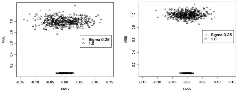
Fig. 2.

Bias and MSE of DSA-selected models based on 500 replicates of simulated data given varying conditions (sample size: N = 500 (top left); 1000 (top right); 5000 (bottom) and underlying variance σ ) where the data-generating model was a fixed model (Simulation Study 1).
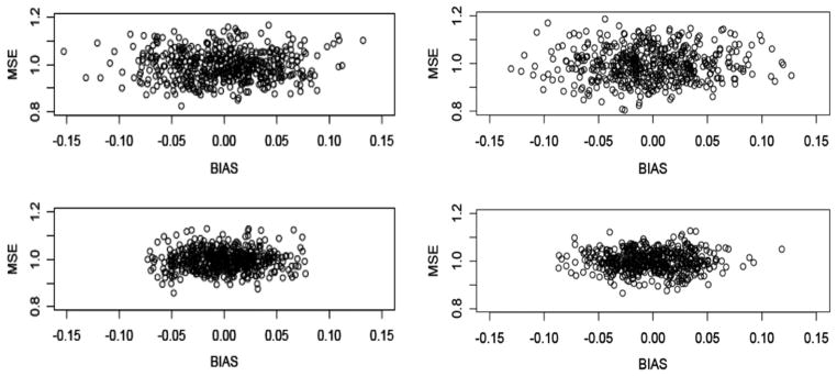
Fig. 5.

Bias and MSE of DSA-selected MSMs (left) and fixed (user-specified) MSMs (right) based on 200 replicates of data for varying conditions: baseline levels of confounding and random error (first row); increased confounding (second row); and increased random error (third row)).
7.2. Simulation methods
7.2.1. Simulation study 1
This simulation evaluated DSA model selection in the presence of varying sample size and random noise (error). The simulated data were based on four covariates x1−x4, all random uniform, and a fixed data-generating model for Y : − 1 + x1 + x2 + x1x3 (see Table 1a, Study 1). Datasets of different sizes N (i.e., 500, 1000, 5000) were generated, and random error was added to the outcome Y based on the standard normal distribution with standard deviation σ (i.e., 0.25, 0.5, and 1.0), in separate instances.
The DSA algorithm for selection of conditional models was used, and the selection criteria that were submitted included 5-fold cross-validation; a maximum model size = 4; orders of interaction = 2; and maximum sum of polynomial order or interaction = 2. An illustration of how these selection criteria are submitted to the algorithm is provided in Appendix 3.
The bias of each selected model was estimated based on the difference E(θ) – E(θ′), where θ represents the vector of predicted values based on the data-generating (‘true’) model and θ′ represents the vector of predicted values based on the DSA-selected model. The MSE was calculated as Bias2 + variance, where the variance was estimated as Σ(Y – θ′)2/(n – p), where Y represents the vector of observed responses, n is equal to the number of observations, and p is equal to the number of parameters in the DSA-selected model.
7.2.2. Simulation study 2
This particular simulation assessed DSA model selection where random models were used to generate the simulated data. Again, DSA model selection was evaluated given different sample sizes and random error imposed on Y. The simulated data were based on four covariates x1−x4, as in the previous simulation, except the data-generating model for Y was not fixed but random for each simulated dataset (see Table 1a, Study 2). Values of the coefficients in the random models were generated from the uniform distribution, and the signs in front of the coefficients (−1, 0, 1) were randomized. Datasets based on different sample sizes (i.e., 500, 1000) were generated, and random error σ (i.e., 0.25, 1) was assigned. The selection criteria submitted to the algorithm were the same as those used in the previous simulation. The bias and MSE were determined for each of the models selected as described above.
7.2.3. Simulation study 3
This next simulation assessed the specificity and sensitivity of DSA model selection. The simulated data were based on additional covariates x1−x10, where some of these covariates were random binary variables. The data-generating model for Y was not fixed but random for each simulated dataset (see Table 1a, Study 3). In addition, the data-generating model consisted of 4 terms or 10 terms, in separate instances, to determine how well the DSA algorithm selected a smaller model (specificity) or a larger model (sensitivity) given the additional covariates that were added as part of the simulation. The simulation was evaluated in the context of varying sample sizes (i.e., 500, 1000), with the same random error (i.e., σ = 1) assigned to Y. One model selection criterion was modified from the previous simulations by an increase in the maximum model size from 4 to 10. The bias and MSE were calculated as previously described for each of the selected models.
7.2.4. Simulation study 4
This last simulation examined the performance of the cross-validation DSA algorithm to select MSMs. The simulated data were based on a few covariates (x1−x4), and a binary treatment variable whose values (A = 0, 1) were assigned based on a linear combination of covariates (i.e., 0.9 + x1 + 0.5x2 − 1.3x1x3), to invoke confounding between A and Y. Random error was incorporated also as part of the treatment assignment. The data-generating model for Y (an MSM) was not fixed but random for each simulated dataset that was generated (see Table 1b). Each model consisted of the binary treatment variable, and two covariates (x1, x2) to represent V in the MSM. Parameter values of the different model terms were based on values generated at random from the uniform distribution. The simulation was designed so that x1 appeared randomly in the model as either a square term or as part of an interaction with A (i.e., , Ax1, respectively). The cross-validation DSA algorithm was used to choose models closest to those used to generate data. By way of comparison with the DSA-selected MSMs, we fit fixed, misspecified (i.e., assumed) MSMs to the data which included the treatment variable, and x1 and x2 as singular, first-order terms only.
All datasets in this simulation were of equal sample size (N = 500), and constant random error (σ = 0.25) was added to the outcome Y. Different situations characteristic of MSM analyses were incorporated to assess the adaption of the DSA algorithm to these different circumstances. For example, confounding (i.e., 0.9 + 3x1 + 1.5x2 − 1.3x1x3), and random error (σ = 1) were increased in separate simulations. Given the additional time required to select MSMs with the DSA algorithm, 200 rather than 500 replicates of data employed in the previous simulations were used to examine the distribution of bias and MSE for the different selected models.
The model selection criteria used as part of cvMSM() included 5-fold cross-validation; a maximum model size = 4; orders of interaction = 2; and maximum polynomial order of the different terms = 2. The model for A given the covariates (e.g., A ~ X) provided above was submitted to the algorithm, as well as a model A ~ V, where V = x1, x2. The models were fit with IPTW estimation which included the option for stabilized weights.
7.3. Simulation results
Tables 1a and 1b contain representative models from the different simulations and illustrate the extent to which models selected by the DSA algorithm approximate those that were used to generate the actual data. Measures of bias and mean square error (MSE) summarize the differences based on the models selected by the DSA algorithm and the true models of the data. Particular conditions are shown (Tables 1a and 1b, far left column) to illustrate how model selection depends on the sample size and random variability of the data. Tables 1a and 1b provide single instances of model selection based on single replicates of data, and the corresponding bias/MSE of the selections in question. Figs. 2–5, on the other hand, provide distributions of bias and MSE corresponding to models selected by the DSA algorithm based on multiple replicates of data, where data were generated repeatedly, and fit with models, for each of the simulations.
Overall, there was a tendency among selected models toward more bias and variance given more random error in the data (Fig. 2, σ increased from 0.25 to 1). This result is not unexpected given that it is difficult to select and fit models given variable data in practice. However, the results showed also that increased bias/variance given increased random variability was mitigated by increased sample size.
The convergence of bias to 0 and the MSE to σ 2, the level of variance in the data which was due to random noise, suggest that the model estimates returned by the DSA algorithm are both consistent and efficient.
Comparable results were shown for selected models based on data that were generated based on random models of Y given X (Table 1a, Study 2; Fig. 3).
Fig. 3.
Bias and MSE of DSA-selected models based on 500 replicates of simulated data given varying conditions (sample size: N = 500 (left); 1000 (right); and underlying variance σ ) where the data-generating model was random for each replicate (Simulation Study 2).
Results were likely similar, given: (1) the DSA method of selection was unchanged between simulations 1 and 2; and (2) the random models used in simulation 2 could, in theory, have been represented by the same fixed model used to generate the data in simulation 1.
The DSA algorithm was tested also to determine the specificity/sensitivity with which it selected models (Table 1a, Study 3; Fig. 4), based on an enlarged model space–i.e., additional covariates and increased maximum model size.
Fig. 4.
Bias and MSE of DSA-selected models based on 500 replicates of simulated data to examine specificity (left) and sensitivity (right) of DSA-selected models for sample sizes N = 500 (top) and 1000 (bottom), given additional candidate variables used in model search (Simulation Study 3).
Given the opportunity to apply several models for given data distributions, the algorithm returned models that approximated the true representative models for a majority of the replicates, whether large or small (see representative models and corresponding bias (Table 1a) to get a sense of the relative effect of bias on the model results). Moreover, the pattern of bias and MSE of the models in this simulation – i.e., smaller with increased sample size – was similar to that of previous results.
The results of the simulation with DSA-selected MSMs demonstrated that these models were similar to the true MSMs that were used to simulate the data (Table 1b; Fig. 5); however, the results indicated, also, that the models returned by the DSA could be susceptible to additional bias under given conditions.
The results showed that increased random error and confounding, respectively, contributed toward greater bias of the selected MSMs (see Fig. 5). These sources of bias can be mitigated by increased sample size, in the case of random error, and alternative estimators of MSMs (e.g. G-computation), in the case of confounding. Compared with the fixed (assumed) MSM, the DSA-selected models had more bias but significantly smaller MSE. Based on the selection criteria submitted to the DSA algorithm for MSM selection (i.e., square terms, 2-way interactions between covariates), the gain in terms of the models was decreased variance but at some cost in bias. Additional bias was observed for the DSA-selected MSMs given greater confounding. The DSA-selected models were based on IPTW estimation, and, for several of the replicates, were biased most likely because of ETA violation. An examination of data for some of the replicates revealed that the predicted probabilities of treatment were correlated with observed treatment levels, thus violating a key assumption for identification of causal effects: all treatment levels are observed given covariates (data not show). ETA violation can occur as the result of increased confounding, and is known to lead to biased IPTW estimates (van der Laan and Robins, 2002; Neugebauer and van der Laan, 2003). Both increased bias and variance were observed for the DSA-selected and fixed MSMs when additional random error was imposed on the data. However, the sample size on which these results were based was 500. The bias and variance of the DSA models, due to random error, would be mitigated with a larger sample.
In summary, the findings from the simulations indicate that the cross-validation DSA algorithm is a highly effective tool for model selection, and provides models with consistent estimates and minimal variance. Moreover, the simulation based on MSM selection clearly demonstrated the advantages of the cross-validation DSA algorithm for explaining underlying variability that could not be achieved with an assumed model–even in the ideal situation, as represented in this simulation, where the terms of the assumed model were known to be close to those of the true models of the data.
8. Illustrative real-data analysis with the cross-validation DSA algorithm for selection of MSMs
8.1. Overview
The cvDSA algorithm was used to select MSMs to answer the following question: does a population-level 1-liter increase in FEV1 (forced expiratory volume in 1 s), a continuous measure of lung function, reduce the hazard of cardiovascular mortality, given age and sex in subjects 55 years and older with no history of active smoking? The objective of the analysis was to use a point treatment study to demonstrate the use of the DSA and cvDSA packages for the selection of treatment models and MSMs, respectively, and to compare the models selected by these routines with those models that might otherwise be assumed by an investigator for this type of analysis. The portion of the analysis that involved the selection of treatment models represented the application of the DSA package, given available data, for satisfaction of the no unmeasured confounders assumption–one of the assumptions that is required for the identification of the causal effect of interest.
8.2. Subject characteristics
Data were from a study population of 1053 subjects (716 women, 337 men) with no history of active smoking from a larger longitudinal study of older adults (Satariano et al., 1998; Tager et al., 1998), which were examined in a previous analysis (Eisner et al., 2007). 113 cardiovascular deaths occurred in this group, for which the average length of follow-up time was approximately 8.5 years. FEV1 was measured at the study baseline at the ages participants entered the study. Various covariates were collected for the study, and distributions of these are provided in Table 2.
Table 2.
Distribution of baseline characteristics and cardiovascular-related mortality in 1053 older adults with no smoking history from the Study of Physical Performance and Age-Related Changes, Sonoma, 1993–2003.
| Females
|
Males
|
|||
|---|---|---|---|---|
| Non-cardiovascular-related mortality |
Cardiovascular-related mortality |
Non-cardiovascular-related mortality |
Cardiovascular-related mortality |
|
| N | 648 | 68 | 292 | 45 |
| Agea | 70.0 (8.5) | 80.8 (7.8) | 68.3 (8.0) | 79.9 (6.9) |
| FEV1a,b | 2.1 (0.5) | 1.4 (0.4) | 3.2 (0.7) | 2.7 (0.6) |
| LDL/HDLa,b | 2.5 (1.1) | 2.6 (0.8) | 3.1 (1.1) | 2.8 (0.9) |
| BMIa | 26.6 (4.9) | 25.4 (4.9) | 27.2 (3.7) | 26.2 (3.9) |
| SHSa,c | 22.3 (14.2) | 26.5 (19.4) | 25.8 (13.6) | 27.2 (17.8) |
| SHSc,d | 13, 20, 31 | 12, 25, 40 | 18, 25, 35 | 15, 27, 40 |
| Length of follow-up (months)a | 107.5 (20.9) | 61.5 (29.5) | 108.0 (18.0) | 56.0 (32.9) |
|
| ||||
| Cardiovascular disease, N (%) | ||||
| Yes | 59 (9.2) | 28 (41.2) | 56 (19.4) | 17 (37.8) |
| No | 585 (90.8) | 40 (58.8) | 233 (80.6) | 28 (62.2) |
|
| ||||
| Diabetes, N (%) | ||||
| Yes | 25 (3.9) | 8 (11.8) | 19 (6.5) | 4 (8.9) |
| No | 623 (96.1) | 60 (88.2) | 273 (93.5) | 41 (91.1) |
Mean, (SD).
Missing values (not mutually exclusive): Females: 216 (LDL/HDL), 356 (FEV1); Males 72 (LDL/HDL), 168 (FEV1).
SHS (Maximum years from domestic and workplace second-hand smoke exposure).
25th, 50th, 75th percentiles.
8.3. Model comparisons
For the purposes of the comparison, the following were examined: (1) an assumed MSM based on an assumed treatment model; (2) assumed MSMs based on DSA-selected treatment models; and (3) DSA-selected MSMs based on DSA-selected treatment models. The assumed MSM throughout the analysis was a Cox proportional hazards MSM:
to evaluate the effect of a population-level 1-liter increase in baseline FEV1 on the subsequent underlying baseline hazard of cardiovascular mortality λ0(t) over an 8-year period, given age and sex. The model is similar in form to one applied previously (Hernán et al., 2000).
8.4. Nuisance parameter ‘‘treatment’’ model selection
Different candidate covariates from Table 2 were considered for the treatment models, which were used to derive weights and identify the causal parameters of the various MSMs based on IPTW estimation (Robins, 1999). Given that age, sex, cardiovascular disease, and second-hand smoke (SHS) exposure were associated with the outcome, and potentially associated with FEV1, these variables were included in an assumed model (see Table 3, Treatment Model I). These variables were submitted to the DSA procedure (see the formulation in Appendix 3, Part A) which fit a model with up to eight terms that could consist of second-order polynomial terms and 2-way interactions (Table 3, Treatment Model II). The list of covariates was expanded to include body mass index (BMI) and measures of serum cholesterol (i.e., HDL, LDL) that one might want to consider, although these were not associated with cardiovascular mortality in these data. Based on this adjusted list, the DSA procedure selected a different treatment model (Table 3, Treatment Model III). Diabetes, an important cause of cardiovascular disease, was considered as a potential confounder, but was not included in the models that were selected.
Table 3.
Assumed and cross-validation DSA-selected treatment modelsa for FEV1 in 1053 subjects from the Study of Physical Performance and Age-Related Changes, Sonoma, 1993–2003.
| Treatment Modelb | Type | Model formula | Cross-validated riskc |
|---|---|---|---|
| I | Assumed | FEV1 ~ 3.1 − 0.04 Age − 1 Sex + 0.008 CVD − 0.002 SHS | 0.201501 |
| II | DSA | FEV1 ~ 3.02 − 0.06 Age − 0.96 Sex + 0.02 Age * Sex | 0.194245 |
| III | DSA | FEV1 ~ 3.52 − 0.06 Age − 1.76 Sex − 0.0007 BMI2 + 0.02 Age* Sex + 0.03 BMI* Sex | 0.184641 |
Selection criterion submitted to the DSA algorithm allowed the procedure to select models up to eight terms, with second-order polynomials and 2-way interactions.
Model II was based on candidate covariates that included age, sex, cardiovascular disease (CVD) and second-hand smoke exposure (SHS). Model III was based on an expanded list of candidate covariates that included body mass index (BMI) and measures of serum cholesterol (HDL, LDL).
Results can vary if the V-fold splits used in the estimation procedure of the DSA algorithm are not fixed.
8.5. MSM selection
To select and estimate MSMs, the various treatment models above were specified as parameters in the cvDSA algorithm (see ‘gaw’ in Appendix 3, Part B). Other parameters that were specified as part of the algorithm included: (1) variables that were potential covariates in the various nuisance parameter models (W ); the baseline covariates – age and sex – included in the MSMs (V ); and the model formulation based on age and sex (gav), used by the algorithm, in conjunction with the specified treatment models, for the development of stabilized IPTW weights.
All MSMs were fit with weighted pooled logistic regression to approximate a Cox proportional hazard regression (D’Agostino et al., 1990), where each subject contributed data for each 6-month interval that she/he was in the study up to the time of death or loss to follow-up. In addition to a fixed IPTW weight calculated for each person by the algorithm, each subject contributed a censoring weight based on the likelihood of being observed for the time she/he was in the study. These censoring weights were developed based on separate models used to estimate each subject’s probability of missing FEV1 and/or serum cholesterol, which were systematically missing variables, and each subject’s probability of loss to follow-up. These models were not selected with the algorithm; rather, models that included covariates from the treatment models which were significant predictors (p < 0.05) of censoring were retained. A more formal analysis would have selected censoring models based on the algorithm, since consistent estimation of causal parameters depends on the proper specification of both the treatment and censoring models. The cvDSA algorithm was then used to fit MSMs with up to six terms (i.e., a saturated model of FEV1, age, and sex) that could consist of second-order polynomials and 2-way interactions. An added specification partitioned data at the subject level, rather than at the record level, for purposes of cross-validation, given that repeated observations occurred for each subject.
Standard errors (SEs) were calculated for some selected models based on a non-parametric bootstrap (i.e., 1000 samples) (Efron and Tibshirani, 1993). For each bootstrap sample, the data were refit with the treatment model and MSM selected in the original data analysis, and the IPTW estimator was recalculated. Thus, the SEs obtained were ‘true’ to the extent that these models were the ‘true’ models for each bootstrap sample.
9. Results of data analysis with the cross-validation DSA algorithm
Representations of assumed models and models selected by the DSA algorithm, for both the treatment models and the MSMs themselves, are given in Tables 3 and 4, respectively. The cross-validated (cv) risk estimates listed next to the models represent the associated average “risk” of each of these models, based on size and complexity (i.e., interaction terms), as predictors of different partitions of the data with cross-validation. The cv risk represents the criterion by which models are selected by the DSA algorithm, with the lowest cv risk representative of the best possible model given user-defined search criteria (e.g., maximum size, levels of interaction).
Table 4.
Assumed and cross-validation DSA-selected MSMsa for the causal effects of FEV1, age, gender on the hazard of cardiovascular mortality in 1053 subjects from the Study of Physical Performance and Age-Related Changes, Sonoma, 1993–2003.
| MSMb | Type | Model formula | Cross-validated risk |
|---|---|---|---|
| 1 | Assumed | Intercept only | 0.0127950 |
| 2 | Assumed | −5.13 − 0.18 FEV1 + 0.15 Age − 1.10 Sex | 0.0126576 |
| 3 | Assumed | Intercept only | 0.0147159 |
| 4 | Assumed | −4.55 − 0.33 FEV1 + 0.14 Age − 1.35 Sex | 0.0144916 |
| 5 | DSA | −6.07 + 0.08 FEV1 *Age | 0.0144237 |
| 6 | Assumed | Intercept only | 0.0119989 |
| 7 | Assumed | −4.59 − 0.35 FEV1 + 0.14 Age − 1.25 Sex | 0.0119274 |
| 8 | DSA | −6.13 + 0.144 Age | 0.0119013 |
Selection criterion submitted to the cvDSA algorithm allowed the procedure to select models up to six terms with 2-way interactions.
MSMs based on the application of different treatment models for FEV1 (see previous table): Models 1–2 (Assumed Treatment Model I); Models 3–5 (DSA-selected Treatment Model II); Models 6–8 (DSA-selected Treatment Model III).
In Table 3, the differences between the various treatment models that were selected were apparent, given the differences in cv risk and the models themselves. The DSA-selected model that included BMI was the best predictor of the “treatment”, FEV1. Estimated coefficients based on this model indicated that FEV1 was lower for women than men, and was lower with increased age and BMI, albeit these effects varied with respect to the levels of other variables in the model.
By contrast, differences between the assumed and DSA-selected MSMs shown in Table 4 were smaller in terms of these models’ cv risk estimates. The assumed MSMs reflect the hypothesis that differences in FEV1 have an overall population effect on the hazard of cardiovascular mortality. However, the smaller models selected by the DSA indicated otherwise. In particular, the MSM selected by the DSA (Table 4, MSM Model 8), based on the best IPTW estimator of the data (Table 3, Treatment Model III), suggested that age alone provided a sufficient fit of the data.
A comparison of the results based on the optimal IPTW estimator (Treatment Model III) suggested that a model with age alone fit the data best (Age: β (SE) = 0.14 (0.02); cv risk = 0.0119013), followed by a model with age and sex, which was estimated with less precision (Age: β (SE) = 0.16 (0.02); Sex: −0.92 (0.37); cv risk = 0.0119224). By comparison, the assumed MSM which included FEV1 was fit with even less precision (FEV1: β (SE) = −0.35 (0.43); Age: 0.14 (0.03); Sex: −1.25 (0.44); cv risk = 0.0119274).
Plots of cv risk estimates against model size and complexity provide a graphical representation of the relative differences of the models considered in the DSA MSM selection process (see Fig. 6). For example, the two points with the lowest cv risk estimates in Fig. 6 (right side) are representative of the DSA models where FEV1 was excluded as a main effect.
Fig. 6.
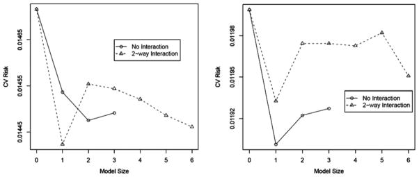
Comparison of cross-validation risk, model size, and model complexity (i.e., interactions) based on DSA-selected MSMs #5 (left) and #8 (right).
Separate results compare estimates of an assumed MSM based on an assumed treatment model (Table 4, model 2) with other assumed MSMs that were based on DSA-selected treatment models (Table 4, models 4 and 7). The differences in the results are indicative of the sensitivity of MSM estimates to the choice of treatment models.
In summary, this analysis demonstrates the utility of the DSA algorithm for selection of treatment models and MSMs that would not likely be considered as potential models in practice. Moreover, it highlights the importance of selection of appropriate treatment models for proper estimation of MSM causal parameters.
10. Discussion
The cross-validation DSA algorithm is one of the first model selection procedures written to identify and to estimate causal models for given data distributions and represents an important advancement in the application of MSMs for epidemiologic research. Development of the algorithm represents the combination of (1) a set of theoretical results that showed that, with cross-validation, an intensive data-adaptive model search can be conducted with finite sample data and that a model, closest in approximation of a true model of the data, can be selected from among many candidate models that might be considered (van der Laan and Dudoit, 2003; van der Laan et al., 2004); and (2) the development of the deletion–substitution–addition (DSA) algorithm used to generate and select models, and, thus, approximate the model space for a given data distribution, based on cross-validation (Sinisi and van der Laan, 2004).
The performance of the algorithm to select models relative to true models of given data was examined with simulations. The algorithm returned consistent models with minimal variance, and returned better representative models of the underlying data than the fixed MSMs that were evaluated. This finding clearly points to the advantages and practical uses of the algorithm with regard to model interpretability and precision. Still, there is the potential for bias, as suggested by the simulation that included increased levels of confounding. Biased IPTW estimates in particular can occur as the result of large subject-specific weights, and reflect a violation of the ETA assumption necessary for the identification of causal effects (Cole and Hernán, 2008). Different methods can be employed to address this assumption (Hernán et al., 2000; Robins et al., 2000; van der Laan and Robins, 2002; Haight et al., 2003; Bembom and van der Laan, 2007). Other estimators are available, too, that can provide consistent and potentially more efficient estimates than IPTW (van der Laan and Robins, 2002; van der Laan and Rubin, 2006; Robins et al., 2007; Tan, 2007; Cao et al., 2009; Goetgeluk et al., 2009).
The real-data analysis provided the opportunity to compare models the algorithm selected with hypothetical assumed models, i.e., a priori models. The treatment models selected by the cross-validation DSA algorithm demonstrated the algorithm’s capacity to identify variables and relationships between those variables that were not originally assumed. Similarly, the algorithm’s selection of an MSM that excluded FEV1 as a causal effect demonstrated the algorithm’s choice of a model that was more representative of the underlying data; i.e., FEV1 in the assumed model was measured with imprecision; therefore, there was no clear evidence that it represented a causal effect with the given data. Although the analysis was oversimplified, it illustrated the use of algorithm to examine and recast the modeling assumptions that are applied in data analyses.
The cross-validation DSA algorithm represents an important methodological advancement with important statistical and subject matter implications for model selection and MSM analyses. It provides for exploration of a wide assortment of possible models, beyond what current forward/selection procedures can explore, and from these obtain a model closest to the true model of the given data. Consequently, one can have greater confidence in the inferences one derives from analyses, given that the models selected do not depend entirely on a priori assumptions (they still depend on chosen variables used in the selection process), but are more likely to represent underlying patterns in data. The algorithm is intended as a tool to augment the search of potential causal mechanisms, but is not expected to replace one’s discretion in terms of one’s knowledge of potential underlying causal mechanisms.
The DSA algorithm has additional functions that were not developed for the cvDSA procedure: (1) selection of models based on different numbers of observations, depending on the number of terms with missing values included in the model search; (2) random partitioning of data into training and validation subsets for cross-validation, rather than generating fixed partitions only; and (3) extension of the machine-learning approach where user-supplied models are assessed with respect to model fit, and if necessary, augmented by the algorithm to provide more reasonable fits of given data. Both the DSA and cvDSA packages are based on an integrated data-adaptive estimation procedure, which enable model searches that are concurrently intensive and robust.
In summary, this paper was intended to illustrate the motivation behind the development of the cross-validation DSA algorithm, examine the mechanisms by which the algorithm selects models, and explore various aspects of the algorithm through simulation and data analysis to inform the researcher who decides to include it among his/her analytical tools.
Supplementary Material
Acknowledgments
The authors wish to express their gratitude to Bianca Kaprielian, for her assistance in the preparation of the manuscript, and Boriana Pratt, for her technical assistance and thoughts with regard to the simulation.
Appendix. Supplementary data
Supplementary data associated with this article can be found, in the online version, at doi:10.1016/j.csda.2010.02.002.
Footnotes
Selection criterion submitted to the DSA algorithm allowed the procedure to select models up to eight terms, with second-order polynomials and 2-way interactions.
Selection criterion submitted to the cvDSA algorithm allowed the procedure to select models up to six terms with 2-way interactions.
References
- Bembom O, van der Laan MJ. A practical illustration of the importance of realistic individualized treatment rules in causal inference. Electronic Journal of Statistics. 2007;1:574–596. doi: 10.1214/07-EJS105. [DOI] [PMC free article] [PubMed] [Google Scholar]
- Bickel P, Doksum K. Mathematical Statistics–Basic Ideas and Selected Topics. Prentice Hall; NJ: 2001. p. 18. [Google Scholar]
- Brookhart MA, van der Laan MJ. A semiparametric model selection criterion with applications to the marginal structural model. Computational Statistics and Data Analysis. 2006;50 (2):475–498. [Google Scholar]
- Bryan J, Yu Z, et al. Analysis of longitudinal marginal structural models. Biostatistics. 2004;5 (3):361–380. doi: 10.1093/biostatistics/5.3.361. [DOI] [PubMed] [Google Scholar]
- Cao W, Tsiatis AA, et al. Improving efficiency and robustness of the doubly robust estimator for a population mean with incomplete data. Biometika. 2009;96:723–734. doi: 10.1093/biomet/asp033. [DOI] [PMC free article] [PubMed] [Google Scholar]
- Cole SR, Hernán MA. Constructing inverse probability weights for marginal structural models. American Journal of Epidemiology. 2008;168 (6):656–664. doi: 10.1093/aje/kwn164. [DOI] [PMC free article] [PubMed] [Google Scholar]
- D’Agostino RB, Lee ML, et al. Relation of pooled logistic regression to time dependent Cox regression analysis: The Framingham heart study. Statistics in Medicine. 1990;9:1501–1515. doi: 10.1002/sim.4780091214. [DOI] [PubMed] [Google Scholar]
- Dudoit S, van der Laan M, et al. Loss-based estimation with cross-validation: Applications to microarray data analysis and motif finding. Department of Biostatistics, University of California; Berkeley, CA: 2003. [Google Scholar]
- Efron B, Tibshirani RJ. An Introduction to the Bootstrap. 45–55. Chapman and Hall; London: 1993. pp. 237–241. [Google Scholar]
- Eisner M, Wang Y, et al. Second-hand smoke exposure, pulmonary function, and cardiovascular mortality. Annals of Epidemiology. 2007;17 (5):364–373. doi: 10.1016/j.annepidem.2006.10.008. [DOI] [PubMed] [Google Scholar]
- Goetgeluk S, Vansteelandt S, et al. Estimation of controlled direct effects. Journal of the Royal Statistical Society: Series B Statistical Methodology. 2009;70 (5):1049–1066. [Google Scholar]
- Haight T, Neugebauer R, et al. Comparison of inverse probability of treatment weighted estimator and a naive estimator. Department of Biostatistics, University of California; Berkeley, CA: 2003. [Google Scholar]
- Hernán M, Brumback B, et al. Marginal structural models to estimate causal effect of zidovudine on the survival of HIV-positive men. Epidemiology. 2000;11 (5):561–570. doi: 10.1097/00001648-200009000-00012. [DOI] [PubMed] [Google Scholar]
- Mortimer KM, Neugebauer R, et al. An application of model-fitting procedures for marginal structural models. American Journal of Epidemiology. 2005;162 (4):382–388. doi: 10.1093/aje/kwi208. [DOI] [PubMed] [Google Scholar]
- Neugebauer R, van der Laan MJ. Nonparametric causal effects based on marginal structural models. Journal of Statistical Planning and Inference. 2003;137:419–434. [Google Scholar]
- Robins JM. Association, causation, and marginal structural models. Synthese. 1999;121:151–179. [Google Scholar]
- Robins JM, Hernán MA, et al. Marginal structural models and causal inference in epidemiology. Epidemiology. 2000;11:550–560. doi: 10.1097/00001648-200009000-00011. [DOI] [PubMed] [Google Scholar]
- Robins J, Sued M, et al. Performance of double-robust estimators when inverse probability weights are highly variable. Statistical Science. 2007;22 (4):544–559. [Google Scholar]
- Satariano WA, Smith J, et al. A census-based design for the recruitment of a community sample of older residents: Efficacy and costs. Annals of Epidemiology. 1998;8:278–282. doi: 10.1016/s1047-2797(97)00235-4. [DOI] [PubMed] [Google Scholar]
- Sinisi S, van der Laan MJ. Loss-based cross-validated deletion/substitution/addition algorithms in estimation. Department of Biostatistics, University of California; Berkeley, CA: 2004. [Google Scholar]
- Tager IB, Swanson A, et al. Reliability of physical performance and self-reported functional measures in the elderly. Journal of Gerontology: Medical Sciences. 1998;53A:M295–M300. doi: 10.1093/gerona/53a.4.m295. [DOI] [PubMed] [Google Scholar]
- Tan Z. Understanding OR, PS, and DR. Statistical Science. 2007;22 (4):560–568. [Google Scholar]
- van der Laan M, Dudoit S. Unified cross-validation methodology for selection among estimators and a general cross-validated adaptive epsilon-net estimator: Finite sample oracle inequalities and examples. Department of Biostatistics, University of California; Berkeley, CA: 2003. [Google Scholar]
- van der Laan M, Dudoit S, et al. The cross-validated adaptive epsilon-net estimator. Department of Biostatistics, University of California; Berkeley, CA: 2004. [Google Scholar]
- van der Laan MJ, Robins J. Unified Methods for Censored Longitudinal Data and Causality. Springer-Verlag; New York: 2002. pp. 311–347. [Google Scholar]
- van der Laan M, Rubin D. Targeted maximum likelihood learning. International Journal of Biostatistics. 2006;2(1) [Google Scholar]
- Wang Y, Bembom O, et al. Data adaptive estimation of the treatment specific mean. Journal of Statistical Planning and Inference. 2004;137:1871–1887. [Google Scholar]
- Yu Z, van der Laan MJ. Construction of Counterfactuals and the G-computation Formula. Department of Biostatistics, University of California; Berkeley, CA: 2002. [Google Scholar]
Associated Data
This section collects any data citations, data availability statements, or supplementary materials included in this article.