Teacher’s Corner: Latent Curve Models and Latent Change Score Models Estimated in R

Abstract

In recent years the use of the Latent Curve Model (LCM) among researchers in social sciences has increased noticeably, probably thanks to contemporary software developments and to the availability of specialized literature. Extensions of the LCM, like the the Latent Change Score Model (LCSM), have also increased in popularity. At the same time, the R statistical language and environment, which is open source and runs on several operating systems, is becoming a leading software for applied statistics. We show how to estimate both the LCM and LCSM with the sem, lavaan, and OpenMx packages of the R software. We also illustrate how to read in, summarize, and plot data prior to analyses. Examples are provided on data previously illustrated by Ferrer, Hamagami, & McArdle, 2004. The data and all scripts used here are available on the first author’s website.

A few years ago Ferrer, Hamagami, and McArdle (2004) illustrated how to estimate the parameters of the Latent Curve Model (LCM) with a number of different software programs, all of which, except two (Mx and R), were and still are commercial. Since then three phenomena of interest have occurred. First, the LCM is now well-known and often applied by many researchers in several disciplines. This phenomenon is intimately associated to the progress many software have made to implement this model. Indeed, several software programs include dedicated functions or plugins that spare the user typing or drawing the single LCM elements. At the same time, several specialized textbooks appeared, further divulging this approach (e.g., Bollen & Curran, 2006; Duncan, Duncan, & Strycker, 2006; Preacher, Wichman, MacCallum, & Briggs, 2008).

The second phenomenon of interest is that the LCM can be conceived as belonging to a more general family of SEM, the Latent Change Score Model (LCSM, McArdle, 2009; McArdle & Nesselroade, 1994; McArdle, 2001). The LCSM has also gained in popularity, albeit to a lesser degree than the LCM, especially in psychology and the social sciences (e.g., Ghisletta, Bickel, & Lövdén, 2006; Gerstorf, Lövdén, Röcke, Smith, & Lindenberger, 2007; King et al., 2006; McArdle, Hamagami, Meredith, & Bradway, 2000; McArdle & Hamagami, 2001; McArdle, Ferrer-Caja, Hamagami, & Woodcock, 2002; McArdle, Grimm, Hamagami, Bowles, & Meredith, 2009; Lövdén, Ghisletta, & Lindenberger, 2005; Raz et al., 2008).

Finally, and much more general, is the wider use of the R language and environment for statistical descriptive and inferential analyses. This software program is free, both in financial terms and in terms of allowing users to change and share its code. R has become a central statistical program among statisticians with advanced computer programming skills and users without advanced technical knowledge in several scientific fields.

In this article we update Ferrer et al. (2004) to discuss how to estimate the LCM with R and some of its new components (packages). We also expand the discussion by focusing on the LCSM. We first remind the reader of the specifications of the LCM and expand upon them to discuss the LCSM. We then very succinctly discuss the R software and its packages for the estimation of SEM. We also show how to read in, prepare, and plot longitudinal data in R. Finally, we estimate a series of LCMs and LCSMs with R with an application to a historical data set. All R scripts used for the preparation of this article and the data can be found on the first author’s website at http://www.unige.ch/fapse/mad/ghisletta/index.html.

Latent Curve Models and Latent Change Score Models

Analysts of longitudinal data have largely benefited from two parallel statistical developments: LCMs on the one hand, for SEM users, and, on the other hand, multilevel, hierarchical, random effects, or mixed effects models, all extensions of the regression model for dependent units of analysis. Although under certain conditions the two approaches are equivalent (McArdle & Hamagami, 1996; Rovine & Molenaar, 2000; Ghisletta & Lindenberger, 2004), we will focus on the SEM framework because this will allow us extending easily our discussion to LCSMs.

The Latent Curve Model

The LCM is a particular kind of SEM applied to repeated-measures (longitudinal) data, where Y has been measured from time t = 0 to t = T on i = 1, …, N individuals (Laird & Ware, 1982; McArdle, 1986; Meredith & Tisak, 1990). The simplest representation of the model presumes that Y is contingent only upon t as in

$$Y_{i,t}={\beta }_{0,i}+{\beta }_{1,i}\times t_{i,t}+{\epsilon }_{i,t}$$ (1)

where ε_i,T is the error component varying in time and across individuals. The underlying assumptions are that

$$\begin{array}{r}{\beta }_{0,i}~N({\gamma }_0,{\tau }_{00})\\ {\beta }_{1,i}~N({\gamma }_1,{\tau }_{11})\\ {\epsilon }_{i,t}~N(0,{\sigma }^2)\end{array}$$ (2)

meaning that β_0,i, β_1,i, and ε_i,t are normally distributed, with mean γ₀, γ₁, and 0 and variance, τ₀₀, τ₁₁ and σ², respectively. Usually the model also allows for the covariance cov(β_0,i, β_1,i) = τ₀₁. This model is especially adequate to data structured on two levels, where repeated measures varying across time t are nested within individuals i.

Under multivariate normality the LCM is equivalent to the multilevel, hierarchical, random effects, and mixed effects models, where the parameters representing sample averages (γ₀ and γ₁) are also called fixed effects, while individual deviations from the sample averages (represented by τ₀₀, τ₁₁, τ₀₁ and σ²) are called random effects.

It is very common in the SEM literature to represent graphically the models with diagrams. We chose to represent the LCM according to the reticular action model (McArdle & McDonald, 1984) as discussed in Boker, McArdle, and Neale (2002). This type of graphical representation allows users to calculate all expectations according to precise tracing rules (Wright, 1920). Squares or rectangles represent manifest (measured) variables, circles or ellipses represent latent (unmeasured) variables, one-headed arrows represent structural weights (regression paths, factor loadings, means, and intercepts; i.e., fixed effects), two-headed arrows represent covariances (which, if defined from and to the same variable are equivalent to variances; i.e., random effects), and the triangle represents a constant of value 1 used to include means and intercept (one-headed arrows emanating from the triangle).

Figure 1 represents a LCM for data assessed repeatedly at four irregularly spaced occasions, times 0, 1, 3, and 5, represented by squares. Consequently, measurements at times 2 and 4 are missing, or latent, thus represented by circles. These node or phantom variables are inserted to show how the change process is supposed regular over equal time intervals. The latent variables B0 and B1 represent β₀ and β₁ in equation (1) and are often called intercept or level and slope or change, respectively. The factor loadings of B0 are fixed at 1 while for B1 they are linearly increasing according to t, as in equation (1). The two fixed effects are the factor means, MB0 and MB1, while the random effects are the factors’ variances and covariance, VB0, VB1, and CB0B1, and the error variance, Ve, represented here invariant over time (other specifications are possible).

Figure 1.

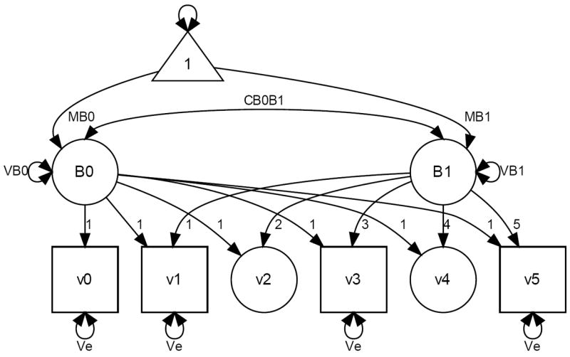
Representation of a Latent Curve Model.

The simple LCM of Figure 1 estimates a total of 6 parameters but obviously less restrictive versions are possible. For instance, the homogeneity of the residual variance assumption can be relaxed to estimate a separate parameter at each occasion (as long as an assessment took place; in Figure 1 this would not be possible at grades 2 and 4). At times it is also sensible to test for auto-regressions in the errors, so that the error variance matrix would not be limited to be diagonal (e.g., Curran & Bollen, 2001). Another popular specification of the LCM consists in freeing the slope loadings, which is equivalent to estimating the change shape that best fits the data. Such a slope is said to have a free (latent) basis (McArdle, 1986). A large variety of change shapes other than linear can also be specified, and many examples of this are available (e.g., Blozis, 2007; Browne, 1993; Curran & Bollen, 2001; Davidian & Giltinan, 1995; Ghisletta & McArdle, 2001; Ghisletta, Kennedy, Rodrigue, Lindenberger, & Raz, 2010; Grimm & Ram, 2009).

The Latent Change Score Model

While in the LCM the focus is on describing a variable Y at time t, in the LCSM we render explicit ΔY_t, the change in Y from t – 1 to t (McArdle & Nesselroade, 1994; McArdle, 2009):

$$Y_{i,t}=Y_{i,t-1}+\mathrm{\Delta }{Y}_{i,t}.$$ (3)

From equation (3) we can easily see that

$$\mathrm{\Delta }{Y}_{i,t}=Y_{i,t}-Y_{i,t-1}.$$ (4)

This basic change in paradigm, classical in time series models (Browne & Nesselroade, 2005; Nesselroade, McArdle, Aggen, & Meyers, 2002), allows, or even forces, the analyst to express the expectation for the change in Y. In this mode we can re-express the LCM in equation (1) by expanding equation (4) as:

$$\mathrm{\Delta }{Y}_{i,t}=({\beta }_{0,i}+{\beta }_{1,i}\times t_{i,t}+{\epsilon }_{i,t})-({\beta }_{0,i}+{\beta }_{1,i}\times t_{i,t-1}+{\epsilon }_{i,t-1})={\beta }_{1,i}\times (t_{i,t}-t_{i,t-1})+{\epsilon }_{i,t}-{\epsilon }_{i,t-1}.$$ (5)

According to equation (5) it then becomes clear that the only influence on the change in Y (ΔY) is the time-invariant slope β₁ (i.e., the B1 factor in Figure 1). Indeed, the residual components have expectations 0 and are usually assumed uncorrelated. Moreover, if the values of t_i,t (corresponding to the loadings of B1 in Figure 1) increase linearly as a function of t, then changes in Y are constant across equal intervals of time (i.e., change is linear).

The expectation of equation (3) can be enhanced by considering also a proportionality effect, besides the slope effect, such that ΔY_i,t = α × β_1,i + β × Y_i,t−1. This yields:

$$Y_{i,t}=Y_{i,t-1}+\alpha \times {\beta }_{1,i}+\beta \times Y_{i,t-1}=\alpha \times {\beta }_{1,i}+(1+\beta )\times Y_{i,t-1}.$$ (6)

Substantively, this corresponds to the frequent hypothesis that the amount of change an individual undergoes is partially proportional to the starting or previous point (through β), partially due to a constant influence (the slope β₁).

Figure 2 represents graphically a LCSM, in which the latent change scores are under the dual influences as in equation (6). To simplify the diagram all unlabelled paths are fixed at 1. Note that to maintain the expectations invariant over equal intervals of time we added again two node variables v2 and v4. To identify the model the α parameter is usually fixed at 1. The diagram clearly conveys the idea that the linear LCM is indeed statistically nested within the LCSM. It suffices to fix α = 1 and β = 0 to simplify equation (6) and obtain

$$Y_{i,t}=Y_{i,t-1}+1\times {\beta }_{1,i}+0\times Y_{i,t-1}=Y_{i,t-1}+{\beta }_{1,i},$$ (7)

which, according to equation (3), is equivalent to

$$\mathrm{\Delta }{Y}_{i,t}=Y_{i,t}-Y_{i,t-1}={\beta }_{1,i}.$$ (8)

Figure 2.

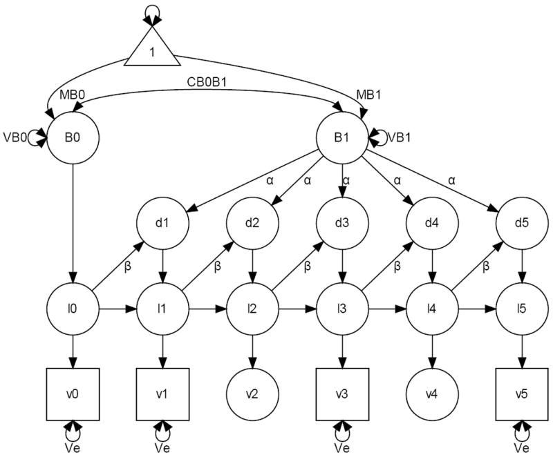
Representation of a Latent Change Score Model.

Illustrative data

To illustrate the estimation of the models in R we rely on the combined data originally published by Osborne and Suddick (1972) and Osborne and Lindsey (1967), also reanalyzed by McArdle and Epstein (1987) and presented by Ferrer et al. (2004). Several (n = 204) pupils were assessed repeatedly (preschool - which we’ll call grade 0 -, grades 1, 3, and 5) on tasks from the Wechsler Intelligence Scale for Children (WISC; Wechsler, 1949). Here we consider the verbal composite score made up of the information, comprehension, similarities, and vocabulary tasks.

To get acquainted with the data we start by examining violin plots, which represent classical boxplots enriched on either side by the data density plots (Hintze & Nelson, 1998). In Figure 3 we can see that the center, the dispersion, and the positive asymmetry of the data increase with grades.

Figure 3.

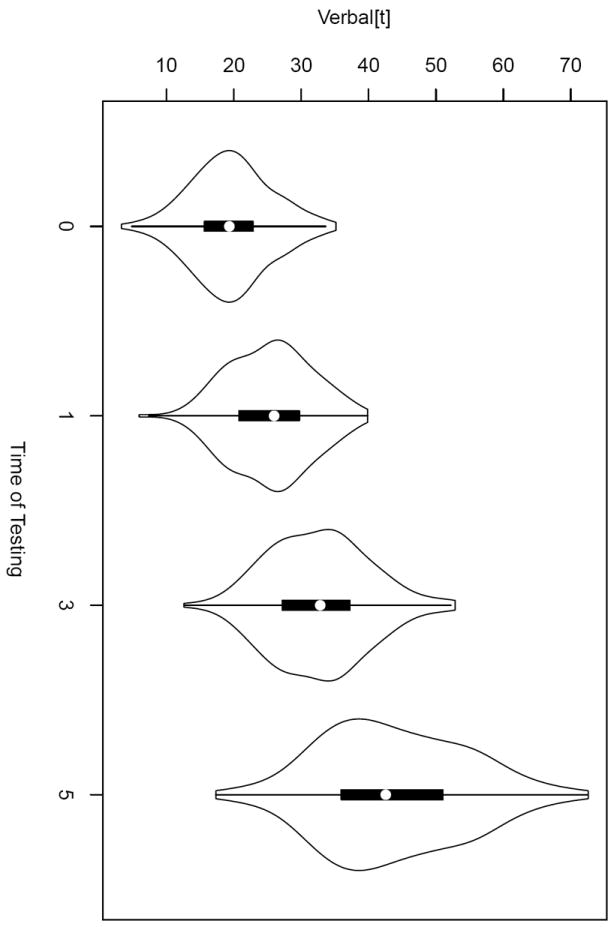
Violin plots of verbal performance scores by time of testing.

Next, we proceed to truly longitudinal plots. To get a closer look at individual change patterns we examine Trellis graphics of 10 randomly selected students, represented in Figure 4. These plots consist in a separate panel for each participant, in which the 4 verbal repeated measures are represented as a function of grade. The empty dots represent the verbal scores as a function of grades and the lines join the points belonging to the same student. Generally we see that scores increase in time and that there is quite some variability in both initial score and in verbal learning rate.

Figure 4.

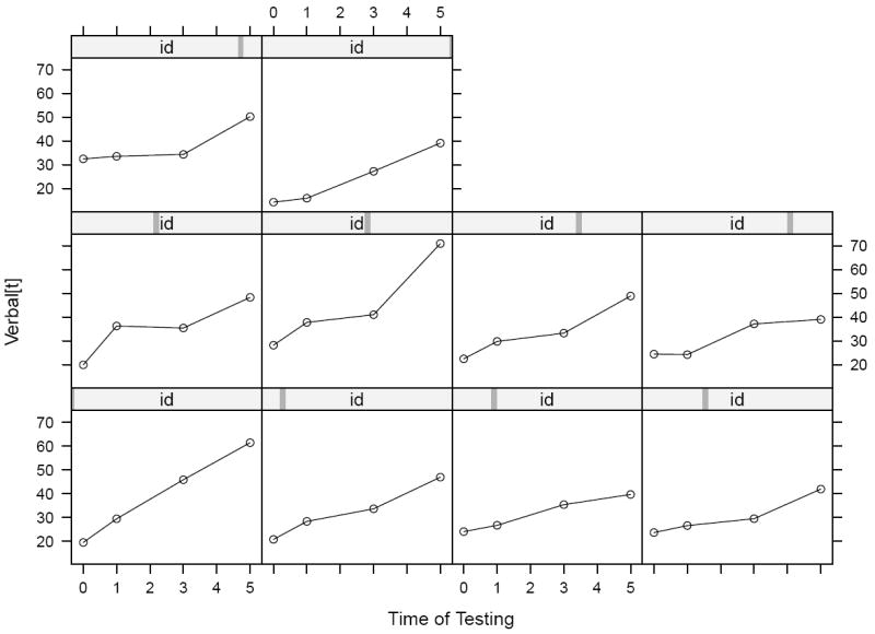
Separate individual trajectories of verbal performance scores by time of testing for 10 randomly chosen individuals.

At times it is more convenient to represent such individual panels overlaid in a single plot, as appears in Figure 5. This plot gives the clear impression that individual students appear to increase in verbal performance as they advance in grade but that there is strong heterogeneity in these trajectories.

Figure 5.

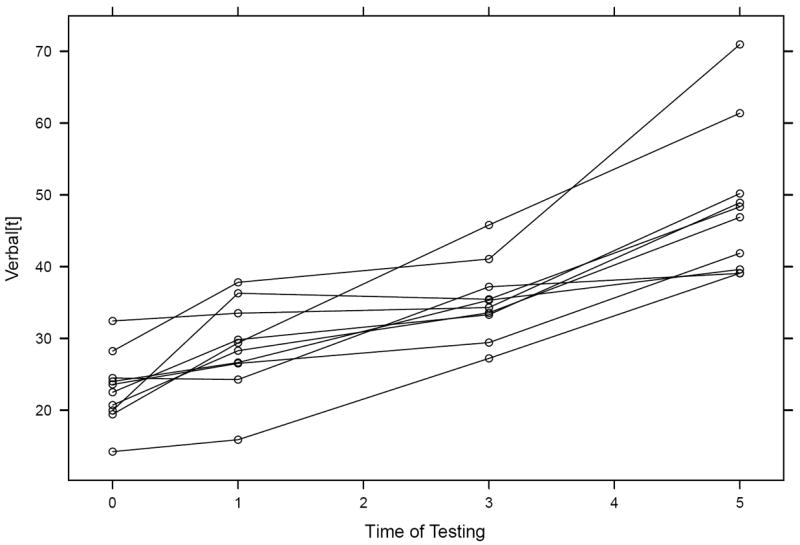
Overlaid individual trajectories of verbal performance scores by time of testing for 10 randomly chosen individuals.

Finally, we also examine typical descriptive statistics. First we notice that for each variable the data set counts 204 observations. There are no cases of missing data. We also see that the scores on the repeated verbal component of the WISC increase in their central tendency (mean, median, and the robust trimmed mean), in their dispersion (standard deviation, range, and the robust median absolute deviation), and also in their deviation from normality (skewness and kurtosis). These classical and robust estimates of central tendency and dispersion were obtained with the psych package in R (Revelle, 2010).

	var	n	mean	sd	median	trimmed	mad	min	max	range	skew	kurtosis	se
verbal0	1	204	19.59	5.81	19.34	19.50	5.41	3.33	35.15	31.82	0.13	−0.05	0.41
verbal1	2	204	25.42	6.11	25.98	25.40	6.57	5.95	39.85	33.90	−0.06	−0.34	0.43
verbal3	3	204	32.61	7.32	32.82	32.42	7.18	12.60	52.84	40.24	0.23	−0.08	0.51
verbal5	4	204	43.75	10.67	42.55	43.46	11.30	17.35	72.59	55.24	0.24	−0.36	0.75

The R language and environment

R (R Development Core Team, 2010; Ihaka & Gentleman, 1996) is a language and environment for statistical computing and graphics based on the S language and environment (Becker & Chambers, 1984; now available in the TIBCO Spotfire S+ program, TIBCO Software Inc., 2010). The source code of R is freely available under the GNU General Public License (GPL) at http://www.r-project.org. Precompiled binaries exist for different versions of Unix, Microsoft Windows, and MAC platforms. R is highly extensible thanks to nearly 3000 freely available libraries, called packages, which represent mainly specialized functions of the R language.

The major advantages of R (thanks mainly to the R Development Core Team) are that it is freely available, extremely dynamic in its development (several statistical analyses can only be computed in R), has excellent graphical capabilities, has a good built-in help system (it suffices to type ?topic when help is sought for a topic), allows for user-written functions (which may then be shared to the general R community), and is object-oriented (elements of operations are created to exist independently and general commands are adapted to the nature of all elements). As a consequence, all packages benefit from these features by attributing complicated portions of syntax to objects. The user’s task is then highly simplified and consists in learning the packages’ objects, without having to worry about the underlying syntax. Although R uses a command line interface, which may discourage some novices from adopting it, there are several good graphical user interfaces available. These greatly facilitate learning the basics of the R language (cf. http://www.sciviews.org/rgui/).

Reading in and manipulating data in R

In this section we explain how we read in and manipulated the data to then obtain the previous graphs and descriptive statistics. Throughout the paper we show R input syntax preceded by the > symbol. Subsequent lines without this symbol represent the output.

R can read in a variety of data formats, whether in common text formats (such as fixed or free format, or as. csv, comma separated values), or coming from well-known closed source statistical software such as SAS, SPSS, Minitab, or SYSTAT. For the former type of data format the user does not need to load a special package, whereas for the latter the foreign package is very useful (Lumley, DebRoy, Bates, Murdoch, & Bivand, 2011). Our data are in free format, in ASCII text with single spaces as delimiter. To read this format we use the read.table function.

The data file name is wisc.dat, missing data are indicated by NA (“not available” in R, although this data set does not contain any missing values), and the first row contains the variables’ names (hence we specify header=TRUE). Note that commands in R are case sensitive so that, for instance, true is not equivalent to TRUE. The result is attributed, with the left-arrow (<-) operator, to a new object we call wisc.

• > wisc <- read.table(“wisc.dat”, na.strings = “NA”, header=TRUE)

To check that the data were read in correctly we use the describe function of the psych package (Revelle, 2010). We first install the psych package with the install.packages command. The dependencies=TRUE option guarantees that if this package necessitates other non installed packages they will also be installed. To limit the output we select the four verbal composite scores. We do so by selecting a subset that we call wisc.verbal of the entire data frame wisc with the operators [ and ]. We retain all rows (hence we do not specify anything before the comma within the square brackets) and select the columns by specifying and combining the names of the four variables (c(“verbal0”, “verbal1”, “verbal3”, “verbal5”)). The output of these commands are the descriptive statistics shown above.

• > wisc.verbal <- wisc[,c(“verbal0”, “verbal1”, “verbal3”, “verbal5”)]

• > install.packages (“psych”, dependencies=TRUE)

• > library(psych)

• > describe(wisc.verbal)

To plot the individual longitudinal data we randomly select 10 participants. We first define a new object that corresponds to the total number of lines (i.e., observations) of the wisc data frame with the nrow() function (which counts the rows of the specified object). We apply again the matrix selection operators [ and ] and the sample() operator, which randomly selects 10 rows (individuals) of the wisc.verbal data frame. At the same time, all columns (corresponding to variables) are selected because nothing is specified after the comma in the square brackets.

• > ntot <- nrow(wisc.verbal)

• > wisc.verbal.sel <- wisc.verbal [sample (ntot, 10),]

To obtain longitudinal plots of the data of these 10 randomly selected individuals we need to reshape their data frame from a so-called large or wide format, where to each occasion of measurement corresponds a variable, to a long format, where the repeated measures of any individuals are piled up to form a vector with multiple rows. The wide format is typically used when estimating SEMs. However, longitudinal plots require the long format. We make use of the reshape function, created for this purpose. We first specify the data frame we want to reshape (wisc.verbal.sel), the names of the variables in the wide format to be reshaped into a single variable in long format (varying=list(c(“verbal0”, “verbal1”, “verbal3”, “ verbal5”))), the name of the variable to be created in long format (v.names= “verbal”), the values of the new variable that differentiates the repeated measures belonging to a given individual (times=c(0,1,3,5)), and finally that we want to reshape to long format (direction= “long”). The resulting reshaped data frame creates the object wisc.verbal.sel.long. The five arguments we specified for this function are separated by commas and, as any series of commands in R, can either be written on a single line or on multiple lines.

• > wisc.verbal.sel.long <- reshape(wisc.verbal.sel,

• > varying=list(c(“verbal0”,“verbal1”,“verbal3”,“verbal5”)),

• > v.names=“verbal”, times=c(0,1,3,5), direction=“long”)

Obtaining longitudinal plots in R

To obtain the violin plots the data must be in wide format. We activate the vioplot package (Adler, 2009) and finally plot the variables by referring to them as elements of the wisc.verbal data frame with the dollar sign $. We label the time points (to avoid the default values of 1,2,3,4) and concatenate these names with the c operator. We require the data density plot to be white (col= “white”). Finally we use the title function simply to label the two axis.

• > install.packages(“vioplot”, dependencies=TRUE)

• > library(vioplot)

• > vioplot(wisc.verbal$verbal0, wisc.verbal$verbal1, wisc.verbal$verbal3, wisc.verbal$verbal5,

• >  col= “white”, names=c(“0”, “1”, “3”, “5”))

• >  title(xlab= “Time of Testing”, ylab= “Verbal[t] ”)

The Trellis graphics can be obtained with the lattice package (Deepayan, 2008, 2011). We ask to plot verbal as a function of time separately for each individual (∣ id) in the wisc.verbal.sel.long data frame. We ask that points and lines joining them be overlaid (type=“o”) and appear in black (col= “black”). We also specify with the xlab and ylab arguments that the labels should not simply be the variables’ names.

• > install.packages(“lattice”, dependencies=TRUE)

• > library(lattice)

• > xyplot(verbal ~ time ∣ id, data = wisc.verbal.sel.long, type=“o”, col=“black”,

• > xlab=“Time of Testing”, ylab=“Verbal[t]”)

To obtain the preceding individual trajectories overlaid within a single panel we use the same function but replace the (∣ id) command by the groups=id argument.

• > xyplot(verbal ~ time, groups=id, data = wisc.verbal.sel.long, type=“o”, col=“black”,

• > xlab=“Time of Testing”, ylab=“Verbal[t]”)

Note that in R all graphs can either be displayed on a panel within the program and then saved as bitmap, metafile or postscript, or outputed directly to external files in different formats (pdf, ps, eps, bmp, wmf, etc.).

Structural Equation Modeling packages in R

Three packages are particularly useful for estimating structural equation models in R: sem, available through the R website, lavaan (for latent variable analysis), available through the R website but also at http://lavaan.ugent.be, and OpenMx, (the R-version of Mx, Neale, Boker, Xie, & Maes, 2006), available at http://openmx.psyc.virginia.edu/.

All three are open source and adapted the R language to estimate a large variety of SEMs. Hence, the three packages are not only appealing because they are open source, but also because they allow to integrate easily their results in the R environment for further operations. They also accept R objects to be integrated in their syntax. sem was developed by John Fox, who maintains it, with contributions from Adam Kramer and Michael Friendly; lavaan is developed and maintained by Yves Rosseel; OpenMx is funded by the National Institute of Health and involves a team of several people: Steve Boker (principal investigator), Michael Neale, Hermine Maes, and Michael Wilde (co-principal investigators), Tim Brick, Jeff Spies, Michael Spiegel, Ryne Eastabrook, Michael Hunter, Sarah Kenny, Paras Mehta, Timothy Bates, John Fox, and Zhiyong Zhang. We provide a succinct discussion of each package only. The interested reader is encouraged to explore the references of each package for further information.

The sem package in R

At the time of writing we use version 0.9-21 (Fox, 2010). Fox described his package in a previous issue of this journal (Fox, 2006; where he also provides a gentle introduction to R). This was the first R package for SEM and it allows estimating parameters of structural equations of manifest variables by two-stage least squares and of general SEMs by maximum likelihood (ML). At the time of writing, the package does not allow to calculate case-wise ML, that is a likelihood function at the individual (raw data), rather than at the group (moment matrix), level. Thus, incomplete data can only be handled either with a multiple group approach by applying ML to each group’s covariance matrix (if the number of patterns is low, see below) or by imputation (several packages to this effect are available in R).

The sem package uses formulation of the reticular action model (RAM ; McArdle, 1980; Boker et al., 2002), which distinguishes three elements of any SEM: a matrix with one-headed arrows (regression weights and factor loadings), a matrix with two-headed arrows (variances and covariances), and a filter matrix, in which manifest and latent variables are distinguished. If means are also included in a model, a sum-of-squares-and-cross-products matrix is to be analyzed instead of a covariance matrix. The package offers a function to this effect. Endogenous and exogenous variables are not distinguished, nor are zero-order from residual variances.

Multigroup analysis is not integrated in the current version of sem. However, if groups are identical in size they can be analyzed within sem by using the stacked models notion, as described by Evermann (2010). Hence, incomplete data in a number of limited patterns can only be dealt with ML estimation if groups are equal in size.

sem produces dot files to generate diagrams in an external program (e.g., GraphViz, an open source graph visualization software available at http://www.graphviz.org/). The dot syntax can be edited to implement changes in appearance. We produced Figures (1) and (2) by editing their dot syntax.

The lavaan package in R

At the time of writing we use version 0.4-7 (Rosseel, 2011). This package is more recent and allows for more options than sem. Three estimators are available for continuous data: ML, generalized least squares, and weighted least squares (also called asymptotic distribution free). Moreover, for ML four methods of estimation of standard errors (SE) are available: the conventional SE based on inverting the (either observed or expected) information matrix, robust SE (with a Satorra-Bentler scaled chi-square statistic), SE based on first-order derivatives, and robust Huber-White SE (with a scaled Yuan-Bentler statistic). lavaan also contains full support for the analyses of means/intercepts and multiple groups. The syntax of lavaan is quite simple and contains a series of popular functions. For instance, dedicated functions are defined for confirmatory factor analyses, latent curve models, several degrees of invariance, etc. Each dedicated functions implements a specific set of default values. There is however also a function that avoids all default values (this is a desirable feature in advanced SEMs). Lastly, the user can ask for the output to appear in Mplus (Muthén & Muthén, 1998-2010) or EQS (Bentler, 1995) format.

At the time of writing, lavaan does not allow for the analyses of categorical or censored variables, mixture models, and multilevel data. According to the author these features should be included in the near future. The lavaan website offers a short description of the package, the minimum R syntax necessary to run a SEM, an example of a simple SEM, but also a very useful tutorial. The package does not produce syntax to draw diagrams. However, the psych package (Revelle, 2010) includes a function to this end.

The OpenMx package in R

This package is described in Boker et al. (in press). At the time of writing we use version 1.0.6-1581 (OpenMx Development Team, 2010). This package is not yet on the R website because of a license restriction on one portion of the code (the NPSOL optimizer, which is not open-source). According to the authors this should be remedied in the near future.

This package is certainly the most complete in R for SEM and this may be due mainly to two reasons. First, OpenMx builds on the already available Mx software, which was a pioneer for several advanced SEM features (Neale et al., 2006). These include the implementation of the ML algorithm at the individual data level (case-wise ML), analyses of non-continuous variables, multilevel analyses, but also the possibility to include any matrix algebra calculation within the model (very powerful feature for nonlinear or any kind of parameter algebraic constraint) and to specify one’s own fitting function (besides the already existing ML and FIML). Indeed, Mx and OpenMx are not just packages for SEM, but more generally for matrix algebra optimization.

The second reason that sets this package apart from the previous two is that, thanks to its funding, OpenMx is maintained by a large and very active team that also created a very rich website with much documentation, several tutorials, didactic presentations, wikis, and forums. Altogether these features allow for immediate feedback to users and make this one of the most complete SEM software available, even when compared to commercial counterparts.

Estimating LCMs in R

The model comparison strategy in SEM, suggested by Jöreskog (1977), is facilitated with statistically nested models (where parameters of the simpler model form a subset of those of a more complex model). In the following we present the syntax to test a fully specified LCM with a linear change function and then discuss how parameter constraints may be imposed to estimate alternative models and compare them to each other.

In the subsequent portions of R syntax we will work with the wisc data frame we have already read in and plotted above. For each package we show how the data can be either analyzed directly or re-expressed appropriately for analyses.

LCMs in the sem package

We start by loading the sem package (library(sem)). The sem package does not implement ML at the individual data level (case-wise ML). To implement ML we need to analyze a moment matrix. The package has a dedicated function that re-expresses raw data so that the variables’ covariance matrix is augmented to include the information about the variables’ means. This is accomplished with the augmented sum-of-squares-and-cross-products (ASSCP) matrix, which can be obtained with the raw.moments function after we activate the package with library(sem). The cbind operator is used to add a column of 1s to the wisc.verbal data frame so that the final ASSCP matrix includes the variables’ means.

• > library(sem)

• > wisc.verbal.mom <- raw.moments(cbind(wisc.verbal, 1))

The final ASSCP matrix is of dimension 5×5 (the 4 verbal scores and the vector of their means, called 1) and is shown below (it su3ces to type the name of the object, wisc.verbal.mom):

• > wisc.verbal.mom

• Raw Moments

• 	verbal0	verbal1	verbal3	verbal5	1
  verbal0	417.13813	523.09980	669.36173	897.1602	19.58505
  verbal1	523.09980	683.04473	862.39082	1159.0913	25.41534
  verbal3	669.36173	862.39082	1116.58309	1488.5354	32.60775
  verbal5	897.16016	1159.09128	1488.53537	2027.2397	43.74990
  1	19.58505	25.41534	32.60775	43.7499	1.00000

• N = 204

To specify the LCM of equation (1) we use the specify.model() command and specify as many lines as parameters (both constrained and estimated) with two kinds of operators. The -> operator indicates structural weights (one-headed arrows), while <-> indicates covariances and variances (two-headed arrows). Unnamed variables that are sources (exogenous or independent) to a given structural weight are latent variables. Hence the intercept and slope are called B0 and B1, respectively. After the specification of each parameter follows either a label, in which case the parameter will be estimated, or NA to attribute a given value to, or fix, the parameter. The last argument of the line is the starting value if the parameter is free or its value if fixed. For instance, the first line below indicates that a latent variable B0 has a loading towards the variable verbal0 (which is manifest because it belongs to the analyzed data set), is fixed (because of NA), and has value 1. Given the restricted structure of the linear LCM all loadings of B0 and B1 are specified likewise.

Next we specify the residual variances (σ² in equation (3)) of the 4 manifest verbal scores. By attributing the same label Ve to the four parameters we constrain them to equality. The two following lines use the special command 1 which indicates means or intercepts. This corresponds to the triangle with the same label in Figure 1. We provided a starting value of 20 to the mean of B0 to facilitate convergence (this value is quite realistic given that it corresponds roughly to mean of verbal0). The last three lines are to include the variances of B0 and B1 as well as their covariance. Importantly, all lines must follow as a sequence because the first empty line within the specify.model() function denotes the end of the specification. Note that at the beginning of this function we attributed the model specification to the object LCM.model with the R attribution operator <-.

• > LCM.model <- specify.model()

• >  B0 -> verbal0, NA, 1

• >  B0 -> verbal1, NA, 1

• >  B0 -> verbal3, NA, 1

• >  B0 -> verbal5, NA, 1

• >  B1 -> verbal0, NA, 0

• >  B1 -> verbal1, NA, 1

• >  B1 -> verbal3, NA, 3

• >  B1 -> verbal5, NA, 5

• >  verbal0 <-> verbal0, Ve, NA

• >  verbal1 <-> verbal1, Ve, NA

• >  verbal3 <-> verbal3, Ve, NA

• >  verbal5 <-> verbal5, Ve, NA

• >  1 -> B0, MB0, 20

• >  1 -> B1, MB1, NA

• >  B0 <-> B0, VB0, NA

• >  B1 <-> B1, VB1, NA

• >  B0 <-> B1, CB0B1, NA

• >

To run the model we use the sem command and specify, in order, the name of the model (LCM.model), the data file (the ASSCP matrix wisc.verbal.mom), and the number of observations of this matrix (we again use the nrow operator to count the observations in the wisc.verbal data frame). The analysis of an ASSCP matrix requires the last two specifications (fixed.x=“1”, raw=TRUE) to adjust automatically the degrees of freedom of the analysis (else it would appear that 5, not 4, variables are analyzed).

• > LCM.fit <- sem(LCM.model, wisc.verbal.mom, nrow(wisc.verbal), fixed.x=“1”, raw=TRUE)

To explore the results we use the generic summary() operator.

• > summary(LCM.fit)

• Model fit to raw moment matrix.

•  Model Chisquare = 79.175 Df = 8 Pr(>Chisq) = 7.161e-14

•  BIC = 36.630

•  Normalized Residuals

  Min.	1st Qu.	Median	Mean	3rd Qu.	Max.
  -0.78300	-0.26800	0.00000	0.00895	0.28400	0.67000

• Parameter Estimates

• 	Estimate Std Error z value Pr(>|z|)
  Ve	12.8278	0.89830	14.2800	0.0000e+00	verbal0 <--> verbal0
  MB0	19.8244	0.36691	54.0313	0.0000e+00	B0 <--- 1
  MB1	4.6734	0.10844	43.0984	0.0000e+00	B1 <--- 1
  VB0	19.8527	2.77131	7.1637	7.8559e-13	B0 <--> B0
  VB1	1.5290	0.24522	6.2353	4.5104e-10	B1 <--> B1
  CB0B1	3.0931	0.58991	5.2433	1.5771e-07	B1 <--> B0

• Iterations = 106

We see that the overall model adjustment is not satisfactory ( ${\chi }_{\mathit{df}=8}^2=79.18$) One immediate reason of misfit in a LCM may reside in the shape of the change function, which we specified to be linear. This is confirmed by the modification indices, which are obtained with the mod.indices() command. Note however that in the sem package the modification indices are based on a preliminary calculation version and are indicative only.

• > mod.indices(LCM.fit)

• 5 largest modification indices, A matrix:

• verbal3:B1	verbal3:verbal5	verbal3:verbal1	verbal3:verbal3	verbal3:B0
  44.07405	44.03124	38.94680	38.38576	38.13363

We see that the biggest modification index for the A matrix is verbal3:B1. In the RAM notation the A matrix concerns the one-headed arrows, or asymmetric effects. This means that there is a substantial gain in statistical fit if the loading from the slope B1 to the indicator verbal3 is estimated rather than fixed at 3. To fully define the latent basis to estimate the shape of change we also free another slope loading, for instance the last, from B1 to verbal5. We do so simply by replacing the NA in the respective lines in the specify.model command by an arbitrary label (i.e., B1 3 and B1 5). The numbers 3 and 5 become now the starting values for these two estimated parameters. Below we show only the two modified lines from the syntax shown above.

• > LCM.free.model <- specify.model()

• >  …

• >  B1 -> verbal3, B1_3, 3

• >  B1 -> verbal5, B1_5, 5

• >  …

We again use the sem () command to run the model and the summary () command to examine the results.

• > LCM.free.fit <- sem(LCM.free.model, wisc.verbal.mom, nrow(wisc.verbal), fixed.x=“1”, raw=TRUE)

• > summary(LCM.free.fit)

• Model fit to raw moment matrix.

•  Model Chisquare = 22.504 Df = 6 Pr(>Chisq) = 0.0009807

•  BIC = -9.4044

•  Normalized Residuals

• Min.	1st Qu.	Median	Mean	3rd Qu.	Max.
  -0.07880	-0.02320	-0.00533	-0.00225	0.02520	0.05080

•  Parameter Estimates

• Estimate Std Error z value Pr(>|z|)
  B1_3	2.2576	0.11102	20.3347	0.0000e+00	verbal3 <--- B1
  B1_5	4.2812	0.21998	19.4620	0.0000e+00	verbal5 <--- B1
  Ve	11.0051	0.77099	14.2740	0.0000e+00	verbal0 <--> verbal0
  MB0	19.7125	0.39418	50.0092	0.0000e+00	B0 <--- 1
  MB1	5.6386	0.33917	16.6246	0.0000e+00	B1 <--- 1
  VB0	20.8299	2.75727	7.5545	4.1966e-14	B0 <--> B0
  VB1	2.4800	0.44807	5.5350	3.1130e-08	B1 <--> B1
  CB0B1	3.2709	0.72199	4.5303	5.8892e-06	B1 <--> B0

• Iterations = 142

The two loadings have an estimated value of 2.26 and 4.28, respectively, which deviate from the previously fixed values of 3 and 5 necessary for a linear basis. Thus, the shape of change deviates from linearity because the yearly gain is no longer fixed at 1 but varies in time. The yearly slope is 1 from grade 0 to 1, 0.63 (=(2.26-1)/(3-1)) from grade 1 to 3, and 1.01 (=(4.28-2.26)/(5-3)) from grade 3 to 5.

To examine whether the loss of the two degrees of freedom resulted in a significant gain in statistical fit we use the anova() function, which compares the statistical fits of two nested models with a likelihood ratio (LR) test.

• > anova(LCM.fit, LCM.free.fit)

• LR Test for Difference Between Models

• 	Model Df	Model Chisq	Df	LR Chisq	Pr(>Chisq)
  Model 1	8	79.175
  Model 2	6	22.504	2	56.67	4.945e-13 ***

We see that we gained 56.67 (=79.17-22.50) χ² points for 2 degrees of freedom, a highly significant improvement in statistical fit (p=4.945e-13). We may hence reject the null hypothesis that the two models are of equal precision.

So far we specified equality of residual variance of the indicators in the LCM. This is however not necessary and this assumption can be relaxed. To do so it suffices to change the labels of the residual variance to be different from each other. The lines below show these modifications:

• > …

• >  verbal0 <-> verbal0, Ve0, NA

• >  verbal1 <-> verbal1, Ve1, NA

• >  verbal3 <-> verbal3, Ve3, NA

• >  verbal5 <-> verbal5, Ve5, NA

• >…

The solution shows a clear improvement in statistical fit. It appears that the residual variance is very similar at grades 0, 1, and 3, but not 5, when its size increases from about 10 to over 25.

• > summary(LCM.freeVe.fit)

• Model fit to raw moment matrix.

•  Model Chisquare = 5.8957 Df = 3 Pr(>Chisq) = 0.11680

•  BIC = -10.059

•  Normalized Residuals

  Min.	1st Qu.	Median	Mean	3rd Qu.	Max.
  -2.48e-02	-4.20e-03	3.66e-03	4.24e-05	6.36e-03	1.86e-02

•  Parameter Estimates

• 	Estimate	Std Error	z value	Pr(>|z|)
  B1_3	2.2585	0.10395	21.7267	0.0000e+00	verbal3 <--- B1
  B1_5	4.2172	0.20899	20.1794	0.0000e+00	verbal5 <--- B1
  Ve0	9.9738	1.64548	6.0613	1.3502e-09	verbal0 <--> verbal0
  Ve1	9.7037	1.30771	7.4203	1.1680e-13	verbal1 <--> verbal1
  Ve3	9.2191	1.51319	6.0925	1.1115e-09	verbal3 <--> verbal3
  Ve5	25.3379	4.31742	5.8687	4.3909e-09	verbal5 <--> verbal5
  MB0	19.6342	0.39105	50.2090	0.0000e+00	B0 <--- 1
  MB1	5.7337	0.32042	17.8943	0.0000e+00	B1 <--- 1
  VB0	21.2545	2.89806	7.3341	2.2338e-13	B0 <--> B0
  VB1	1.6916	0.41450	4.0810	4.4834e-05	B1 <--> B1
  CB0B1	3.5735	0.75281	4.7468	2.0664e-06	B1 <--> B0

The likelihood ratio test confirms the highly significant improvement in statistical fit (over χ² points for 3 degrees of freedom).

• > anova(LCM.free.fit, LCM.freeVe.fit)

• LR Test for Difference Between Models

• 	Model Df	Model Chisq	Df	LR Chisq	Pr(>Chisq)
  Model 1	6	22.5043
  Model 2	3	5.8957	3	16.609	0.0008506 ***

LCMs in the lavaan package

We start by loading the appropriate package with the library(lavaan) command. The procedure is similar to that in sem, where we first specify the model and then submit it for analysis. Because lavaan can compute case-wise ML (i.e., at the individual data level) it accepts data in raw format. To specify the model we write all specifications between single quote marks and then attribute them to an object we call LCM.model.

The B0 and B1 factors are specified with the =~ operator, which means “is manifested as” and specifies one-headed arrows pointing from left to right. The values specified as is preceding an asterisk (*) are fixed. If a latent variable has multiple indicators we can list these on the same line with the plus sign +. Variances are specified with the ~~ operator. Here we set the four variances to equality by using first the label then the equal operator.

• > library(lavaan)

• > LCM.model <- ’ B0 =~ 1*verbal0 + 1*verbal1 + 1*verbal3 + 1*verbal5

• >        B1 =~ 0*verbal0 + 1*verbal1 + 3*verbal3 + 5*verbal5

• >        verbal0 ~~ label(“Ve”)*verbal0

• >        verbal1 ~~ equal(“Ve”)*verbal1

• >        verbal3 ~~ equal(“Ve”)*verbal3

• >        verbal5 ~~ equal(“Ve”)*verbal5’

So far we have not specified which parameters of the latent variables are to be estimated. This is not necessary because we submit the model with the growth command. In this case, by default, lavaan estimates the factors’ means, variances, and their covariance and fixes at zero the indicators’ intercepts. Last we need to specify the data file on which to test the model with the data= command. Note that lavaan selects and utilizes only the manifest variables specified in the model from the data frame. It is hence not necessary to create a smaller data frame containing only the indicators in the model.

• > LCM.fit <- growth(LCM.model, data=wisc)

To explore the results we again use the summary() command. By default the printout of the results contains several goodness of fit indices such as the RMSEA, AIC, BIC, CFI, TLI, and SRMR. For brevity we only report the χ² statistic and the parameter estimates.

• > summary(LCM.fit, fit.measure=TRUE)

• Minimum Function Chi-square			79.175
  Degrees of freedom			8
  P-value			0.0000

• …

• Model estimates:

• 	Estimate	Std.err	Z-value	P(>|z|)
  Latent variables:
  B0 =~
  verbal0	1.000
  verbal1	1.000
  verbal3	1.000
  verbal5	1.000
  B1 =~
  verbal0	0.000
  verbal1	1.000
  verbal3	3.000
  verbal5	5.000
  Latent covariances:
  B0 ~~
  B1	3.093	0.590	5.243	0.000
  Latent means/intercepts:
  B0	19.824	0.367	54.031	0.000
  B1	4.673	0.108	43.098	0.000
  Intercepts:
  verbal0	0.000
  verbal1	0.000
  verbal3	0.000
  verbal5	0.000
  Latent variances:
  B0	19.853	2.771	7.165	0.000
  B1	1.529	0.245	6.236	0.000
  Residual variances:
  verbal0	12.828	0.898	14.283	0.000
  verbal1	12.828
  verbal3	12.828
  verbal5	12.828

We again obtain ${\chi }_{\mathit{df}=8}^2=79.18$. Parameters without standard errors have either been specified as fixed (as the loadings of the latent variables) or constrained to equality (as the residual variances of the indicators). We see that all parameter estimates are equal to those obtained with the sem package.

To obtain modification indices it suffices to add the modindices=TRUE option in the summary() command. By doing so we obtain that the biggest modification index is 45.33 and corresponds to the loading from B1 to verbal3, which is again in favor of estimating the shape of change rather than fixing it to be linear. The modification index of the residual variance of verbal5 is also quite big (23.37), which again speaks against the assumption of homogeneity of residual variance. The latent basis LCM in lavaan is specified by setting free the estimation of the slope loadings to the last two indicators. The free residual variances are specified by applying again different labels for the four parameters and relaxing the equality assumption (not using the label command at all would simply create generic labels in the output). The syntax of the new model is shown below.

• > LCM.freeVe.model <-’ B0 =~ 1*verbal0 + 1*verbal1 + 1*verbal3 + 1*verbal5

• >           B1 =~ 0*verbal0 + 1*verbal1 + start(3)*verbal3 + start(5)*verbal5

• >           verbal0 ~~ label(“Ve0”)*verbal0

• >           verbal1 ~~ label(“Ve1”)*verbal1

• >           verbal3 ~~ label(“Ve3”)*verbal3

• >           verbal5 ~~ label(“Ve5”)*verbal5’

The start() operator specifies a parameter’s starting value. The results are equal to those obtained with the sem package.

LCMs in the OpenMx package

The OpenMx package grants the user a large amount of freedom to explore a very wide variety of general matrix operations and optimization that go beyond the realm of SEM. The simplest way of specifying SEMs is again by using the RAM notation, either by writing the entire matrices in numerical form or by writing only the salient (non-zero) paths. We choose the latter style as we believe it is more intuitive for beginners. First, as usual we load the required package (library(OpenMx)). Then, we create an R object called indic, which consists of the combination (c()) of the names of the indicators (this will shorten the syntax of the models).

• > library(OpenMx)

• > indic <- c(“verbal0”, “verbal1”, “verbal3”, “verbal5”)

The mxModel command serves to specify the model. The first term is a label for the model, the type= defines that we are using the RAM notation, which requires the specification of manifest and latent variables. Then, for each (one-headed or two-headed) path in the diagram depicting the desired model we use the mxPath command. The first specifies the loadings from the intercept to all four indicators, which are one-headed arrows (arrows=1) fixed at one (free=FALSE, values=1). The loadings of the slope are specified analogously. The third mxPath line specifies the residual variances of the indicators, represented by two-headed arrows (arrows=2), which are estimated (free=TRUE), have a starting value of 10 (values=10), and are set to equality because they have the same label (Ve). Next, by specifying a one-headed arrow from the predefined object one to both B0 and B1 we specify the means of the factors, called MB0 and MB1, respectively. We then specify the variances of B0 and B1, with starting values 10 and 1 and labels VB0 and VB1, respectively (else the starting values are 0 and this would render the estimation quite difficult). The covariance between the intercept and the slope follows and is labelled CB0B1. Last, we specify with the mxData command the name of the data file (wisc) and its type. As lavaan did, OpenMx analyzes raw data directly. Note that because we specified the names of the indicators OpenMx, just like lavaan, will select only the indicators of the data frame wisc present in the model.

• > LCM.model <- mxModel(“LCM”, type=“RAM”,

• >   manifestVars=indic,

• >   latentVars=c(“B0”,“B1”),

• >   mxPath(from=“B0”, to=indic, arrows=1, free=FALSE, values=1),

• >   mxPath(from=“B1”, to=indic, arrows=1, free=FALSE, values=c(0,1,3,5)),

• >   mxPath(from=indic, arrows=2, free=TRUE, values=10, labels=“Ve”),

• >   mxPath(from=“one”, to=c(“B0”,“B1”), arrows=1, free=TRUE, labels=c(“MB0”,“MB1”)),

• >   mxPath(from=c(“B0”,“B1”), arrows=2, free=TRUE, values=c(10,1), labels=c(“VB0”,“VB1”)),

• >   mxPath(from=“B0”, to=“B1”, arrows=2, free=TRUE, values=1, labels=“CB0B1”),

• >   mxData(observed=wisc, type=“raw”)

• >   )

Submitting the model simply entails using the mxRun command.

• > LCM.fit <- mxRun(LCM.model)

The summary results contain first some descriptive statistics of the manifest variables, which we omit here. Then we obtain information about the estimated parameters followed by general fit information. Note that because we specified type=raw in the mxData statement the ML algorithm was implemented at the individual level data and, as an indication of the adjustment, we obtain the deviance statistic (-2 log likelihood), which is useful when comparing nested models fitted to the same data. To obtain the χ² value of a model we need to compare its deviance to that of the saturated model (estimating the means of and all variances and covariances among the indicators). The estimation of this latter model does not occur by default. As consequence, OpenMx does not produce by default the deviance of the saturated model (saturated -2 log likelihood: NA). Thus, the χ ² value and degrees of freedom of the specified model, which correspond to the differences between the corresponding deviances and degrees of freedom of the specified and the saturated models, are not reported. Consequently, derived fit indices, such as the RMSEA, are not available by default. This could have been avoided here because the data frame wisc does not have incomplete data. In this case the model tested on the covariance matrix and vector of means of the indicators is equivalent (this is what sem did by fitting the model to the ASSCP matrix). Had we provided the complete data differently to OpenMx we would have obtained the desired statistics.

• > summary(LCM.fit)

• …

• free parameters:

• 	name	matrix	row	col	Estimate	Std.Error
  1	Ve	S	verbal0	verbal0	12.827779	0.8979526
  2	VB0	S	B0	B0	19.852767	2.7708702
  3	CB0B1	S	B0	B1	3.093126	0.5897646
  4	VB1	S	B1	B1	1.529006	0.2450720
  5	MB0	M	1	B0	19.824337	0.3669041
  6	MB1	M	1	B1	4.673384	0.1084349

• observed statistics: 816

• estimated parameters: 6

• degrees of freedom: 810

• -2 log likelihood: 5038.844

• saturated -2 log likelihood: NA

• number of observations: 204

• chi-square: NA

• p: NA

• AIC (Mx): 3418.844

• BIC (Mx): 365.5836

• adjusted BIC:

• RMSEA: NA

To obtain fit statistics we specify and run the saturated model.

• > Sat.model <- mxModel(“Sat”, type=“RAM”,

• >   manifestVars=indic,

• >   mxPath(from=“one”, to=indic, arrows=1, free=TRUE),

• >   mxPath(from=indic, to=indic, all=TRUE, arrows=2, free=TRUE),

• >   mxPath(from=indic, arrows=2, free=TRUE, values=c(30,35,50,115)),

• >   mxData(observed=wisc, type=“raw”)

• >   )

• > Sat.fit <- mxRun(Sat.model)

Finally, we compare the deviance and the degrees of freedom of the saturated model to those of the LCM with the mxCompare function (similar to the anova function used with the sem package). The second line refers to the likelihood ratio test between the saturated and the linear LCM. We again obtain that the linear LCM has a ${\chi }_{\mathit{df}=8}^2=79.17$.

• > mxCompare(Sat.fit, LCM.fit)

• 	base	comparison	ep	minus2LL	df	AIC	diffLL	diffdf	p
  1	Sat	<NA>	14	4959.670	802	3355.670	NA	NA	NA
  2	Sat	LCM	6	5038.844	810	3418.844	79.17452	8	7.166261e-14

OpenMx does not compute modification indices because of the choice of its developers. Indeed, these indices are largely abused of in the literature to obtain theoretically unsubstantiated and non reproducible model specifications, which, of course, are associated to better statistical adjustments. The two modifications to the linear LCM we have implemented above are however quite natural in the context of change. We again (a) estimate the change function by fixing only the first two loadings of the slope factor and (b) relax the homogeneity of residual variance assumption.

In OpenMx a given model is easily updated by simply replacing the new values of the arguments concerned by the modifications. To create the new model LCM.freeVe.model we hence update the previous model by replacing the two slope loadings to be estimated and modifying the labels of the residual variances. The results are identical to those obtained before with sem and lavaan, both in terms of parameter estimation and χ² fit index (we only report these two excerpts from the output).

• > LCM.freeVe.model <- mxModel(LCM.model,

• >  mxPath(from=“B1”, to=c(“verbal3”,“verbal5”), free=TRUE, values=c(3,5), labels=c(“B1_3”,“B1_5”)),

• >  mxPath(from=indic, arrows=2, free=TRUE, labels=c(“Ve0”,“Ve1”,“Ve3”,“Ve5”)))

• > LCM.freeVe.fit <- mxRun(LCM.freeVe.model)

• > summary(LCM.freeVe.fit)

• …

• free parameters

• 	name	matrix	row	col	Estimate	Std.Error
  1	B1_3	A	verbal3	B1	2.258505	0.1037211
  2	B1_5	A	verbal5	B1	4.217229	0.2084919
  3	Ve0	S	verbal0	verbal0	9.973823	1.6433363
  4	Ve1	S	verbal1	verbal1	9.703611	1.3065092
  5	Ve3	S	verbal3	verbal3	9.219143	1.5119445
  6	Ve5	S	verbal5	verbal5	25.337775	4.3137409

• …

• > mxCompare(Sat.fit, LCM.freeVe.fit)

• 	base	comparison	ep	minus2LL	df	AIC	diffLL	diffdf	p
  1	Sat	<NA>	14	4959.670	802	3355.670	NA	NA	NA
  2	Sat	LCM	11	4965.565	805	3355.565	5.895639	3	0.1167995

Estimating LCSMs in R

Below we present the univariate LCSM model tested on the same data as those analyzed with the LCM so far. The univariate specification is particularly well-suited to test whether the deviation from normality detected by estimating the shape of change in the LCM can be mathematically expressed as the proportionality effect β from equation (6). This answers the question whether change is not linear because the latent change score Y_t is not only conditional on a constant effect from the slope β₁ but also on the previous score Y_t−1.

LCSMs in the sem package

A script of the LCSM includes several levels of variables (cf. figure 2). First, the manifest variables are pointed at, with a fixed weight of 1, by latent variables called l0 to l5, which are the true-variance components, free of the residual variance Ve. This is also the case at grade 3 and 5, where no measurement occurred (in that case we point their latent counterparts to an indicator and specify a loading of size 0). Each of these latent variables at time t − 1 influences the next at time t with a fixed weight of 1. Second, the latent change scores d1 to d5 from time t − 1 to time t are defined. These are measured by the corresponding l1 to l5 variables. Moreover, each of these difference scores at time t is influenced by the preceding latent score at time t − 1 through a regression weight labelled beta, for β. The intercept B0 is again anchored at time t = 0 while the slope B1 also influences the latent change scores with a fixed weight of 1 (i.e., α). Last, we specify the mean and variance of both intercept and slope, their covariance, and we set the residual variances of the indicators to equality (Ve).

• > LCSM.model <- specify.model()

• >  l0 -> verbal0, NA, 1

• >  l1 -> verbal1, NA, 1

• >  l2 -> verbal1, NA, 0

• >  l3 -> verbal3, NA, 1

• >  l4 -> verbal3, NA, 0

• >  l5 -> verbal5, NA, 1

• >  l0 -> l1, NA, 1

• >  l1 -> l2, NA, 1

• >  l2 -> l3, NA, 1

• >  l3 -> l4, NA, 1

• >  l4 -> l5, NA, 1

• >  d1 -> l1, NA, 1

• >  d2 -> l2, NA, 1

• >  d3 -> l3, NA, 1

• >  d4 -> l4, NA, 1

• >  d5 -> l5, NA, 1

• >  l0 -> d1, beta, .1

• >  l1 -> d2, beta, .1

• >  l2 -> d3, beta, .1

• >  l3 -> d4, beta, .1

• >  l4 -> d5, beta, .1

• >  B0 -> l0, NA, 1

• >  B1 -> d1, NA, 1

• >  B1 -> d2, NA, 1

• >  B1 -> d3, NA, 1

• >  B1 -> d4, NA, 1

• >  B1 -> d5, NA, 1

• >  1 -> B0, MB0, 20

• >  1 -> B1, MB1, NA

• >  B0 <-> B0, VB0, 20

• >  B1 <-> B1, VB1, 2

• >  B0 <-> B1, CB0B1, 1

• >  verbal0 <-> verbal0, Ve, 5

• >  verbal1 <-> verbal1, Ve, 5

• >  verbal3 <-> verbal3, Ve, 5

• >  verbal5 <-> verbal5, Ve, 5

• >

The results indicate that this model does not provide a good statistical description of the data ( ${\chi }_{\mathit{df}=7}^2=62.13$. The auto-proportion effect β is equal to 0.09 and appears to be significant (the likelihood ratio test comparing this to a nested model with β = 0 results in a ${\chi }_{\mathit{df}=1}^2=17.04$, p < 0.001).

• > summary(LCSM.fit)

• Model fit to raw moment matrix.

•  Model Chisquare = 62.13 Df = 7 Pr(>Chisq) = 5.6616e-11

•  BIC = 24.903

•  Normalized Residuals

• Min.	1st Qu.	Median	Mean	3rd Qu.	Max.
  −0.66700	−0.29600	0.00000	−0.00504	0.28800	0.90800

•  Parameter Estimates

• 	Estimate	Std Error	z value	Pr(>|z|)
  beta	0.090187	0.022535	4.00203	6.2802e-05	d1 <--- l0
  VB0	20.821427	2.783654	7.47989	7.4385e-14	B0 <--> B0
  VB1	0.826091	0.211772	3.90086	9.5852e-05	B1 <--> B1
  CB0B1	0.736818	0.772051	0.95436	3.3990e-01	B1 <--> B0
  MB0	20.338392	0.389351	52.23663	0.0000e+00	B0 <--- 1
  MB1	2.062660	0.654945	3.14936	1.6363e-03	B1 <--- 1
  Ve	12.181386	0.853447	14.27316	0.0000e+00	verbal0 <--> verbal0

• Iterations = 38

Relaxing the homogeneity of residual variance assumption yields to a slight improvement in fit. The resulting likelihood ratio test results in ${\chi }_{\mathit{df}=3}^2=15.70$, p < 0.01. Again, the residual variance at grade 5 is much greater than at the previous grades (results not shown).

LCSMs in the lavaan package

The syntax in lavaan follows the same logic as in sem. Note that we include all estimated parameters in the list defining the model. This is because when we estimate the model we use the lavaan() function, which implements no default values. This is desirable in such an advanced SEM because the LCSM includes a high number of latent variables for which we fix the means and variances to zero rather than estimating them.

• > LCSM.model <- ’ l0 =^~ 1*verbal0

• >        l1 =^~ 1*verbal1

• >        l2 =^~ 0*verbal1

• >        l3 =^~ 1*verbal3

• >        l4 =^~ 0*verbal3

• >        l5 =^~ 1*verbal5

• >        l1 ^~ 1*l0

• >        l2 ^~ 1*l1

• >        l3 ^~ 1*l2

• >        l4 ^~ 1*l3

• >        l5 ^~ 1*l4

• >        d1 =^~ 1*l1

• >        d2 =^~ 1*l2

• >        d3 =^~ 1*l3

• >        d4 =^~ 1*l4

• >        d5 =^~ 1*l5

• >        d1 ^~ label(“beta”)*l0

• >        d2 ^~ equal(“beta”)*l1

• >        d3 ^~ equal(“beta”)*l2

• >        d4 ^~ equal(“beta”)*l3

• >        d5 ^~ equal(“beta”)*l4

• >        B0 =^~ 1*l0

• >        B1 =^~ 1*d1 + 1*d2 + 1*d3 + 1*d4 + 1*d5

• >        B0 ^~ 1

• >        B1 ^~ 1

• >        B0 ^~~ start(20)*B0

• >        B1 ^~~ B1

• >        B0 ^~~ B1

• >        verbal0 ^~~ label(“Ve”)*verbal0

• >        verbal1 ^~~ equal(“Ve”)*verbal1

• >        verbal3 ^~~ equal(“Ve”)*verbal3

• >        verbal5 ^~~ equal(“Ve”)*verbal5’

• > LCSM.fit <- lavaan(LCSM.model, data=wisc)

The results of this first LCSM and of the second, where the residual variances are allowed to vary in size, are identical to those obtained with the sem package.

LCSMs in the OpenMx package

In OpenMx one does not need to allocate a line of syntax to each parameter as in sem or to a class of parameters as in lavaan. This allows the user to set up R objects that may greatly shorten the OpenMx syntax. We do so by first setting up an object indic for the indicators, lat for the latent variables l0 to l5 and diff for the latent change scores d1 to d5.

• > indic <- c(“verbal0”,“verbal1”,“verbal3”,“verbal5”)

• > lat <- c(“l0”,“l1”,“l2”,“l3”,“l4”,“l5”)

• > diff <- c(“d1”,“d2”,“d3”,“d4”,“d5”)

We immediately use these objects to specify the manifest and the latent variables in our LCSM model. We then specify that only 4 elements (lat[c(1,2,4,6)]) of the lat object have one-headed arrows pointing to the indicators. These four elements correspond to the grades at which data were collected (0, 1, 3, 5). The specification of the auto-regressive paths of weight 1 from any latent variable at time t − 1 to the subsequent at time t are greatly simplified by the : operator. For instance, lat[1:5] means elements 1 to 5 of lat. Similarly, we indicate that each latent change score in diff affects the the last 5 variables in lat. Finally, we specify that the first five latent variables in lat affect the latent change scores of diff with a weight labelled beta (hence these five parameters are constrained to equality). The intercept B0 is again anchored on the first latent variable l0 and the slope B1 affects with weight 1 all latent change scores in diff. We specify, label, and provide starting values for the mean of the intercept and slope. Next, we provide starting values for the variances of the intercept, slope, and the residual variances and assign the same label Ve to all residual variances. Last, we specify the covariance between intercept and slope.

• > LCSM.model <- mxModel(“LCSM”, type=“RAM”,

• >    manifestVars=indic,

• >    latentVars=c(“B0”,“B1”,lat,diff),

• >    mxPath(from=lat[c(1,2,4,6)], to=indic, arrows=1, free=FALSE, values=1),

• >    mxPath(from=lat[1:5], to=lat[2:6], arrows=1, free=FALSE, values=1),

• >    mxPath(from=diff, to=lat[2:6], arrows=1, free=FALSE, values=1),

• >    mxPath(from=lat[1:5], to=diff, arrows=1, free=TRUE, values=.1, labels=“beta”),

• >    mxPath(from=“B0”, to=“l0”, arrows=1, free=FALSE, values=1),

• >    mxPath(from=“B1”, to=diff, arrows=1, free=FALSE, values=1),

• >    mxPath(from=“one”, to=c(“B0”,“B1”), free=TRUE, values=c(20,5), labels=c(“MB0”,“MB1”)),

• >    mxPath(from=c(“B0”,“B1”,indic), arrows=2, free=TRUE, values=c(20,2,13,13,13,13),

• >       labels=c(“VB0”,“VB1”,“Ve”,“Ve”,“Ve”,“Ve”)),

• >    mxPath(from=“B0”, to=“B1”, arrows=2, free=TRUE, values=3, labels=“CB0B1”),

• >    mxData(observed=wisc, type=“raw”)

• > )

We can again use the mxCompare command to obtain the likelihood ratio test between this and the saturated model to obtain the overall χ² value and degrees of freedom of this model. To test a second LCSM where we relax the homogeneity of residual variance assumption we can again update the previous model.

• > LCSM.freeVe.model <- mxModel(LCSM.model,(

• >  mxPath(from=c(indic), arrows=2, free=TRUE, values=c(13,13,13,13),

• >  labels=c(“Ve0”,“Ve1”,“Ve3”,“Ve5”))))

The results are again identical to those obtained previously with sem and lavaan.

Discussion

We showed how to estimate basic LCMs and LCSMs with the open source R software. We did not discuss more advanced specifications of the models for space reasons, but extensions to that end of the syntax shown here are straightforward. The purpose was clearly not to provide a full treatment of the sem, lavaan, and OpenMx packages. Interested readers are strongly encouraged to consult the resources cited here.

We have shown that for the models and data presented here the estimated parameters were identical. At this point the question of which package should one use is legitimate. The choice of package should be dictated by several criteria, prime among which are the availability of various SEM features and the difficulty in writing the syntax.

In terms of availability of SEM features, it appears to us that OpenMx is the most complete of three packages discussed here, followed by lavaan. Both offer multigroup analyses and the implementation of the maximum likelihood algorithm at the individual data level, neither of which is available in sem. The specificities of OpenMx are multiple: it allows for categorical threshold estimation, nonlinear inequality constraints, and models with mixed effects. Moreover, OpenMx is written so that models can easily be modified by updating them and further allows for multicore computation. Finally, and beyond SEM, OpenMx is a general matrix optimization package, allowing users to specify their maximization objectives. lavaan provides several estimators and also estimation methods of standard errors. Moreover, the output in lavaan are very user-friendly and contain a rich amount of information.

There is one feature that OpenMx does not provide, and that is modification indices. As discussed before, this was a conscious choice of the developers. Indeed, Browne (2001); MacCallum, Roznowski, and Necowitz (1992) and others have discussed the dangers and the frequent abuses in the SEM literature of modification indices. Although modification indices may be obtained through matrix operations this is clearly not simple for most SEM users. Users absolutely desiring this feature may hence opt for sem or lavaan.

In terms of difficulty in writing the syntax, several users may prefer sem and lavaan, although the mxPath syntax of OpenMx is also quite simple (moreover, the OpenMx team announced the future development of a graphical user interface). This discussion is further complicated when considering the default specifications of each package. Users estimating only LCMs may opt for lavaan, which with its growth function estimates a number of parameters about the level and slope factors by default. However, the presence of default values requires their knowledge by the user, to be sure that all specifications correspond to the desired model to be tested. In our experience, novel users typically ignore what the default values are, while advanced users most often use multiple SEM programs, whose default values are different from one another and hence may create confusion. To avoid all default values one may either use OpenMx or the recent new fitting function lavaan() within the lavaan package.

We remind all users to be cautious and encourage them to check particularly well all parameter specifications of their models in the results. A general advice to this end is to always draw the model first with the complete RAM notation as in Figures 1 and 2. Then count (a) k, the total number of information available in the data (means, variances, and covariances; equivalent to all the parameters estimated in the saturated model) and (b) p, the total number of parameters to be estimated. Finally, compute the degrees of freedom as the df = k − p. In these examples the models included the means, so that based on q, the total number of indicators in the model, df is computed as

$$\mathit{df}=k-p=\frac{q\times (q+3)}{2}-p$$ (9)

Computing the degrees of freedom and checking them for each model is a fundamental skill that should become a reflex for all SEM users.

Last, starting values deserve a separate word. Most SEM software provide by default starting values for any estimated parameter. OpenMx, by default, and lavaan, upon request, do not. Without any default values all parameters to be estimated have a starting value of zero. This can be particularly problematic for variances, which have a lower bound of zero. Users are hence strongly encouraged to specify themselves feasible starting values. This exercise alone forces us to better know both the model and the data and reminds us of the frequent dependency between starting values and final solution.

Conclusion

We have shown how to estimate common and advanced structural equation models about repeated-measures data within the R language and environment. Apart from the obvious advantages of the open source nature of R (gratuity, availability, transparency, flexibility), another major advantage is that SEM analyses can be integrated in a much larger statistical context. Objects created with the SEM packages discussed here can be retrieved and used with any other package (e.g., for further analyses or for plotting). Viceversa, other packages may be used to enhance the SEM analyses. For instance, users not wanting to rely on the missing-at-random or missing-completely-at-random assumption of ML implemented at the individual data level may use dedicated packages for multiple imputation before testing their SEM. In case of simultaneous estimation of independent models specialized packages within R can be applied to distribute the computer jobs over multiple central processing units (CPUs). OpenMx uses the snow and swift packages to this end (Boker et al., in press). Given the richness and availability of specialized packages in R users can create a multitude of synergies between SEM and other packages.

Although we have limited this presentation to univariate instances of LCMs and LCSMs, multivariate extensions are straightforward and often substantively motivated. For instance, within a LCSM applied to two variables measured in parallel it is possible to assess whether one variable is changing not just as a function of that same variable’s previous scores but also as a function of the other variable’s previous scores (McArdle, 2001; McArdle & Hamagami, 2001). Scripts implementing bivariate LCMs and LCSMs on the wisc data presented here are available on the first author’s website.

The authors of R and of the packages discussed here provide an invaluable service to the research community. By sharing their expertise and time (often without compensation) they either implement new or adapt existing descriptive and inferential statistics. The open-source philosophy of R allows anyone with the appropriate skills to modify existing packages and eventually share them with the research community. Users lacking these skills can nevertheless greatly benefit from this shared knowledge. We are extremely glad that both basic and advanced features of SEM have been integrated within the R environment.

References

- Adler D. The ’vioplot’ package in R [Computer software manual] 2009 Available from http://cran.r-project.org/web/packages/vioplot/index.html.
- Becker RA, Chambers JM. S: An interactive environment for data analysis and graphics. Pacific Grove, CA.: Wadsworth and Brooks/Cole; 1984. [Google Scholar]
- Bentler PM. EQS program manual. Encino, C.A.: Multivariate Software, Inc; 1995. [Google Scholar]
- Blozis SA. On fitting nonlinear latent curve models to multiple variables measured longitudinally. Structural Equation Modeling. 2007;14:179–201. [Google Scholar]
- Boker SM, McArdle JJ, Neale M. An algorithm for the hierarchical organization of path diagrams and calculation of components of expected covariance. Structural Equation Modeling. 2002;9:174–194. [Google Scholar]
- Boker SM, Neale M, Maes HH, Wilde M, Spiegel M, Brick T, et al. OpenMx: An open source extended structural equation modeling framework. Psychometrika. doi: 10.1007/s11336-010-9200-6. in press. [DOI] [PMC free article] [PubMed] [Google Scholar]
- Bollen KA, Curran PJ. Latent curve models: A structural equation approach. Hoboken, N.J.: Wiley; 2006. [Google Scholar]
- Browne MW. Structured latent curve models. In: Cuadras CM, Rao CR, editors. Multivariate analysis: Future directions. Vol. 2. Amsterdam, The Netherlands: Elsevier Science Publisher; 1993. pp. 171–197. [Google Scholar]
- Browne MW. An overview of analytic rotation in exporatory factor analysis. Multivariate Behavioral Research. 2001;36:111–150. [Google Scholar]
- Browne MW, Nesselroade JR. Representing psychological processes with dynamic factor models: some promising uses and extensions of autoregressive moving average time series models. In: Madeau A, McArdle JJ, editors. Contemporary advances in psychometrics. Mahwah, NJ.: Erlbaum; 2005. pp. 415–452. [Google Scholar]
- Curran PJ, Bollen KA. The best of both worlds. combining autoregressive and latent curve models. In: Collins LM, Sayer AG, editors. New methods for the analysis of change. Washington, D.C.: American Psychological Association; 2001. pp. 107–135. [Google Scholar]
- Davidian W, Giltinan DM. Nonlinear models for repeated measurement data. London, U.K.: Chapman and Hall; 1995. [Google Scholar]
- Deepayan S. Lattice: Multivariate data visualization with R. New York, NY: Springer; 2008. Available from http://lmdvr.r-forge.r-project.org/ [Google Scholar]
- Deepayan S. The ’lattice’ package in R [Computer software manual] 2011 Available from http://cran.r-project.org/web/packages/lattice/index.html.
- Duncan TE, Duncan SC, Strycker LA. An introduction to latent variable growth curve modeling. 2. New York, N.Y.: Routledge Academic; 2006. [Google Scholar]
- Evermann J. Multiple-group analysis using the sem package in the R system. Structural Equation Modeling. 2010;17:677–702. [Google Scholar]
- Ferrer E, Hamagami F, McArdle JJ. Modeling latent growth curves with incomplete data using different types of structural equation modeling and multilevel software. Structural Equation Modeling. 2004;11:452–483. [Google Scholar]
- Fox J. Structural equation modeling with the sem package in R. Structural Equation Modeling. 2006;13:465–486. [Google Scholar]
- Fox J. The ‘sem’ package in R [Computer software manual] 2010 Available from http://cran.r-project.org/web/packages/sem/index.html.
- Gerstorf D, Lövdén M, Röcke C, Smith J, Lindenberger U. Well-being affects changes in perceptual speed in advanced old age: Longitudinal evidence for a dynamic link. Developmental Psychology. 2007;43:705–718. doi: 10.1037/0012-1649.43.3.705. [DOI] [PubMed] [Google Scholar]
- Ghisletta P, Bickel JF, Lövdén M. Does activity engagement protect against cognitive decline in old age? methodological and analytical considerations. Journal of Gerontology: Psychological Sciences. 2006;61B:P253–P261. doi: 10.1093/geronb/61.5.p253. [DOI] [PubMed] [Google Scholar]
- Ghisletta P, Kennedy KM, Rodrigue KM, Lindenberger U, Raz N. Adult age differences and the role of cognitive resources in perceptual-motor skill acquisition: Application of a multilevel negative exponential model. Journal of Gerontology: Psychological Sciences. 2010;65:163–173. doi: 10.1093/geronb/gbp126. [DOI] [PMC free article] [PubMed] [Google Scholar]
- Ghisletta P, Lindenberger U. Static and dynamic longitudinal structural analyses of cognitive changes in old age. Gerontology. 2004;50:12–16. doi: 10.1159/000074383. [DOI] [PubMed] [Google Scholar]
- Ghisletta P, McArdle JJ. Latent growth curve analyses of the development of height. Structural Equation Modeling. 2001;8:531–555. [Google Scholar]
- Grimm KJ, Ram N. Nonlinear growth models in Mplus and SAS. Structural Equation Modeling. 2009;16:676–701. doi: 10.1080/10705510903206055. [DOI] [PMC free article] [PubMed] [Google Scholar]
- Hintze JL, Nelson RD. Violin plots: a box plot–density trace synergism. The American Statistician. 1998;52:181–184. [Google Scholar]
- Ihaka R, Gentleman R. R: A language for data analysis and graphics. Journal of Computational and Graphical Statistics. 1996;5:299–314. [Google Scholar]
- Jöreskog KG. Structural equation models in the social sciences: Specification, estimation, and testing. In: Krishnaiah PR, editor. Applications of statistics. Amsterdam, The Netherlands: North Holland: 1977. pp. 265–287. [Google Scholar]
- King LA, King DW, McArdle JJ, Saxe GN, Doron-LaMarca S, Orazem RJ. Latent difference score approach to longitudinal trauma research. Journal of Traumatic Stress. 2006;19:771–785. doi: 10.1002/jts.20188. [DOI] [PubMed] [Google Scholar]
- Laird NM, Ware JH. Random-effects models for longitudinal data. Biometrics. 1982;38:963–974. [PubMed] [Google Scholar]
- Lövdén M, Ghisletta P, Lindenberger U. Social participation attenuates decline in perceptual speed in old and very old age. Psychology and Aging. 2005;20:423–434. doi: 10.1037/0882-7974.20.3.423. [DOI] [PubMed] [Google Scholar]
- Lumley T, DebRoy S, Bates D, Murdoch D, Bivand R. The ’foreign’ package in R [Computer software manual] 2011 Available from http://cran.r-project.org/web/packages/foreign/index.html.
- MacCallum RC, Roznowski M, Necowitz LB. Model modifications in covariance structure analysis: The problem of capitalization on chance. Psychological Bulletin. 1992;111:490–504. doi: 10.1037/0033-2909.111.3.490. [DOI] [PubMed] [Google Scholar]
- McArdle JJ. Causal modeling applied to psychonomic systems simulation. Behavior Research Methods and Instrumentation. 1980;12:193–209. [Google Scholar]
- McArdle JJ. Latent growth within behavior genetic models. Behavior Genetics. 1986;16:163–200. doi: 10.1007/BF01065485. [DOI] [PubMed] [Google Scholar]
- McArdle JJ. A latent difference score approach to longitudinal dynamic structural analyses. In: Cudeck R, duToit S, Sorbom D, editors. Structural equation modeling: Present and future. Lincolnwood, IL: Scientific Software International; 2001. pp. 342–380. [Google Scholar]
- McArdle JJ. Latent variable modeling of differences and changes with longitudinal data. Annual Review of Psychology. 2009;60:577–605. doi: 10.1146/annurev.psych.60.110707.163612. [DOI] [PubMed] [Google Scholar]
- McArdle JJ, Epstein DB. Latent growth curves within developmental structural equation models. Child Development. 1987;58:110–133. [PubMed] [Google Scholar]
- McArdle JJ, Ferrer-Caja E, Hamagami F, Woodcock RW. Comparative longitudinal structural analyses of the growth and decline of multiple intellectual abilities over the life span. Developmental Psychology. 2002;38:115–142. [PubMed] [Google Scholar]
- McArdle JJ, Grimm KJ, Hamagami F, Bowles RP, Meredith W. Modeling life-span growth curves of cognition using longitudinal data with multiple samples and changing scales of measurement. Psychological Methods. 2009;14:126–149. doi: 10.1037/a0015857. [DOI] [PMC free article] [PubMed] [Google Scholar]
- McArdle JJ, Hamagami F. Multilevel models from a multiple group structural equation perspective. In: Marcoulides GA, Schumaker RE, editors. Advanced structural equation modeling issues and techniques. Mahwah, NJ: Lawrence Erlbaum Associates; 1996. pp. 89–124. [Google Scholar]
- McArdle JJ, Hamagami F. Latent difference score structural models for linear dynamic analyses with incomplete longitudinal data. In: Collins LM, Sayer M, editors. New methods for the analysis of change. Washington, D.C.: American Psychological Association; 2001. pp. 139–175. [Google Scholar]
- McArdle JJ, Hamagami F, Meredith W, Bradway KP. Modeling the dynamic hypotheses of gf-gc theory using longitudinal life-span data. Learning and Individual Differences. 2000;12:53–79. [Google Scholar]
- McArdle JJ, McDonald RP. Some algebraic properties of the reticular action model for moment structures. British Journal of Mathematical and Statistical Psychology. 1984;27:234–251. doi: 10.1111/j.2044-8317.1984.tb00802.x. [DOI] [PubMed] [Google Scholar]
- McArdle JJ, Nesselroade JR. Using multivariate data to structure developmental change. In: Cohen SH, Reese HW, editors. Life-span developmental psychology: Methodological contributions. Hillsdale, NJ: Lawrence Erlbaum Associates; 1994. pp. 223–267. [Google Scholar]
- Meredith W, Tisak J. Latent curve analysis. Psychometrika. 1990;55:107–122. [Google Scholar]
- Muthén LK, Muthén BO. Mplus user’s guide [Computer software manual] 6. Los Angeles, CA: Muthén and Muthén; 1998-2010. [Google Scholar]
- Neale M, Boker SM, Xie G, Maes HH. Mx: Statistical modeling [Computer software manual] 7. Richmond, VA.: Department of Psychiatry, Virginia Commonwealth University; 2006. [Google Scholar]
- Nesselroade JR, McArdle JJ, Aggen SH, Meyers JM. Alternative dynamic factor models for multivariate time-series analyses. In: Moskowitz DS, Hershberger SL, editors. Modeling intraindividual variability with repeated measures data: Advances and techniques. Mahwah, N.J.: Lawrence Erlbaum Associates; 2002. pp. 235–265. [Google Scholar]
- OpenMx Development Team. OpenMx documentation [Computer software manual] 2010 Available from http://openmx.psyc.virginia.edu/documentation.
- Osborne RT, Lindsey JM. A longitudinal investigation of change in the factorial composition of intelligence with age in young school children. The Journal of Genetic Psychology. 1967;110:49–58. doi: 10.1080/00221325.1967.10533716. [DOI] [PubMed] [Google Scholar]
- Osborne RT, Suddick DE. A longitudinal investigation of the intellectual differentiation hypothesis. The Journal of Genetic Psychology. 1972;121:83–89. [Google Scholar]
- Preacher KJ, Wichman AL, MacCallum RC, Briggs NE. Latent growth curve modeling. Los Angeles, CA: Sage; 2008. [Google Scholar]
- R Development Core Team. R: A language and environment for statistical computing [Computer software manual] Vienna, Austria: 2010. [Google Scholar]
- Raz N, Lindenberger U, Ghisletta P, Rodrigue KM, Kennedy KM, Acker JD. Neuroanatomical correlates of fluid intelligence in healthy adults and persons with vascular risk factors. Cerebral Cortex. 2008;18:718–726. doi: 10.1093/cercor/bhm108. [DOI] [PMC free article] [PubMed] [Google Scholar]
- Revelle W. psych: Procedures for psychological, psychometric, and personality research [Computer software manual] Evanston, Illinois: 2010. Available from http://personality-project.org/r/psych.manual.pdf. [Google Scholar]
- Rosseel Y. The ‘lavaan’ package in R [Computer software manual] 2011 Available from http://cran.r-project.org/web/packages/lavaan/index.html.
- Rovine MJ, Molenaar PCM. A structural modeling approach to a multilevel random coefficients model. Multivariate Behavioral Research. 2000;35:51–88. doi: 10.1207/S15327906MBR3501_3. [DOI] [PubMed] [Google Scholar]
- TIBCO Software Inc. TIBCO Spotfire S+ 8.2 user’s guide. Somerville, MA.: Author; 2010. [Google Scholar]
- Wechsler D. Manual of the wechsler intelligence scale for children. New York, NY.: The Psychological Corporation; 1949. [Google Scholar]
- Wright S. The relative importance of heredity and environment in determining the piebald pattern of guinea-pigs. Proceedings of the National Academy of Sciences. 1920;6:320–332. doi: 10.1073/pnas.6.6.320. [DOI] [PMC free article] [PubMed] [Google Scholar]