Orbital apocenter is not a sufficient condition for HST/STIS detection of Europa’s water vapor aurora

Significance

Images of Europa’s UV aurora taken by the Hubble Space Telescope in December 2012 have revealed local hydrogen and oxygen emissions in intensity ratios that identify the source as electron impact excitation of water molecules. The existence of water vapor plumes as a source for the detected localized water vapor and the possible accessibility of subsurface liquid water reservoirs at these locations have important implications for the exploration of Europa’s potentially habitable environments. The observations reported here tested whether orbital position near the apocenter is an essential requirement for plume activity. Only an upper limit on the amount of water vapor was obtained. Orbital position is therefore not a sufficient condition for detecting plumes and they may be episodic events.

Abstract

We report far-ultraviolet observations of Jupiter’s moon Europa taken by Space Telescope Imaging Spectrograph (STIS) of the Hubble Space Telescope (HST) in January and February 2014 to test the hypothesis that the discovery of a water vapor aurora in December 2012 by local hydrogen (H) and oxygen (O) emissions with the STIS originated from plume activity possibly correlated with Europa’s distance from Jupiter through tidal stress variations. The 2014 observations were scheduled with Europa near the apocenter similar to the orbital position of its previous detection. Tensile stresses on south polar fractures are expected to be highest in this orbital phase, potentially maximizing the probability for plume activity. No local H and O emissions were detected in the new STIS images. In the south polar region where the emission surpluses were observed in 2012, the brightnesses are sufficiently low in the 2014 images to be consistent with any H₂O abundance from (0–5)×10¹⁵ cm⁻². Large high-latitude plumes should have been detectable by the STIS, independent of the observing conditions and geometry. Because electron excitation of water vapor remains the only viable explanation for the 2012 detection, the new observations indicate that although the same orbital position of Europa for plume activity may be a necessary condition, it is not a sufficient condition. However, the December 2012 detection of coincident HI Lyman-α and OI 1304-Å emission surpluses in an ∼200-km high region well separated above Europa’s limb is a firm result and not invalidated by our 2014 STIS observations.

Several lines of evidence point to the existence of a global subsurface water ocean underneath Europa’s icy surface (e.g., refs. 1 and 2), which is speculated to be a habitable environment. Shallow lenses of liquid water may also exist within Europa’s solid crust, causing the formation of disrupted surface features observed at Europa (3). Above Europa’s surface, a tenuous oxygen atmosphere is generated through sputtering by magnetospheric particles (e.g., ref. 4), which has been detected through UV spectra by the Hubble Space Telescope (HST) (5). The ratio of the oxygen emission lines at 1356 Å and 1304 Å of ∼2:1 measured by Hubble is diagnostic of electron impact dissociative excitation of O₂ and the observed brightnesses constrain the O₂ column density to ∼${10}^{14}-{10}^{15}$ cm⁻² (5–8). Results of kinetic modeling of Europa’s hydrogen–oxygen atmosphere (9–12) also find that O₂ is the most abundant component near the surface whereas lighter species like H₂O dominate at higher altitudes. A variable ionosphere has been detected during several measurements by the Galileo spacecraft at different altitudes and geometries (13).

Signs of current geological activity were recently observed at Europa for the first time, when spectral images taken by the HST Space Telescope Imaging Spectrograph (STIS) revealed coincident hydrogen 1216-Å [or Lyman-α (Ly-α)] and oxygen 1304-Å emission surpluses (14). The detected brightnesses and the H to O emission ratio of ∼20:1 are consistent with emission from electron impact dissociative excitation of water vapor with line-of-sight column abundances on the order of 10¹⁶ cm⁻². The spatial extent can be explained by ∼200-km high plumes of water vapor on the anti-Jovian hemisphere near Europa’s south pole (14), presumably originating from effusive or explosive cryovolcanism similar to the plumes on the Saturnian moon Enceladus (e.g., ref. 15). Such cryovolcanic plumes might be fed by subsurface liquid water environments and might thus open a new window to probe these potentially habitable environments (16).

The detected south polar H₂O abundance is presumably transient, as localized H and O emissions were observed only in December 2012, but were not seen during two earlier HST/STIS observation visits in October 1999 and, just one month before the detection, in November 2012 (14). Because Europa was close to its orbital apocenter during the December 2012 detection and closer to its pericenter during the two previous observations, it was proposed (14) that the temporal variability is connected to tidal stresses. Less pronounced putative aurora anomalies detected in previous HST observations have similarly been speculated to originate from plume activity connected to tidal stress effects (8). Polar surface fractures are principally expected to experience tension during the apocenter phase (17), although tension and compression periods depend on the details of the source regions and vary with longitude, latitude, and fault orientation (18). Tensile stresses on fractures possibly drive the opening of faults and subsequent escape of water from the subsurface (14). Cassini recently observed a similar variability of the plumes at Enceladus’s south pole being more active at the orbital apocenter (19, 20).

The existence of water vapor plumes and the possible accessibility of a subsurface liquid reservoir at plume locations have far-reaching implications for the future exploration of Europa’s potentially habitable environment as similarly discussed for Enceladus and its plumes (21, 22). The low spatial resolution and signal-to-noise ratio (SNR) of the STIS images provide only limited information about the detected H₂O abundance, prohibiting accurate constraints on, e.g., the source region or spatial extent.

Two new sets of HST/STIS spectral UV images of Europa near its orbital apocenter were obtained during two HST visits on January 22 and February 2, 2014 to search for water vapor aurora signals to confirm the initial detection and verify the proposed variability pattern (Fig. 1 and Table 1). The January visit was timed to observe Europa at an orbital true anomaly (TA) almost identical to the December 2012 visit (TA centered near 205°), when the water vapor signals were detected. During the February visit Europa was observed at a slightly later orbital position with TA centered around ∼220°. Tidal stress models (14, 18, 23) predict that the tension averaged over all mapped fractures (24) of the south polar region (>55°S latitude) are maximized at this orbital phase. The preplanned true anomaly conditions necessarily also constrained the orbital longitude during the observations in early 2014, such that in both visits the leading anti-Jovian hemisphere was observed (Table 1). Similar to the 2012 visits the 2014 observations were timed to coincide with the maximum variation of Jupiter’s magnetic field orientation. This configuration enables the identification of time-variable aurora inhomogeneities originating from the periodically changing magnetospheric conditions, contrasting them with time-stationary inhomogeneities that potentially are of atmospheric origin (14).

Fig. 1.

Sketch of Europa’s positions in its elliptical orbit during the five observation visits of ∼7-h duration. The new observations cover almost the identical true anomaly range of the initial detection HST visit from December 2012 (not to scale and exaggerated orbit eccentricity).

Table 1.

Parameters of the 2014 HST/STIS observations

Date	Start time, UTC	End time, UTC	Total exposure time, min	Analyzed exposure time*, min	Spatial resolution, km/pixel	Subobserver W longitude, °	System III longitude, °	True anomaly, °
January 22, 2014	14:02	20:53	183	143	76.0	117–146	201–61	191–221
February 2, 2014	08:20	15:07	183	106	77.3	129–157	198–57	208–236
December 30–31, 2012	18:49	01:39	164	164	74.9	79–108	0–218	189†–218

UTC, coordinated universal time.

^*Time of the analyzed portions of the exposures with highest geocoronal background excluded.

^†Value is updated and differs by 4° from the values reported in ref. 14.

In the following section we explain the data processing and extraction of the H and O emission images from the raw spatial–spectral STIS images. Data noise sources and signal-to-noise difficulties that similarly apply to the previous STIS observations (14) are further discussed. We then describe the atmospheric H and O emission and in particular the brightness above the limb of the disk in the new 2014 observations. After this the results of the new 2014 images are discussed in the context of the inferred water vapor signals from December 2012 (14).

Data Processing

Like in the previous three HST/STIS visits to Europa in 1999 and 2012 (14, 25), the moon was observed during five consecutive HST orbits. The STIS was used in first-order spectroscopy mode with the G140L grating and the 52 arcseconds × 2 arcseconds slit, to map the ∼1-arcsecond-wide disk of Europa at wavelengths between 1190 Å and 1720 Å. This mode has been previously used many times to observe the Galilean satellites (e.g., refs. 26–29) and more technical details are explained elsewhere (30). During each of the five orbits per visit two exposures with exposure times of 860 s (orbit 1) and 1,160 s (orbits 2–5) were obtained.

To measure emissions originating from Europa’s neutral environment the spectral images need to be corrected for various other contributions, primarily sunlight both scattered in the foreground geocorona and reflected off the moon’s surface. These two sources are particularly strong at the Ly-α line with brightnesses on the order of tens of kiloRayleighs (kR) (geocorona) and ∼1 kR (surface-reflected light) compared with the measured water vapor signal of ∼600 Rayleighs (R) from December 2012 (14).

The visits took place about 2 mo after Jupiter opposition (January 5) and HST moves from Earth’s dayside to nightside after about one-third of the observing orbit. The geocoronal light that fills the entire slit is therefore particularly strong during the beginning of each orbit (Fig. 2), affecting both the Ly-α and OI 1304-Å lines, except in the first orbit of each visit where the science exposures start later due to initial pointing acquisition.

Fig. 2.

The Ly-α background emission is considerably higher in the first exposures per HST orbit (solid lines) of both the January 22 (blue) and February 2 (red) visits and decreases with time as HST moves into Earth’s shadow. During the second exposures of each HST orbit (dashed lines) the background is more constant and lower.

To optimize the measurement quality we exclude the high-background exposures of orbits 2–5 from the February visit, where the Ly-α background was constantly higher than 10 kR (Fig. 2). The dayside exposures of orbits 2–5 from the January observations are split up in two parts of ∼600 s. Only the second half of the exposures, where the Ly-α background is ∼10 kR or lower, is included in the analysis. Despite this reduction of geocoronal noise, the statistical uncertainties are slightly higher for the 2014 observations due to the reduced total exposure times compared with the December 2012 observations (Table 1).

A background correction is performed along the trace of Europa by subtracting the average count rate in pixels 40–80 rows above and below the disk along the slit. The average subtracted background Ly-α brightnesses of the analyzed low-background subset of exposures are summarized in Table 2. Contributions of solar Ly-α emission back-scattered by neutral hydrogen atoms of the interplanetary medium (IPM) are also subtracted through this step. On the disk of Europa IPM emissions behind the moon are blocked along the line of sight viewed from Earth. A modeled Ly-α contribution from the IPM between Europa and infinity is used to correct this oversubtraction on the disk of Europa, similar to the method previously applied for Io (31). The IPM brightness along the line of sight behind Europa is calculated for the respective observing geometries and based on the daily solar Ly-α flux by a single scattering model (32) (Table 2).

Table 2.

Measured data background, derived FUV albedos, and values of the IPM correction for the 2014 and the December 2012 (detection visit) HST/STIS observations

Date	Average Ly-α background*, kR	FUV Albedo, %†	Integrated solar Ly-α flux‡	Ecliptic longitude§	IPM Ly-α background¶, R
January 22, 2014	4.6	1.7 ± 0.3	4.42×1011 cm−2⋅s−1	103.1	325
February 2, 2014	4.5	1.7 ± 0.3	4.41×1011 cm−2⋅s−1	101.9	306
December 30, 2012	5.1	1.5 ± 0.2	4.12×1011 cm−2⋅s−1	67.7	252

^*Average background away from Europa in the analyzed exposures only (includes geocoronal and IPM Ly-α emissions and detector dark rates).

^†Albedo derived between 1430 Å and 1530 Å. Similar albedo is found at Ly-α (Fig. 3).

^‡Solar flux at 1 AU between 1211 Å and 1221 Å in TIMED/SEE spectra of the observation days (33).

^§Ecliptic longitude of Europa seen from Earth.

^¶IPM Ly-α emissions integrated from Europa to infinity (32). The values have an estimated uncertainty of 20%.

Fig. 3 shows the spectral image of all exposures from the January 22 visit after the subtraction of background emissions. The large majority of the H Ly-α signal originates from surface-reflected sunlight. To eliminate the reflected sunlight, model spectral images are generated by mapping the solar UV spectrum from the day of the observation (33) onto a homogeneously bright disk of Europa. The disk images are convolved with a wavelength-dependent point spread function (PSF) (34) to account for the instrument scattering. By fitting the modeled spectral images to the observed brightness between 1430 Å and 1530 Å a geometric far-ultraviolet (FUV) albedo of 1.7% is measured for both the January (Fig. 3, dotted red line) and February observations. The agreement with the disk-average albedo values derived in the previous STIS (1.4–1.6% with uncertainties of 0.2%) (14), HST Goddard High Resolution Spectrograph (1.3–1.6% with uncertainties of ∼0.5%) (6), and HST Advanced Camera for Surveys observations (1.5%) (8) suggests that no pronounced albedo differences are present between the leading and trailing hemispheres, unlike at longer wavelengths (35, 36). A comparison of the modeled reflected sunlight to the observed brightness around 1216 Å indicates that the albedo also is flat between 1200 Å and 1500 Å. Note that in our previous analysis (14) no correction of the oversubtracted IPM Ly-α emission was applied. This led to an underestimation of the on-disk Ly-α brightness and led to a lower Ly-α albedo. This step has no significant influence on the above-limb plume brightness measurement as the derived lower albedo and thus lower surface reflected contribution cancel out the effect of the oversubtracted IPM. Both contributions (IPM oversubtraction on disk and surface-reflected sunlight) are corrected for by modeling a PSF-convolved signal of Europa’s disk.

Fig. 3.

(Top) Spatial STIS image of the combined exposures from January 22, 2014 after background correction. The arrows point toward Jupiter North (JN) and Jupiter (J). (Bottom) Corresponding integrated spectrum (solid black line with error bars) and modeled spectrum of surface-reflected sunlight (red dotted line).

Previous STIS observations revealed an anticorrelation of the Ly-α morphology to the brightness in visible images (14, 25). On the more contaminated trailing hemisphere, which has a more pronounced brightness dichotomy in the visible imges, Ly-α bright areas were found to coincide with darker visible terrain and vice versa (14). At FUV wavelengths <1500 Å water ice has been shown to have a lower reflectivity than nonice species (37). As a result the brighter Ly-α albedos of the contaminated (visible-darkened) regions could be explained by the surrounding region of purer water ice being relatively darker in the UV. The correlation of Europa’s darker visible areas with UV bright regions is also consistent with the finding that Ganymede’s darker visible surface has a slightly higher FUV albedo (≳2%) than Europa (27).

The brightness variance across the disk of 3 × 3-pixel bins (as displayed in Fig. 4 but before smoothing) is about 50% lower on the leading hemisphere (December 2012 and 2014) than on the trailing hemisphere (1999 and November 2012) and an apparent anticorrelation of the observed Ly-α morphologies to the visible images was not discernable in the new 2014 STIS images (Fig. 4 A–D). Therefore, we have assumed a simple homogeneously bright disk for the surface-reflectance model in the present analysis. However, we note that using inverted visible maps for the UV albedo instead like in a previous analysis (14) yields statistically nearly identical results for the atmospheric emissions. Potential spatial albedo variations imply an uncertainty of the derived atmospheric on-disk emission and we therefore focus on the emissions above the limb, which are affected by surface-reflected light only marginally due to the instrument PSF.

Fig. 4.

(A and B) Visible images of the observed hemispheres with subobserver west longitudes listed and combined STIS images of the 2014 STIS visits. (C and D) Ly-α emission before subtraction of the reflected sunlight. (E–J) Ly-α, OI 1304-Å, and OI] 1356-Å images with reflected sunlight subtracted. STIS pixels are binned 3 × 3, and the images are smoothed to enhance the visibility of the statistically significant features. The dotted light blue circles indicate the multiplet lines. The color scale is normalized to the respective brightness, and the scale maximum (corresponding to 1.0 on the scale) is listed in each image. Oversaturated pixels with intensities above maximum are white. The contours show SNR ratios of the binned pixels and contours for SNR = 1 are omitted in C, D, I, and J.

Aurora Model

To convert the observed aurora brightnesses to neutral gas abundances and to study the significance of the aurora morphology we compare the observations to a simple aurora model. Model aurora images are generated by calculating the expected morphology from an electron-excited atmosphere consisting of O₂, O, and H₂O based on the available cross sections for electron impact (dissociative) excitation of the neutrals (38–41). To be consistent with previous estimations we further apply the constant electron parameters used in previous aurora studies (5–7, 14): a total electron density of 40 cm⁻³, a thermal electron population with a temperature of $T_e=20$ eV, and a suprathermal population with $T_e=250$ eV and a 2% mixing ratio. Contributions from resonantly scattered solar 1304-Å and Ly-α emissions are low (14) and therefore neglected in the present analysis. Continuum absorption will have small effects at the highest H₂O columns in the densest parts of plumes, but is also neglected here.

The standard electron parameters used are based on Voyager measurements (42). Galileo observations revealed time-variable differing plasma sheet conditions (e.g., ref. 43), which are discussed later in Interpretation and Discussion. Note that for higher electron densities than the 40 cm⁻³ assumed here, lower neutral gas column densities would be needed to explain the previously observed signals (e.g., refs. 5, 6, and 14). Similarly, higher neutral gas abundances would be needed in lower electron density regimes, e.g., of ∼30 cm⁻³.

For each spectral line of the oxygen multiplets (1355.6 Å and 1358.5 Å for the OI] 1356-Å doublet and 1302.7 Å, 1304.9 Å, and 1306.0 Å for the OI 1304-Å multiplet) separate images are generated and adjusted to the relative intensities (44). The model disks of each spectral line are superposed with a spatial offset along the rotated dispersion axis. The modeled dispersion of the individual multiplet lines is indicated by blue dotted circles in Fig. 4 G–J.

Observations

H and O Aurora Brightness.

The exposures taken during one visit are combined to increase the signal-to-noise ratio (excluding the exposure time where the geocoronal background is highest; Data Processing). Thereby time-variable aurora morphology features presumably caused by the magnetospheric environment (14) are smoothed over the ∼7-h time span of a visit and potentially eliminated. In contrast, local plume-generated aurora features would be almost spatially fixed as Europa rotates by only ∼30° within the ∼7-h period and should stand out in the combined exposures. The H and O images of the two visits are displayed in Fig. 4.

The aurora morphology of the OI 1304-Å and OI] 1356-Å oxygen emissions is remarkably similar for both visits, with the brightest emissions located around the limb near the leading meridian (Fig. 4 D–J). The similarity of the two oxygen multiplet morphologies indicates common source process and species. The measured ratios of the OI] 1356-Å to the OI 1304-Å aurora brightnesses (Table 3) are somewhat higher than in previous observations and even exceed the ratio of 2 expected for the presumably strongest emission contribution from electron impact excitation of O₂ (6, 14).

Table 3.

Measured atmospheric brightnesses of the 2014 and the December 2012 HST/STIS observations

Date	Total fluxes*				Limb fluxes†
	HI 1216 Å	OI 1304 Å	OI] 1356 Å	O ratio: 135.6/130.4	HI 1216 Å	OI 1304 Å	OI] 1356 Å
January 22, 2014	58 ± 33	25 ± 3	71 ± 3	2.8 ± 0.3	59 ± 33	12 ± 2	39 ± 3
February 2, 2014	66 ± 38	33 ± 3	79 ± 4	2.4 ± 0.3	82 ± 39	18 ± 3	42 ± 4
December 30, 2012‡	47 ± 31	39 ± 3	96 ± 3	2.5 ± 0.2	102 ± 32	21 ± 4	49 ± 3

^*Flux within 1.25 R_E around Europa’s center normalized to $\pi {\mathrm{R}}_{\text{E}}^2$ after subtraction of the reflected sunlight.

^†Average flux between 1 R_E and 1.25 R_E around Europa’s center after subtraction of the reflected sunlight.

^‡Values differ slightly from the values of ref. 14 due to updates in the data processing including the new correction of IPM Ly-α.

The relatively unchanged oxygen aurora morphology between the two visits and the similar measured oxygen brightnesses suggest similar magnetospheric and atmospheric conditions. The latter is not surprising as the visits are only 11 d apart and the geometrical and magnetospheric conditions—given by the subobserver longitudes and the Jovian System III longitudes, respectively (Table 1)—are very similar.

The measured Ly-α brightnesses after subtraction of the reflected sunlight (Table 3) suggest global contributions from an atmospheric source. Global Ly-α emissions can potentially originate from sunlight scattered off atomic hydrogen in the atmosphere, which is likely also the source of the extended Ly-α emissions detected at Ganymede (27, 45). Ganymede’s global Ly-α emissions have peak brightnesses above 500 R and are thus considerably brighter than the global Ly-α brightnesses we find for Europa. Results from similar kinetic models for Europa’s and Ganymede’s atmosphere indicate a similarly higher H abundance at Ganymede with at least four times higher H column densities (figure 3 of ref. 46 and table 2 of ref. 10), which would explain the different global Ly-α brightnesses. Ganymede’s higher surface temperatures compared with those on Europa potentially allow more H to escape before recombining to form H₂ on the surface, leading to the higher H abundance (46). Another potential contribution at Ly-α could be electron impact dissociative excitation of H₂ (47). However, the total Ly-α brightness is highly sensitive to the assumed surface albedo at 1216 Å and for an albedo 10% higher than the derived value (which is within the estimated uncertainty) the remaining brightness is systematically lower by ∼100 R and thus consistent with a zero signal.

In the next section we focus on the Ly-α brightness above the limb and analyze it in context with the observed above-limb oxygen emissions to investigate potential local emission surpluses due to localized water vapor plumes.

Limb Analysis and Aurora Model.

As in our analysis of the previous STIS observations (14), we subdivide the region between 1 R_E (Europa radius) and 1.25 R_E into 18 bins spanning angles of 20° around the disk. Fig. 5A illustrates the analyzed limb bins in the January 2014 Ly-α observation and the corresponding model aurora image. In Fig. 5 B–D the measured limb bin brightnesses (black solid lines) are compared with model results for an atmosphere with and without plumes (dotted lines).

Fig. 5.

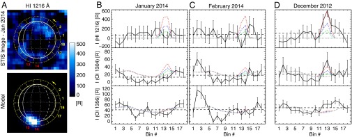
(A) H Ly-α observation image from January 2, 2014 and the corresponding model aurora image including two H₂O plumes derived from the initial detection (14). The 18 analyzed 20° bins around Europa’s disk are shown as yellow dotted lines. The white lines show longitudes and latitudes with the leading meridian (90°W) dashed and the anti-Jovian meridian solid. (B and C) Measured (solid black line) and modeled (dotted lines) brightnesses of the bins for all H and O images from the two 2014 visits. The 2012 plume model atmosphere is shown as dotted red lines. Blue and green dotted lines show a reduced plume density by factors of 2 and 4, respectively. Dashed horizontal lines show average limb brightness. Negative Ly-α limb brightnesses as in the February 2014 bin 14 potentially originate from an oversubtraction of disk-reflected sunlight scattered off the disk through the PSF. (D) December 2012 limb brightnesses for comparison with slightly updated image processing explained in Data Processing and for limb bins defined and shown in figure 3 of ref. 14.

In both 2014 observations, the Ly-α limb brightnesses do not reveal any significant local surpluses above the global average Ly-α brightness discussed in the previous section. The brightest detected Ly-α bins with $217\pm 143$ R in January and $282\pm 167$ R in February exceed the average measured limb brightness (Table 3) by only 1.1σ and 1.3σ, respectively, where σ is the propagated uncertainty of the respective bin (Fig. 5 B and C). A slight enhancement of the OI 1304-Å emission is seen in February in the Ly-α peak bin 15, where the OI] 1356 Å is relatively low as would be expected from electron impact on H₂O, but is also not significant. No other coincident surpluses of the Ly-α and OI 1304-Å emissions are observed. As described in the previous section, the OI 1304-Å morphology is instead very similar to the OI] 1356-Å aurora, suggesting that the O emissions originate from excited O₂.

The observed variation of the oxygen brightnesses around the limb reflects the global oxygen aurora morphology, with the brighter bins located on the leading/sub-Jovian limb. In part, this morphology could originate from the superposed and offset multiplet lines of the OI] 1356-Å and OI 1304-Å emissions. The shifted disks of the fainter lines (dotted blue lines in Fig. 4 G–J) enhance the model brightness on the northern right limb, where the maximum emissions are also found in the data. The model results reveal similar profiles for the bin brightnesses around the limb due to the offset of the multiplet lines, even though the model assumes a symmetric atmosphere and electron environment. The observed variation around the limb might in addition reflect plasma or atmosphere asymmetries that are not in the model. Some brightness variations around the limb exceed the variation of the symmetric model and in particular the bright O emissions in limb bins 2 and 3 in February (Fig. 5C) likely originate from asymmetries in either the electron energy and temperature or the O₂ distribution.

The average OI] 1356-Å limb brightness is consistent with the modeled OI] 1356-Å aurora brightness (Fig. 5 B and C) for the global O₂ atmosphere derived for the previous STIS observations (14) with a radial O₂ column density of $N_{{\text{O}}_2}=3.5\times {10}^{14}$ cm⁻² and a scale height of 150 km. Emissions from electron impact on O and H₂O are insignificant for the expected global abundances (10) and cannot be constrained with the observations. The measured OI 1304-Å brightness is lower than the modeled OI 1304-Å emissions (Fig. 5 B and C, Middle). The reason for this is that for a purely O₂ atmosphere an OI] 1356-Å/OI 1304-Å ratio of ∼2:1 is expected for a Maxwellian temperature distribution around 20 eV as used in our model. The observations revealed a higher ratio. Contributions from excitation of O or H₂O also favor the OI 1304 Å over OI] 1356 Å and thus cannot explain the observed high OI] 1356-Å/OI 1304-Å ratio. Laboratory measurements (40) show that the cross section for electron-impact dissociative excitation of O₂ to the ⁵S° state of O (OI] 1356 Å) is ∼3.3 times higher than the cross section for the ³S° state (OI 1304 Å) for an electron temperature of 16 eV close to the threshold for dissociative excitation of O₂. In the discussed observations (both December 2012 and 2014) Europa’s trailing or wake side was observed, where the electron temperature is decreased through the interaction with Europa’s atmosphere, possibly causing the high OI] 1356-Å/OI 1304-Å ratio.

The colored dotted lines in Fig. 5 B–D indicate the modeled brightnesses for a plume atmosphere based on the December 2012 observations. The plume distribution used is adapted from ref. 14 with two Gaussian-shaped plumes centered at 180°W and at 55°S and 75°S, respectively. For both the January and February observations the brightest Ly-α and OI 1304-Å signal would be expected in limb bin 14 near the south pole, where the detected brightnesses are close to zero.

Interpretation and Discussion

Constraints on Water Vapor Abundance.

No pronounced or coincident Ly-α and OI 1304-Å emission surpluses were detected during two STIS visits in January and February 2014. Assuming a homogeneous electron environment (Aurora Model) and optically thin Ly-α emission from electron impact on H₂O only, the peak measured limb brightnesses of $217\pm 143$ R (January) and $282\pm 167$ R (February) convert to H₂O line-of-sight column densities of $5.0\pm 3.3\times {10}^{15}$ cm⁻² and $6.4\pm 3.8\times {10}^{15}$ cm⁻², respectively. The locations of these brightest bins do not coincide with the south polar region, where the water vapor aurora with Ly-α brightnesses of more than 600 R was detected in 2012. The measured 2014 peak bin brightnesses at Ly-α also do not significantly exceed the average Ly-α limb emissions (Table 3) that might originate from an extended hydrogen cloud around Europa. As explained earlier, the total atmospheric Ly-α brightness, however, strongly depends on the derived surface albedo and is therefore not significant. Other than in the (two) brightest limb bin(s) in January (February) the measured Ly-α limb brightness is below 200 R, implying an upper limit of ∼$5\times {10}^{15}$ cm⁻² for the H₂O column abundance.

The detected water vapor aurora signals from December 2012 were located on the anti-Jovian hemisphere near the south pole. Aurora signals from the same source would be found in almost the same region as the viewing geometry of the new visits differs by only ∼37° (January) and ∼49° (February) with respect to the 2012 detection visit. In particular, the location of the brightest signal detected in December 2012 would barely be affected by the viewing geometry due to its location at high latitude (∼75°S). The Ly-α emissions in the bins, where the brightest plume signal is expected after the model for the December 2012 detection (bins 13 and 14, Fig. 5 A–C), are, however, particularly low and consistent with a zero brightness during both 2014 visits. The brightness in model aurora images generated for the plume atmosphere as derived from the initial detection (Fig. 5D) suggests that Ly-α aurora brightnesses of ∼500 R were to be expected for both visits, assuming that the plume density and electron excitation did not change. The model results indicate upper limits in the 2012 plume region of $3\times {10}^{15}$ cm⁻², i.e., that the plume signal needs to be reduced by at least a factor of ∼4 compared with the 2012 detection, to be consistent with the measured brightnesses in limb bins 13 and 14.

Note that for our simple model plumes an above-limb Ly-α aurora signal of at least 400 R is expected to be always observed from Earth independent of the subobserver longitude due to the high altitude and high-latitude location of the plumes rising above the limb (again assuming the same electron parameters). In other words, the plume aurora should principally be observable, at least in part, from any viewing perspective. In reality the plume gas is more likely ejected from multiple vents along individual linea features and/or enhancements near the intersections of linea (14, 48) and might resemble the gas outflows observed at Enceladus. The observed line-of-sight column density thus potentially varies with viewing perspective as it depends on the alignment of the active vent locations. Lower line-of-sight columns in 2014 could have potentially affected a detection or at least cannot be excluded without further information. The limited spatial resolution of the plume imaging from December 2012 and the uncertainty of the plume source locations, however, prevent further constraints on the plume gas distribution.

Other effects on the detected Ly-α brightness from a plume such as absorption of the IPM Ly-α background by the H₂O plume gas or absorption of plume Ly-α emission by the IPM atomic hydrogen are negligible. The cross section for photoabsorption of Ly-α by H₂O is $\sigma \approx 1.5\times {10}^{-17}$ cm² (49) and the optical depth for the derived average plume column density of $1.5\times {10}^{16}$ cm⁻² (14) is thus $\tau \approx 0.2$. A potential attenuation of the ∼300-R IPM Ly-α background (Table 2) is therefore negligible compared with the 2012 emission brightness of 600 R. The optical depth due to scattering of Ly-α by the interplanetary hydrogen between Jupiter and Earth can approach values of $\tau \sim 0.1$, when Jupiter is at ecliptic longitudes near the IPM upstream direction of $\lambda \approx 252°$ (50, 51). However, during all five previous STIS visits Europa was less than 40° from the IPM downstream direction (see ecliptic longitudes in Table 2), implying very low IPM optical depths. Also, the absorption line center is shifted due to the relative velocity of the IPM H of ∼20 km s⁻¹. If the viewing direction is roughly aligned with the IPM flow, the line shift of ∼0.09 Å is higher than the line width of the electron-excited emission from H₂O of 0.069 Å for an electron temperature of 25 eV (41) and H Ly-α absorption will be even lower.

The nondetection of water vapor aurora in general and in particular of aurora signals from the locations of the initial detection in December 2012 can best be explained by a decreased H₂O abundance, or a decreased electron energy input flux to excite the emissions, or a combination of both. We first discuss the influence of the electron environment, before we elaborate on the potential variability of water vapor sources.

Influence of the Plasma Environment.

Nondetections of water vapor-related aurora signals can in principle originate from a reduced flux of energetic electrons compared with the December 2012 observation leading to emissions below the observational thresholds of the HST/STIS observations. In our aurora calculations we assume a constant homogeneous plasma environment and the aurora brightness is proportional to the ambient torus electron density and also electron temperature through the temperature-dependent excitation rates. We discuss the influence of the varying plasma conditions and focus on the electron density, which scales linearly with brightness in our model. Variations of the thermal electron temperature will also affect the brightness, but are less well constrained by Galileo measurements and therefore not separately discussed here. We further neglect the influence of the interaction of the magnetospheric plasma with the moon atmosphere, which leads to a nonlinear response of the aurora brightness to plasma density variations due to the cooling and deflection of the incoming plasma as shown for Io on the global scale (52) or locally in a plume (53).

Due to the tilt of Jupiter’s magnetic moment with respect to its rotation axis, the magnetic field equator and the centrifugal equator are tilted by ∼9° and ∼6° with respect to the satellite orbital plane (54). The latitudinal density distribution in the plasma sheet is often approximated by an exponential profile that is independent of the local time and symmetric with respect to the centrifugal equator:

$$n\left(z_c\right)=n_0{e}^{-{\left(z_c/H_c\right)}^2}$$ [1]

(equation 2 in ref. 55). Here, $n_0$ is the density in the plasma sheet center, $z_c$ is Europa’s distance above/below the center, and $H_c$ is a scale height of the latitudinal extension around the center. The fast rotation of the inclined Jovian magnetosphere therefore causes periodic variations of the ambient electron density at Europa within the 11.2-h synodic rotation of Jupiter. Based on various Voyager and Galileo measurements, a plasma sheet density distribution from 6 R_J (Jupiter radius) outward was derived (56), which yields $n_0=53$ cm⁻³ and $H_c=1.7$ R_J in Europa’s orbit (9.4 R_J). Taking these values, the plasma density at Europa after Eq. 1 varies only weakly over a full Jovian System III cycle (dashed line in Fig. 6) and is similar to the electron density of 40 cm⁻³ assumed in our aurora model.

Fig. 6.

(Top) Ambient torus plasma and electron densities as a function of the Jovian System III longitude in Europa’s orbit after the model of Bagenal and Delamere (56) (dashed line) and as derived from Galileo PWS measurements (57) (orange triangles). Most of the variation between the Galileo flybys is in accordance with periodic variations from Europa’s changing position with respect to the plasma sheet center (solid line). (Bottom) The System III longitude ranges of the analyzed exposures of the HST visits (2014 and December 2012) are shown in color. For more information see text.

Some of the Galileo plasma density measurements showed higher values near Europa’s orbit (figure 1 of ref. 56). Similarly, measurements by the Galileo Plasma Wave Spectrometer (PWS) during Europa flybys yielded considerably higher electron densities (57). The values shown in Fig. 6 are taken from figure 5 of ref. 57 for times at or before closest approach when the plasma density appears to be undisturbed by the interaction with Europa. The exceptionally high density measured for flyby E12 of more than 600 cm⁻³ is off the vertical range and this case is discussed at the end of this section. The density of the displayed flybys varies roughly by a factor of 4 and most of the values are well in agreement with the periodic variation originating from Europa’s changing position after Eq. 1 in the plasma sheet for a peak density of $n_0=200$ cm⁻³ and a scale height of $H_c=0.9$ R_J (sold line in Fig. 6). This profile is similar to the density profile derived by Schilling et al. (section 3.16 in ref. 58) based on the density range given in table 21.1 of ref. 43. Besides the high density measured during flyby E12, the PWS value from flyby E11 notably differs from the estimated periodic variation by a factor of ∼2.

Like the 2012 observations the new 2014 observations intentionally covered the maximum variation of Jovian magnetic field orientation and the correlated ambient plasma density with the limited set of 5 HST orbits per visit. With the symmetric plasma density distribution described above these magnetospheric conditions imply similar transitions through varying plasma density environments for the 2012 and 2014 visits, with low plasma density at the beginning of each visit and increasing until Europa crosses the plasma sheet center and then decreasing during the second half of the visit (Fig. 6, Bottom). The exposures of the visits in 2012 and 2014 similarly cover the periodic density variations, which therefore very likely cannot cause the brightness difference of ∼600 R (December 2012) compared with 9 ± 137 R (January 2014) and 30 ± 164 R (February 2014) in the plume limb bin (bin 14).

We can also make an estimation about the electron excitation potential, using the oxygen aurora. With the assumption that the global atmospheric O₂ density is identical or very similar during the 2012 and 2014 observations we can use the OI] 1356-Å brightness measured in the south polar region as diagnostic for the relative strength of the electron excitation. The OI] 1356-Å emission originates in large part from electron impact on O₂ and is less affected by local H₂O plumes, mostly indirectly through the interaction of the incoming plasma with the neutral gas obstacle. We further assume that the excitation of the atmospheric O₂ and the plume H₂O occur in roughly the same region along the line of sight and that the brightnesses of the observed O₂ and H₂O emissions are linearly correlated (neglecting, for example, the differing profiles of the temperature-dependent excitation cross sections). Then, a change in brightness of the OI] 1356-Å aurora due to changes in the electron energy flux would lead to the same change of the H₂O aurora brightness for unchanged neutral gas abundances. Note that this approach accounts for changes of both electron density and temperature by estimating the electron energy flux.

The average OI] 1356-Å brightnesses of the south polar limb bins (bins 13–15) during the 2014 visits are 29 ± 5 R and 29 ± 8 R. During the December 2012 visit a roughly two times higher average brightness of 66 ± 7 R was observed in the same bins. This brightness difference could, for example, be connected to a deviation from the average density of factor 2 as seen during flyby E11 (Fig. 6). Thus, for an unchanged H₂O column abundance we would expect that the plume aurora brightness is approximately two times lower in the 2014 observations compared with the detection due to an decreased electron energy flux in the south polar plume region. Because the Ly-α brightnesses detected in 2014 are lower by more than a factor of 4, this estimate with its underlying assumptions suggests that the lower electron energy input cannot entirely account for the nondetection of the anti-Jovian south polar water vapor plumes in the new observations alone. Taking a two times lower electron input flux derived here, the south polar H₂O plume column density detected in December 2012 must still be reduced by at least a factor of 2 during the 2014 visits (compared with a decrease by a factor of 4 for an unchanged electron environment).

On the other hand, a significant plasma and electron density variation independent from the periodic variability like the high density during Galileo flyby E12 will affect the global O₂ atmosphere and potentially also the plume detectability. Whereas the source of Europa’s atmosphere is sputtering of the surface ice by mostly suprathermal ions and therefore relatively independent of the thermal plasma density (4), the dominating atmospheric loss processes—thermal ion sputtering of the atmosphere and electron impact ionization—are proportional to thermal torus electron and ion densities (7). Contributions to atmospheric loss from photoionization are considered to be less important (29). The lifetime of O₂ in Europa’s atmosphere is about 1.5 d (10) and longer than the periodic plasma density variations discussed above. When the thermal plasma density is exceptionally high (low) over a long time period (several hours), the atmospheric O₂ abundance will be lower (higher) and cannot be assumed constant anymore. In this case the OI] 1356-Å brightness cannot be used as a diagnostic for the electron impact. The higher atmospheric loss rate and therefore less dense global atmosphere caused by a high plasma density would lead to a weaker interaction of plasma with Europa’s atmosphere and a lower deflection of the incoming plasma flow (7, 52). This in turn would allow the incoming electrons to reach near-surface regions and favor the excitation of atmosphere and plume gas and thus the detection of a plume. In contrast, a low plasma density could lead to a denser O₂ atmosphere deflecting and cooling the incoming plasma and preventing the excitation of near-surface water vapor.

The comparison of the Ly-α plume brightness variation during the December 2012 detection visit (figure S3 in ref. 14) and the derived periodic density variations (6) also indicate a nonlinear brightness–density correlation. The brightest plume emissions have been detected during the fourth HST orbit between System III longitudes 140° and 170°, whereas the electron density supposedly peaks around a System III longitude of 110° in the third HST orbit. A clear brightness trend outside the uncertainties can, however, not be derived.

Finally, we note that the OI] 1356-Å aurora, which originates mostly from the global O₂ atmosphere, is overall brighter near the poles and fainter in the equatorial region in most images. If this is due to lower electron excitation and not lower O₂ abundance, aurora from H₂O plumes near the equator would likely also be weaker and undetectable in the observed H and O emissions.

Variability of Water Vapor Abundance.

Based on the three HST/STIS observations from 1999 and 2012, Roth et al. (14) proposed a tidally controlled H₂O plume activity that peaks after Europa’s apocenter position where the tensile stresses near the south pole are highest. During the new observations Europa was at orbital true anomalies, (i) which were almost identical to the initial detection (January 2014) and (ii) where tensile stresses in the south polar region maximize (February 2014) (Fig. 1). If the electron environment were not substantially different during the 2012 and 2014 visits, the 2014 nondetections indicate that potential plume activity changes are not governed by a purely periodic variation connected to Europa’s orbital positions or are not periodic at all. The activity might be more episodic like geysers and volcanos on Earth or Io (59) with individual eruptions of unknown frequencies and long periods of dormancy. For Enceladus’s plumes, activity variations by about a factor of 2–3 have been found in addition to the periodic variability (19).

Besides the diurnal radial and librational tides on Europa, which originate from the varying distance and direction of Jupiter as seen from a point on Europa’s surface, additional effects will likely cause tidal stress variations with periodicities differing from the 3.55-d orbital period. Also, Europa is expected to experience long-period obliquity variations (60) and long-period librations (61) due to interactions with neighboring satellites. Both of these effects will give rise to slowly varying stress changes superimposed on the diurnal stress variations.

Impact-Generated Plume.

The total H₂O mass contained within the vapor plume detected in 2012 (14) is about $3\times {10}^6$ kg. The lifetime of ballistic particles launched to a height of 200 km on Europa is only ∼10³ s, much shorter than the duration of the Hubble observations of roughly 7 h. We therefore consider it unlikely that a single impact could have produced the observed long-lived vapor cloud, but for completeness we investigate this possibility below.

Impactor scaling studies (62) provide a method for calculating the mass of vapor produced by an impactor traveling at a specified velocity u. Taking $u=26$ km s⁻¹ (the average impact velocity at Europa according to table 1 of ref. 63), figure 8 of ref. 62 shows that the mass ratio of the vapor to the impactor is about 20, so that the impactor mass in our case needs to be about $1.5\times {10}^5$ kg. Taking a density of 800 kg⋅m⁻³ for consistency with ref. 63, the corresponding impactor diameter d is 7 m. An impactor with diameter $d\ge 1$ km has a probability of striking Europa of $7.0\times {10}^{-7}$ y⁻¹ (table 1 of ref. 63). Although the size-frequency distribution of impactors as small as 7 m is essentially unknown (63), assume that for larger objects the number distribution function follows a power law with $d^{1.97}$. For a 7-m diameter object the corresponding impact probability is then $1.2\times {10}^{-2}$ y⁻¹. In other words, one single 7-m impactor is likely to strike Europa over a time period of 80 y. This result renders the possibility that Hubble fortuitously observed such an event unlikely, but not altogether impossible.

For an impact event on Europa to explain the water vapor plume observed for a duration of ∼7 h an ongoing source of water vapor production by sublimation from a heated surface provides an additional possibility to consider. The LCROSS spacecraft impact event provides a recent example of what is considered to be an ∼10 times larger-than-average lunar impact in the modern era (64). Lunar Reconnaissance Orbiter (LRO)’s Diviner thermal radiometer instrument measured a 30- to 200-m² surface region heated to ∼1,000 K at 90 s postimpact for the ∼20-m diameter crater formed within the Cabeus region by the LCROSS experiment (65). The LCROSS Shepherding Spacecraft NIR2 (Near-IR camera) and Diviner solar channel measurements of blackbody emissions at 250 s postimpact limit the surface temperature to ∼410 K, indicative of a rapid cooling for even lunar regolith and rock material by radiative loss to space. In the two subsequent passes by LRO in its 116-min polar orbit an ∼100-K thermal anomaly was barely present at +2 h and no longer detectable at +4 h.

To compare the lunar case with an impact on the icy surface of Europa we note that the emissivity of lunar regolith (∼0.95) is similar to that of water ice (∼0.98), leaving vertical conduction and porosity the main parameters to consider for relative differences in the timescale for radiative cooling. For the case of Europa’s icy surface, additional cooling by the latent heat of sublimation will decrease the relative timescale. To sustain the ∼3,000 kg⋅s⁻¹ source process maintaining the 10¹⁶ cm⁻² column densities observed over the ∼7-h duration (i.e., an ∼3-h half-life timescale) requires an energy source for sublimation of $2\times {10}^{13}$ J (∼5 kT of TNT), which in this case again requires an equally rare impactor of size 7 m in diameter as described above. Accounting for the energy lost to both the initial ejection of plume material and subsequent radiative cooling and sublimation in this timescale necessitates an even larger initial impactor energy. Hence for this process to be plausible the coincidental observation by HST of an even more unlikely event than the one in 80 y event rate must be invoked.

Summary and Conclusions

We report HST/STIS observations of Europa’s auroral HI 1216-Å (Ly-α), OI 1304-Å, and OI] 1356-Å emissions, which were taken in January and February 2014 with the purpose of confirming the presence of water vapor aurora near the moon’s south pole inferred from previous STIS observations (14). Similar to the 2012 detection visit Europa was near orbital apocenter during the two 2014 HST visits, where tensile stresses in the south polar region are high, potentially increasing the probability of plume activity. With an additional image-processing step compared with that in ref. 14 that takes into account background Ly-α emission from the IPM we show that Europa’s surface albedo does not change significantly between the FUV wavelengths ∼1200 Å and ∼1500 Å.

The new observations did not reveal any pronounced or coincident Ly-α and OI 1304-Å emission surpluses that could be diagnostic for local water vapor abundance through plume activity. The measured brightnesses near the south pole where the plumes were detected in 2012 suggest that no detectable water vapor is present in this region during the 2014 visits. Compared with the December 2012 detection of an ∼600-R Ly-α signal the upper limits of the anti-Jovian south polar 2014 Ly-α brightnesses imply a reduced signal of at least a factor of 4 (Fig. 5 B–D). We also derive a conservative upper limit for the H₂O column density for all locations above the limb of Europa of $5\times {10}^{15}$ cm⁻². The Ly-α brightness in the region of the previous water vapor detection is particularly low (≤50 R) and consistent with zero signal during both visits.

Our simple plume aurora model in contrast suggests that a Ly-α brightness of at least 400 R should be observable above the limb, if a high-altitude high-density plume like that inferred from the December 2012 observation is present in 2014 and the plasma environment did not change considerably. As a check, a Ly-α signal from Europa is not considerably attenuated by the foreground IPM hydrogen column. By using the OI] 1356-Å aurora brightness at the south polar limb, which is barely affected by emissions from dissociated H₂O, as diagnostic for the local electron energy input, we estimate that the electron energy (density and temperature) is lower by a factor of ∼2 during the 2014 visits compared with the 2012 detection. This estimate suggests that the variability of the plasma environment alone cannot explain the nondetection in 2014, and the previously detected water vapor column must also be lower by at least a factor of 2 as well. However, significant aperiodic changes in the electron environment like those observed during Galileo flyby E12 could potentially affect both the O₂ atmosphere and the plume detectability. In this case the OI] 1356-Å brightness cannot be used as proxy for the electron input and such exceptional electron conditions could enable or prevent water vapor detections.

The only viable explanation for the statistically significant and coincident H Ly-α and OI 1304-Å emission surpluses in an ∼200-km high region well separated above Europa’s limb detected in December 2012 (14) remains electron excitation of localized water vapor. If the electron environment was not significantly altered, the nondetections during the 2014 HST visits indicate that the south polar water vapor observed in December 2012 is not equally present at the same orbital true anomaly phases. Activity variations of plumes might be affected by a secondary tidal effect such as long-period librations or obliquity variations or just be nonperiodic and more episodic like geysers and volcanos on Earth or Io. The derived upper limit on the H₂O abundance, however, does not exclude smaller and less dense plumes at any location.

References

- 1.Carr MH, et al. Evidence for a subsurface ocean on Europa. Nature. 1998;391(6665):363–365. doi: 10.1038/34857. [DOI] [PubMed] [Google Scholar]
- 2.Khurana KK, et al. Induced magnetic fields as evidence for subsurface oceans in Europa and Callisto. Nature. 1998;395(6704):777–780. doi: 10.1038/27394. [DOI] [PubMed] [Google Scholar]
- 3.Schmidt BE, Blankenship DD, Patterson GW, Schenk PM. Active formation of ‘chaos terrain’ over shallow subsurface water on Europa. Nature. 2011;479(7374):502–505. doi: 10.1038/nature10608. [DOI] [PubMed] [Google Scholar]
- 4.Johnson RE, et al. In: Jupiter. The Planet, Satellites and Magnetosphere. Bagenal F, Dowling TE, McKinnon WB, editors. Cambridge Univ Press; Cambridge, UK: 2004. pp. 485–512. [Google Scholar]
- 5.Hall DT, Strobel DF, Feldman PD, McGrath MA, Weaver HA. Detection of an oxygen atmosphere on Jupiter’s moon Europa. Nature. 1995;373(6516):677–681. doi: 10.1038/373677a0. [DOI] [PubMed] [Google Scholar]
- 6.Hall DT, Feldman PD, McGrath MA, Strobel DF. The far-ultraviolet oxygen airglow of Europa and Ganymede. Astrophys J. 1998;499:475–481. [Google Scholar]
- 7.Saur J, Strobel DF, Neubauer FM. Interaction of the Jovian magnetosphere with Europa: Constraints on the neutral atmosphere. J Geophys Res. 1998;103:19947–19962. [Google Scholar]
- 8.Saur J, et al. Hubble Space Telescope/Advanced Camera for Surveys observations of Europa’s atmospheric ultraviolet emission at eastern elongation. Astrophys J. 2011;738:153. [Google Scholar]
- 9.Shematovich VI, Johnson RE, Cooper JF, Wong MC. Surface-bounded atmosphere of Europa. Icarus. 2005;173:480–498. [Google Scholar]
- 10.Smyth WH, Marconi ML. Europa’s atmosphere, gas tori, and magnetospheric implications. Icarus. 2006;181:510–526. [Google Scholar]
- 11.Plainaki C, et al. The role of sputtering and radiolysis in the generation of Europa exosphere. Icarus. 2012;218:956–966. [Google Scholar]
- 12.Plainaki C, et al. Exospheric O2 densities at Europa during different orbital phases. Planet Space Sci. 2013;88:42–52. [Google Scholar]
- 13.Kliore AJ, Hinson DP, Flasar FM, Nagy AF, Cravens TE. The ionosphere of Europa from Galileo radio occultations. Science. 1997;277(5324):355–358. doi: 10.1126/science.277.5324.355. [DOI] [PubMed] [Google Scholar]
- 14.Roth L, et al. Transient water vapor at Europa’s south pole. Science. 2014;343(6167):171–174. doi: 10.1126/science.1247051. [DOI] [PubMed] [Google Scholar]
- 15.Porco CC, et al. Cassini observes the active south pole of Enceladus. Science. 2006;311(5766):1393–1401. doi: 10.1126/science.1123013. [DOI] [PubMed] [Google Scholar]
- 16.Spencer JR. Planetary science. Glimpsing eruptions on Europa. Science. 2014;343(6167):148–149. doi: 10.1126/science.1248879. [DOI] [PubMed] [Google Scholar]
- 17.Hurford TA, Helfenstein P, Hoppa GV, Greenberg R, Bills BG. Eruptions arising from tidally controlled periodic openings of rifts on Enceladus. Nature. 2007;447(7142):292–294. doi: 10.1038/nature05821. [DOI] [PubMed] [Google Scholar]
- 18.Nimmo F, Spencer JR, Pappalardo RT, Mullen ME. Shear heating as the origin of the plumes and heat flux on Enceladus. Nature. 2007;447(7142):289–291. doi: 10.1038/nature05783. [DOI] [PubMed] [Google Scholar]
- 19.Hedman MM, et al. An observed correlation between plume activity and tidal stresses on Enceladus. Nature. 2013;500(7461):182–184. doi: 10.1038/nature12371. [DOI] [PubMed] [Google Scholar]
- 20.Nimmo F, Porco C, Mitchell C. Tidally modulated eruptions on Enceladus: Cassini ISS observations and models. Astrophys J. 2014;148:1–14. [Google Scholar]
- 21.Spencer JR, Nimmo F. Enceladus: An active ice world in the Saturn system. Annu Rev Earth Planet Sci. 2013;41:693–717. [Google Scholar]
- 22.McKay CP, Anbar AD, Porco C, Tsou P. Follow the plume: The habitability of Enceladus. Astrobiology. 2014;14(4):352–355. doi: 10.1089/ast.2014.1158. [DOI] [PubMed] [Google Scholar]
- 23.Nimmo F, Thomas PC, Pappalardo RT, Moore WB. The global shape of Europa: Constraints on lateral shell thickness variations. Icarus. 2007;191:183–192. [Google Scholar]
- 24.Selvans ZA. 2009. Time, tides, and tectonics on icy satellites. PhD thesis (University of Colorado, Boulder, CO)
- 25.McGrath MA, Hansen CJ, Hendrix AR. 2009. Observations of Europa's tenuous atmosphere. Europa, eds Pappalardo RT, McKinnon WB, Khurana KK (Univ of Arizona Press, Tucson, AZ), pp 485–505.
- 26.Roesler FL, et al. Far-ultraviolet imaging spectroscopy of Io’s atmosphere with HST/STIS. Science. 1999;283(5400):353–357. doi: 10.1126/science.283.5400.353. [DOI] [PubMed] [Google Scholar]
- 27.Feldman PD, et al. HST/STIS ultraviolet imaging of polar aurora on Ganymede. Astrophys J. 2000;535:1085–1090. [Google Scholar]
- 28.Strobel DF, Saur J, Feldman PD, McGrath MA. Hubble Space Telescope Space Telescope Imaging Spectrograph search for an atmosphere on Callisto: A Jovian unipolar inductor. Astrophys J. 2002;581:L51–L54. [Google Scholar]
- 29.McGrath MA, Lellouch E, Strobel DF, Feldman PD, Johnson RE. In: Jupiter. The Planet, Satellites and Magnetosphere. Bagenal F, Dowling TE, McKinnon WB, editors. Cambridge Univ Press; Cambridge, UK: 2004. pp. 457–483. [Google Scholar]
- 30.Roth L, Saur J, Retherford KD, Feldman PD, Strobel DF. A phenomenological model of Io’s UV aurora based on HST/STIS observations. Icarus. 2014;228:386–406. [Google Scholar]
- 31.Feaga LM, McGrath M, Feldman PD. Io’s dayside SO2 atmosphere. Icarus. 2009;201:570–584. [Google Scholar]
- 32.Pryor WR, et al. In: Cross-Calibration of Far UV Spectra of Solar System Objects and the Heliosphere. Quémerais E, Snow M, Bonnet R-M, editors. Springer; Berlin: 2013. [Google Scholar]
- 33.Woods TN, et al. Solar EUV Experiment (SEE): Mission overview and first results. J Geophys Res. 2005;110:1312. [Google Scholar]
- 34.Krist JE, Hook RN, Stoehr F. 20 years of Hubble Space Telescope optical modeling using Tiny Tim. In: Kahan MA, editor. Optical Modeling and Performance Predictions V. Vol 8127. SPIE; Bellingham, WA: 2011. pp. 1–16. [Google Scholar]
- 35.Nelson RM, et al. Spectral geometric albedos of the Galilean satellites from 0.24 to 0.34 micrometers - Observations with the International Ultraviolet Explorer. Icarus. 1987;72:358–380. [Google Scholar]
- 36.Hendrix AR, Barth CA, Hord CW, Lane AL. Europa: Disk-resolved ultraviolet measurements using the Galileo Ultraviolet Spectrometer. Icarus. 1998;135:79–94. [Google Scholar]
- 37.Hendrix AR, Hansen CJ. Ultraviolet observations of Phoebe from the Cassini UVIS. Icarus. 2008;193:323–333. [Google Scholar]
- 38.Doering JP, Gulcicek EE. Absolute differential and integral electron excitation cross sections for atomic oxygen. VII - The 3P-1D and 3P-1S transitions from 4.0 to 30 eV. J Geophys Res. 1989;94:1541–1546. [Google Scholar]
- 39.Doering JP, Gulcicek EE. Absolute differential and integral electron excitation cross sections for atomic oxygen. VIII - The 3P-5S0 transition (1356 Å) from 13.9 to 30 eV. J Geophys Res. 1989;94:2733–2736. [Google Scholar]
- 40.Kanik I, et al. Electron impact dissociative excitation of O2: 2. Absolute emission cross sections of the OI(130.4 nm) and OI(135.6 nm) lines. J Geophys Res. 2003;108:5126. [Google Scholar]
- 41.Makarov OP, et al. Kinetic energy distributions and line profile measurements of dissociation products of water upon electron impact. J Geophys Res. 2004;109:9303. [Google Scholar]
- 42.Sittler EC, Strobel DF. Io plasma torus electrons - Voyager 1. J Geophys Res. 1987;92:5741–5762. [Google Scholar]
- 43.Kivelson MG, et al. In: Jupiter. The Planet, Satellites and Magnetosphere. Bagenal F, Dowling TE, McKinnon WB, editors. Cambridge Univ Press; Cambridge, UK: 2004. pp. 513–536. [Google Scholar]
- 44.Morton DC. Atomic data for resonance absorption lines. I - Wavelengths longward of the Lyman limit. Astrophys J. 1991;149(Suppl 77):119–202. [Google Scholar]
- 45.Barth CA, et al. Galileo ultraviolet spectrometer observations of atomic hydrogen in the atmosphere at Ganymede. Geophys Res Lett. 1997;24:2147–2150. [Google Scholar]
- 46.Marconi ML. A kinetic model of Ganymede’s atmosphere. Icarus. 2007;190:155–174. [Google Scholar]
- 47.Ajello JM, James GK, Shemansky DE. Cross sections for production of H(2p, 2s, 1s) by electron collisional dissociation of H2. Astrophys J. 1991;371:422–431. [Google Scholar]
- 48.Dombard AJ, Patterson GW, Lederer AP, Prockter LM. Flanking fractures and the formation of double ridges on Europa. Icarus. 2013;223:74–81. [Google Scholar]
- 49.Sander SP, et al. 2011. Chemical Kinetics and Photochemical Data for Use in Atmospheric Studies, Evaluation Number 17 (Jet Propulsion Laboratory, California Institute of Technology, Pasadena, CA)
- 50.Wu FM, Judge DL. Modification of solar lines propagating through the interplanetary medium. J Geophys Res. 1979;84:979–982. [Google Scholar]
- 51.Izmodenov VV. Local interstellar parameters as they are inferred from analysis of observations inside the heliosphere. Space Sci Rev. 2009;143:139–150. [Google Scholar]
- 52.Saur J, Strobel DF. Relative contributions of sublimation and volcanoes to Io’s atmosphere inferred from its plasma interaction during solar eclipse. Icarus. 2004;171:411–420. [Google Scholar]
- 53.Roth L, Saur J, Retherford KD, Strobel DF, Spencer JR. Simulation of Io’s auroral emission: Constraints on the atmosphere in eclipse. Icarus. 2011;214:495–509. [Google Scholar]
- 54.Khurana KK, et al. In: Jupiter. The Planet, Satellites and Magnetosphere. Bagenal F, Dowling TE, McKinnon WB, editors. Cambridge Univ Press; Cambridge, UK: 2004. pp. 593–616. [Google Scholar]
- 55.Hill TW, Michel FC. Heavy ions from the Galilean satellites and the centrifugal distortion of the Jovian magnetosphere. J Geophys Res. 1976;81:4561–4565. [Google Scholar]
- 56.Bagenal F, Delamere PA. Flow of mass and energy in the magnetospheres of Jupiter and Saturn. J Geophys Res. 2011;116:5209. [Google Scholar]
- 57.Kurth WS, et al. The plasma wave environment of Europa. Planet Space Sci. 2001;49:345–363. [Google Scholar]
- 58.Schilling N, Neubauer FM, Saur J. Time-varying interaction of Europa with the Jovian magnetosphere: Constraints on the conductivity of Europa’s subsurface ocean. Icarus. 2007;192:41–55. [Google Scholar]
- 59.Williams DA, Howell RR. In: Io After Galileo: A New View of Jupiter’s Volcanic Moon. Lopes RMC, Spencer JR, editors. Springer Praxis Books/Geophysical Sciences; Berlin: 2007. pp. 133–161. [Google Scholar]
- 60.Bills BG. Free and forced obliquities of the Galilean satellites of Jupiter. Icarus. 2005;175:233–247. [Google Scholar]
- 61.Rambaux N, van Hoolst T, Karatekin Ö. Librational response of Europa, Ganymede, and Callisto with an ocean for a non-Keplerian orbit. Astron Astrophys. 2011;527:A118. [Google Scholar]
- 62.Kraus RG, Senft LE, Stewart ST. Impacts onto H2O ice: Scaling laws for melting, vaporization, excavation, and final crater size. Icarus. 2011;214:724–738. [Google Scholar]
- 63.Zahnle K, Schenk P, Levison H, Dones L. Cratering rates in the outer Solar System. Icarus. 2003;163:263–289. [Google Scholar]
- 64.Colaprete A, et al. Detection of water in the LCROSS ejecta plume. Science. 2010;330(6003):463–468. doi: 10.1126/science.1186986. [DOI] [PubMed] [Google Scholar]
- 65.Hayne PO, et al. Diviner Lunar Radiometer observations of the LCROSS impact. Science. 2010;330(6003):477–479. doi: 10.1126/science.1197135. [DOI] [PubMed] [Google Scholar]