On some generalized discrete logistic maps

Abstract

Recently, conventional logistic maps have been used in different vital applications like modeling and security. However, unfortunately the conventional logistic maps can tolerate only one changeable parameter. In this paper, three different generalized logistic maps are introduced with arbitrary powers which can be reduced to the conventional logistic map. The added parameter (arbitrary power) increases the degree of freedom of each map and gives us a versatile response that can fit many applications. Therefore, the conventional logistic map is considered only a special case from each proposed map. This new parameter increases the flexibility of the system, and illustrates the performance of the conventional system within any required neighborhood. Many cases will be illustrated showing the effect of the arbitrary power and the equation parameter on the number of equilibrium points, their locations, stability conditions, and bifurcation diagrams up to the chaotic behavior.

Introduction

Since 1930 until now iterated maps are still considered very important in the modeling and processing of many fields such as in population biology, encryption, communication and business cycle theory [1–11]. One of the most famous maps comes from the so called continuous logistic equation which was introduced by Pierre Verhulst in the middle of the 19th century. The dynamical behavior of this continuous equation is trivial compared with that one presented by the discrete logistic map introduced in the 1960s, although it was popularized in the 1970s by Robert May in his well known paper published in the journal Nature. Another complex map based on the iterated empirical reproduction curves of fish was introduced by William Ricker in 1954. Furthermore, the analysis of many iterated maps was studied such as generating random numbers from the logistic map by John von Neumann in 1940 [2].

One of the basic classifications of logistic maps can be done with the help of bifurcation diagrams which display some characteristic properties of the asymptotic solution of a dynamical system as a function of a control parameter. According to the Sarkovskii theorem [2,3], if the function has a periodic point of period three then it has all periods as well which means chaos can be achieved at a certain range of the control parameter. The major property of any chaotic system is that it exhibits a great sensitivity to initial conditions. The most common logistic map is that showing a non-linear recurrence relation with a single control parameter μ and describes the population size x relative to the time t as follows

$$x_{n+1}=\lambda x_n(1-x_n)$$ (1)

where λ is the growth rate of the population, as discussed before. As λ < 3 the system has a fixed stable point (nontrivial solution). However as λ increases, the system output fluctuates between different periodic points. For 3 < λ < 3.45 the output oscillates between two fixed points (first bifurcation happens at λ = 3) Moreover, as 3.45 < λ < 3.545 the system oscillates between four stable points, and so on as λ increases until it reaches 4 which shows infinite fixed points or chaos. This diagram which describes this process is called the bifurcation diagram.

Many recent applications used the logistic map as a model or a data source such as the following examples: In biology [5,6], if the biologist can predict very accurately the population rate of living organisms such that when the population size fluctuates between fixed values, a period of 2, 4 or 8 years, many novel achievements can be presented [2]. Also, the logistic map can be used to model some processes in chemistry such as those presented by Malek and Gobal [7]. The characteristics of the logistic maps have attracted attention to develop new encryption algorithms due to their fundamental properties such as sensitivity to initial condition or the system parameter which is the best way for confusion, diffusion, and other encryption keys to meet the requirements of secure image transfer [8]. There have been also trials of novel methods for designing a random number generator based on logistic map and chaos based communication [9–13]. Moreover, the logistic map with complex behavior, delayed logistic map and some novel applications such as in the social systems and economic cycles were introduced [14–18]. In addition, the logistic map can be used for computing anticipatory systems [19]. From the industrial point of view, the realization of a chaotic signal can be generated by using relatively simple analog hardware such as electronic hardware to create logistic maps [20] and Chaotic circuits [21,22] which has random-like appearance values limited between two bounds. The generation of the logistic map with its bifurcation properties can also help in the noise analysis for many applications such as modeling of the respiratory system [23].

In this paper we will investigate three different cases of the logistic map of arbitrary power. The three cases can be summarized by

$$x_{n+1}=\lambda x_n^{\alpha }(1-x_n^{\beta })$$ (2)

where (α, β) will take one of the three following cases (α, α), (1, α) and (α, 1) for all α ∊ R⁺. For each case, we will discuss the fixed points, its range, the effect of iteration, arbitrary power α and the bifurcation diagrams with respect to the two parameters α and λ. The next three sections in this paper will discuss the behavior and properties of the three proposed logistic maps. The summary and comparisons of the three logistic systems will be introduced in the conclusion.

First generalized logistic map $x_{n+1}=\lambda x_n^{\alpha }(1-x_n^{\alpha })$

Let us assume $f(x\text{,}\lambda \text{,}\alpha )=\lambda x^{\alpha }(1-x^{\alpha })$ then the peak of this function exists at $x=x_p=\sqrt[\alpha ]{0.5}$ which monotonically increases as α increases. To satisfy that the mth iteration of the function f which is written as $f^m(x\text{,}\lambda \text{,}\alpha )$ is always enclosed in the interval [0, 1], this peak value should not exceed one which limits the domain of λ such that λ ∊ (0, λ_max) where λ_max = 4 in all cases independent of α. Therefore the range of the parameter λ is fixed in this generalized logistic map.

Effect of m for fixed λ = 4.0

The conventional logistic map (α = 1) is a quadratic equation with a peak at x = 0.5. Fig. 1a shows the surface of the generalized f as a function in the α–x plane when λ = 4.0 where the curves rotate as α changes. It is clear that the surface rotation of the iterated function f^m increases as m increases and α decreases. In addition, as m increases the number of peaks increases exponentially in a nonlinear way (not as the conventional case) so that some of them rotate left and others right as shown in Fig. 1a when m = 4.

Fig. 1.

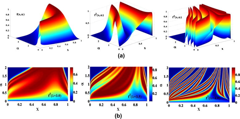
(a) The effect of the function iteration f^m where $f(x\text{,}\alpha \text{,}\lambda )=4x^{\alpha }(l-x^{\alpha })$ for m = {1, 2, 4} and (b) the projection of the fifth iteration for different values of λ = {3.0, 3.5, 4.0}.

Effect of λ with fixed m = 5

As known from the conventional case, the parameter λ affects the map response. Fig. 1b shows the projection of the fifth iterated function f⁵ in the α–x plane for different values of λ. The range of this function increases as λ increases from less than 0.8 when λ = 3.0 up to the full range [0, 1] when λ = 4.0. Moreover, the number of peaks increases as shown from Fig. 1b from the merging of the red color (high values) with the blue (low values), and the contours become more nonlinear as λ increases from 3.0 up to 4.0.

The nontrivial fixed points versus λ

The fixed points can be calculated from $x^{\ast }=f(x^{\ast }\text{,}\lambda \text{,}\alpha )$ then the equation that controls the value of x^* is given by $\lambda {(x^{\ast })}^{2\alpha }-\lambda {(x^{\ast })}^{\alpha }+x^{\ast }=0$. Let us assume α = 0.1 k, where k ∊ N⁺ and y = x^0.1 which transforms the previous equation into a polynomial as $\lambda y^{2k}-\lambda y^k+y^{10}=0$ As long as the parameter λ is known the roots of the previous equation can be easily obtained. Fig. 2 shows the nontrivial solution (x^* ≠ 0) where x^* increases as λ increases when α < 1. In addition, the nonlinearity of the curve x^* also increases. As α becomes very small, the value of x^* becomes closer to zero (trivial solution). The stability criteria of these points is classified based on the derivative at these points for example if $|f^{\prime }(x^{\ast }\text{,}\lambda \text{,}\alpha )|<1$ then this point is a sink point (stable point), however if $|f^{\prime }(x^{\ast }\text{,}\lambda \text{,}\alpha )|>1$ this point will be a source (unstable point). The derivative $f^{\prime }=\frac{\partial f}{\partial x}$ is given by

$$f^{\prime }(x^{\ast }\text{,}\lambda \text{,}\alpha )=\lambda \alpha {(x^{\ast })}^{\alpha -1}(1-2{(x^{\ast })}^{\alpha })$$ (3)

Therefore, the critical point λ_s is the value of λ when the absolute derivative becomes one. This value depends on the relationship between the fixed point x^* and $x_p=\sqrt[\alpha ]{0.5}$ as follows

$${\lambda }_s=\left\{\begin{array}{cc}\frac{1}{\alpha {(x^{\ast })}^{\alpha -1}(1-2{(x^{\ast })}^{\alpha })}\hfill & x^{\ast }<x_p\hfill \\ 4x_p\hfill & x^{\ast }=x_p\hfill \\ \frac{1}{\alpha {(x^{\ast })}^{\alpha -1}(2{(x^{\ast })}^{\alpha }-1)}\hfill & x^{\ast }>x_p\hfill \end{array}\right)$$ (4)

When α = 0.1, the system has a single fixed point in the full range of λ and it is always stable. However, as α increases, the absolute derivative $|f^{\prime }(x^{\ast }\text{,}\lambda \text{,}\alpha )|$ begins to exceed one as λ increases as shown from Fig. 2a. For example when α = 0.5, then $f(x\text{,}\lambda \text{,}\alpha )=\lambda \sqrt{x}(1-\sqrt{x})$, the fixed point x^* is given by $x^{\ast }={(\lambda /(\lambda +1))}^2$ and x_p = 0.25. The derivative at this fixed point is given by $f^{\prime }(x^{\ast }\text{,}\lambda \text{,}0.5)=0.5(1-\lambda )$. Therefore, this fixed point is stable only in the range λ ∊ (0, 3). If λ > λ_s = 3, then this point will be unstable and bifurcation starts. Similarly for other cases when α < 1, the system has a fixed point in the range of λ ∊ (0, λ_max).

Fig. 2.

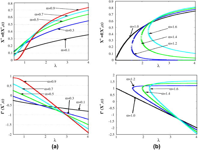
The fixed points and their derivatives versus for different values of (a) α < 1 and (b) α > 1.

When α > 1.0, the curves of x^* become more nonlinear as shown in Fig. 2b. By simple differentiation and analysis, the critical value x_λ at which $\frac{\partial \lambda }{\partial x^{\ast }}=0$ is given by $x_{\lambda }={(\frac{1-\alpha }{1-2\alpha })}^{1/\alpha }$ and the critical value ${\lambda }_c=\frac{x_{\lambda }}{x_{\lambda }^{2\alpha }-x_{\lambda }^{\alpha }}$. These critical values are located in the acceptable range if α > 1.0 as shown from Table 1, and also from Fig. 2b. By using the definition of λ_c and x_λ in the calculation of the derivative at that point where $|f^{\prime }(x_{\lambda }\text{,}{\lambda }_c\text{,}\alpha )|=1$ is the stability limit of the fixed points. Therefore, the nontrivial fixed points in the case when α > 1.0 will be stable in the range λ ∊ (λ_c, λ_s) where λ_s is given by (4).

Table 1.

The values of x_λ and λ_c for different α.

α	1.1	1.2	1.3	1.4	1.5	1.6	1.7	1.8	1.9	2
xλ	0.104	0.198	0.276	0.34	0.397	0.444	0.484	0.5195	0.55	0.5774
λc	1.3674	1.6136	1.81	1.976	2.117	2.238	2.34479	2.43896	2.5228	2.5981

The bifurcation diagrams versus λ for α < 1

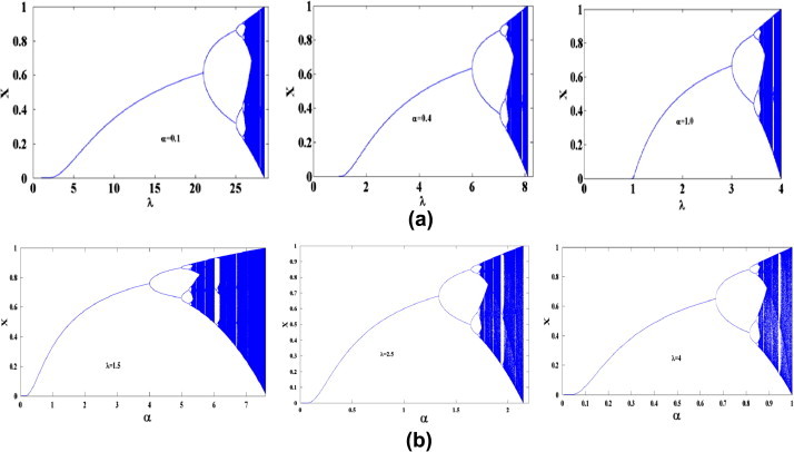
From the previous analysis, the bifurcation diagram of the proposed map depends on some critical values. All bifurcation diagrams are studied in the full range of λ which is (0, 4]. Fig. 3 illustrates the effect of α on the bifurcation diagram versus λ. When α = 0.1, no bifurcation will occur as expected since the system has a fixed point in the full range of λ. As α = 3.0 the stable fixed points exist in the range λ ∊ (0, λ_s) as shown in Fig. 2a, after that range, bifurcation occurs as shown in Fig. 3. Therefore, for fixed value of λ, the behavior of the system will be changed with different α. For example at λ = 3.8, the system response changed from fixed points, period two, multiple periods, and chaos when α equals to 0.1, 0.3, 0.5 and α > 0.7 respectively. As α = 1, the conventional bifurcation diagram is obtained.

Fig. 3.

The bifurcation diagram of the first proposed logistic map versus A for different values of α = {0.1, 0.3, 1.1, 2.5}.

The bifurcation diagrams versus λ for α > 1

As discussed in the fixed points subsection, when α > 1 this logistic map has a fixed point for each λ in the interval λ ∊ (λ_c, λ_s). Therefore, the bifurcation diagram suffers from discontinuities once the parameter α > 1 as shown from Fig. 3 where the fixed points appeared suddenly at λ = λ_c as discussed in Table 1. For example when α = 2.5, the bifurcation diagram starts very close to λ = 2.9 with a single solution (fixed point) until λ ≈ 3.3 where bifurcation begins. It is very clear that the bifurcation diagram has a similar shape to the conventional case. However as α becomes greater than one the range of λ for a stable behavior either fixed, periodic or chaotic shrinks from both sides as shown in Fig. 3 when α = 2.5 where the maximum value of λ for a chaotic solution is less than 3.8. Hence, as α increases more, the domain of λ will decay from both sides.

The bifurcation diagrams versus α for different λ

Since this generalized logistic map has another parameter α it is possible to study the bifurcation diagram with respect to α for fixed values of λ as shown in Fig. 4. For λ = 1, the only acceptable range of α is (0, 1] and in this range the system has only one fixed nontrivial solution. As λ > 1 the response will be different as shown in Fig. 3 where the range of acceptable α for nontrivial solution is related to λ_c. For example when λ = 2 the system has a single nontrivial fixed point up to α = 1.416. Avery interesting curve is found when λ = 3 where the system has period two in the range α ∊ (0.5, 1). Otherwise, the system has a single nontrivial solution in the ranges (0, 0.5] and [0.5, 2.792). In the final curve when λ = 4 we see that chaos exists in a wide range of α and disappears at higher values of α as verified before.

Fig. 4.

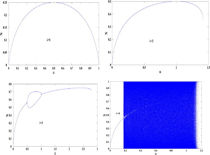
The bifurcation diagram of the first proposed logistic map versus a for different values of X = 1, 2, 3, and 4.

Second generalized logistic map $x_{n+1}=\lambda x_n(1-x_n^{\alpha })$

Let us define $p(x\text{,}\lambda \text{,}\alpha )=\lambda x(1-x^{\alpha })$ where its peak exists at $x=x_p={\left(\frac{1}{\alpha +1}\right)}^{1/\alpha }$ which monotonically increases as α increases. As α → 0 the peak value x_p tends to e⁻¹ however as α → ∞ the value of x_p → 1. The range of λ to guarantee that $p^m(x\text{,}\lambda \text{,}\alpha )$ is always in the range [0, 1] is given by λ ∊ (0, λ_max) where ${\lambda }_{\max }=\frac{{(\alpha +1)}^{\frac{1}{\alpha }+1}}{\alpha }$. As α changes from 0 to ∞, the values of λ_max changes from ∞ to 1.0. So, λ_max is affected by the parameter α in this case since $p(x\text{,}\lambda \text{,}\alpha )$ is different than the previous case $f(x\text{,}\lambda \text{,}\alpha )$ where this range was fixed.

The fixed points

The fixed points can be calculated from $x^{\ast }=p(x^{\ast }\text{,}\lambda \text{,}\alpha )$ which is given by $x^{\ast }={(\frac{\lambda -1}{\lambda })}^{1/\alpha }$ which exists only when λ > 1. The derivative at the fixed point is given by $p^{\prime }(x^{\ast }\text{,}\lambda \text{,}\alpha )=\alpha (1-\lambda )+1$, then for stability the range of λ at which this point becomes stable is given by λ ∊ (1, ${\lambda }_s=\frac{\alpha +2}{\alpha }$). Then for all cases belonging to this generalized map, the bifurcation begins at λ = 1 independent of the parameter α. Therefore the range of bifurcation should be a subset of the range (1, λ_max) and as long as α increases this range will decrease as shown in Fig. 5. For example when α = 0.5, then this generalized logistic map will be $p(x\text{,}\lambda \text{,}0.5)=\lambda x(1-\sqrt{x})$ where $(x_p\text{,}{\lambda }_{\max }\text{,}{x}^{\ast }\text{,}{\lambda }_s)=(\frac{4}{9}\text{,}6.75\text{,}{\left(\frac{\lambda -1}{\lambda }\right)}^2\text{,}5.0)$. So, in this case the system has a fixed point x^* in the range λ ∊ (1, 5) and then period two will begin after λ = 5.0 and the bifurcation increases as λ increases up to its maximum value λ_max.

Fig. 5.

The bifurcation diagram of the second proposed logistic map (a) versus A for different values of α = {0.1, 0.4, 0.7, 1.0, 100} and (b) versus a for different values λ = {1.5, 2.5, 4.0}.

The fifth iteration α ∊ [0, 2] for different λ < λ_max = 2.5981

The effect of λ in the 5th iteration $p^5(x\text{,}\lambda \text{,}\alpha )$ where the function value increases as λ increases is studied. The function value at λ = 0.5 < 1 is very small compared to higher values of λ_max > λ > 0.5 where this value will approach one as λ approaches its maximum value λ_max = 2.5981. In addition, the number of peaks increases as λ increases and at higher values of α.

The bifurcation diagrams versus λ for different α

The bifurcation diagrams with respect to λ for different values of α are shown in Fig. 5. It is clear that the fixed point appears in all cases at λ = 1 however the range of obtaining chaos is widely different with α. When α = 0.1 the first bifurcation happens at λ_s = 21 and chaos happens at λ_max = 28.53 whereas these values shrink to λ_s = 6 and λ_max = 8.117 at α = 0.4 and shrink more up to λ_s = 3 and λ_max = 4 at the conventional case (α = 0.4) as shown in Fig. 5. The range from the first bifurcation to chaos in case α = 1.5, 2.0, 3.0, and 5.0 is given by (2.33, 3.07), (2, 2.598), (1.667, 2.116), and (1.4, 1.717) respectively. For α = 100 this range will shrink to (1.02, 1.0577) where the bifurcation happens at λ = 1.02 and the system behaves chaotically at λ = 1.0577 with an output covering all the range [0, 1].

The bifurcation diagrams versus α for different λ

Similarly the bifurcation diagrams with respect to α are shown in Fig. 5 for different values of λ = 1.5, 2.5, and 4.0. All the bifurcation diagrams are similar to the bifurcation diagram shown before with respect to λ. It is noted that, the dependence of the functions f and p are different with respect to α as shown from the bifurcation diagrams of Figs. 4 and 5 respectively.

Third generalized logistic map $x_{n+1}=\lambda x_n^{\alpha }(1-x_n)$

Let us define $s(x\text{,}\lambda \text{,}\alpha )=\lambda x^{\alpha }(1-x)$ where the peak of this exists at $x=x_p=\frac{\alpha }{\alpha +1}$ which monotonically increases as α increases. As α → 0 the peak value x_p tends to 0 however as α → ∞ the value of x_p → 1. The range of λ to guarantee that $s^m(x\text{,}\lambda \text{,}\alpha )$ is always in the range [0, 1] is given by λ ∊ (0, λ_max) where ${\lambda }_{\max }=\frac{{(\alpha +1)}^{\alpha +1}}{{\alpha }^{\alpha }}$. Then if α increases, λ_max will increase as shown in Fig. 6. Using simple calculations, the fixed point x^* will be stable in the range max(0, $\frac{\alpha -1}{\alpha }$) < x < $\frac{\alpha +1}{\alpha +2}$ which is equivalent to 0 < λ < $\frac{{(\alpha +2)}^{\alpha }}{{(\alpha +1)}^{\alpha -1}}={\lambda }_s$ in case if α < 1 and ${\lambda }_{\min }=\frac{{\alpha }^{\alpha }}{{(\alpha +1)}^{\alpha -1}}<\lambda <\frac{{(\alpha +2)}^{\alpha }}{{(\alpha +1)}^{\alpha -1}}={\lambda }_s$ when α > 1. Therefore, the range of operating λ for fixed α is the distance between λ = 0 and the dashed line (horizontal line λ_max) as clear in the case of α = 0.5 in Fig. 6a. The range of all possible outputs is given from the intersection between the dashed line with the solid line. However, as α > 1 the curve λ_c has a minimum (non-invertible) then for constant α the fixed point will not start from λ = 0 and the starting point (λ_min) increases as α increases. Hence, the maximum range of acceptable λ for nontrivial solution is (λ_min, λ_max). For example when α = 1.5, the system has only one trivial solution in the interval (0, 2.6), the single nontrivial fixed point exists from λ_min ≈ 2.6 and then bifurcation to chaos appears in the interval below λ_max = 5.38 as shown in Fig. 6a and its bifurcation diagram in Fig. 6b. As α increases both the λ_min and λ_max increase where the system has a nontrivial solution as shown in Fig. 6a and b in the case α = 6.3.

Fig. 6.

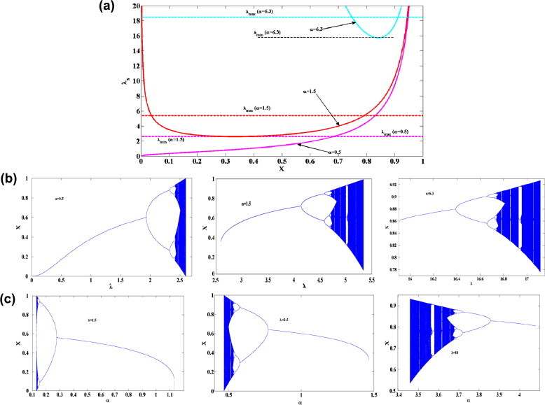
(a) The range of A_s versus x for three different values of a = {0.5, 1.5, 6.3}, (b) the bifurcation diagram versus A for different values of a = {0.1, 0.5, 6.3}, and (c) the bifurcation diagram versus a for different values of A = {1.5, 2.5, 10}.

The bifurcation diagram of the third proposed logistic map versus the arbitrary power is shown in Fig. 6c where the chaotic response happens at the lower values of α. As α increases the system behavior transforms from chaotic response, to periodic until it reaches fixed point. In addition, as λ increases both the lower and upper values of α for nontrivial solutions are increased.

Comparison and calculation of Lyapunov exponent

From the previous sections, we found that the proposed logistic maps have different characteristics and cover all possible cases. For example, the bifurcation range is:

• •λ ∊ (0, 4) with fixed limits as in the first proposed map when α < 1,
• •λ ∊ (λ_c, 4) with variable start limit as in the first proposed map when α > 1,
• •λ ∊ (0, λ_max) with variable end limit as in the third proposed map when α < 1,
• •λ ∊ (1, λ_max) with variable end limit as in the second proposed map,
• •λ ∊ (λ_min, λ_max) with variable start and end limits as in the third proposed map when α > 1.

Moreover, the bifurcation diagram with respect to the new parameter α for the second and third proposed maps has similar properties as the conventional logistic map which increases the design flexibility. The time domain output and the illustration of Cobweb method for the three proposed maps are shown in Table 2 when the new parameter α = 0.5 and in the chaotic range of λ.

Table 2.

Comparison between the main aspects of the proposed generalized logistic maps.

Map	$x_{n+1}=\lambda x^{\alpha }(1-x^{\alpha })$	$x=x_{n+1}=\lambda x(1-x^{\alpha })$	$x_{n+1}=\lambda x^{\alpha }(1-x)$
Critical values	$x=x_p={}^{\alpha }\sqrt{0.5}\text{,}{\lambda }_{\max }=4$	$x=x_p={\left(\frac{1}{\alpha +1}\right)}^{1/\alpha }\text{,}{\lambda }_{\max }=\frac{{(\alpha +1)}^{\frac{1}{\alpha }+1}}{\alpha }$	$x=x_p=\frac{\alpha }{\alpha +1}\text{,}{\lambda }_s=\frac{{(\alpha +2)}^{\alpha }}{{(\alpha +1)}^{\alpha -1}}$
	${\lambda }_s=\frac{1}{\alpha {(x^{\ast })}^{\alpha -1}(1-2{(x^{\ast })}^{\alpha })}$	$x^{\ast }={\left(\frac{\lambda -1}{\lambda }\right)}^{\frac{1}{\alpha }}\text{,}{\lambda }_s=\frac{\alpha +2}{\alpha }$	${\lambda }_{\max }=\frac{{(\alpha +1)}^{\alpha +1}}{{\alpha }^{\alpha }}\text{,}{\lambda }_{\min }=\frac{{\alpha }^{\alpha }}{{(\alpha -1)}^{\alpha -1}}$
Range (α < 1)	$\lambda \in (0\text{,}4)$	$(1\text{,}{\lambda }_{\max })$	(0,λmax)
Range (α > 1)	$\lambda \in ({\lambda }_c\text{,}4)$	$(1\text{,}{\lambda }_{\max })$	$({\lambda }_{\min }\text{,}{\lambda }_{\max })$
Bifurcation versus α (α < 1)	• Fixed range of λ	• Fixed starting at λ = 1 but variable end	• Fixed starting point λ = 0 and variable end
	• Bifurcation diagram may not exist for small α	• The system always has bifurcation diagram for all α	• The system always has bifurcation diagram for all a
Bifurcation diagrams versus α (α > 1)	• Bifurcation begins at λ = λc and increases with α	• Fixed start and variable end	• Both ends variables and increases as α increases
	• Bifurcation ends at λ < 4	• The bifurcation range decays as α increase with full bifurcation diagram	• Bifurcation diagram exist in all cases
	• The range of bifurcation decays as α increases
The bifurcation diagrams versus α	• At $\lambda ={\lambda }_{\max }=4$ the output is almost fixed or chaos in a wide range of α	• Exist when λ > 1 with similar to the logistic map Which cover fixed point, bifurcation, up to chaos	Exist when λ > 1 and looks like a mirrored logistic map. Start from chaos to fixed point as α increases
	• The range of α start from 0 and its end varies with λ	• The range of α start from 0 and its end varies with λ	Both ends are variables with λ
Method of cobwebbing for chaotic dynamical behavior at α = 0.5
Lyapunov exponent for different α

The calculation of Lyapunov exponent

To prove the chaotic behavior of the output response, it is required to calculate the Lyapunov exponent which is the major key for chaotic systems. As known from the nonlinear analysis of chaos, it is necessary to have a positive value of the Lyapunov exponent to prove chaotic behavior. Recently [24–28], there are many numerical techniques to calculate the value of the Lyapunov exponent. For the 1-D map defined by x_k+1 = f(x_k, λ), the Lyapunov exponent for the orbit starting at x_o can be calculated by

$$L.E.={\displaystyle \underset{n\to \infty }{\lim }}\left\{\frac{1}{n}{\displaystyle \sum _{i=0}^{n-1}}\ln |f^{\prime }(x_i)|\right\}$$ (5)

where $f^{\prime }(x)$ is the derivative of the function f(x). The Lyapunov exponents of the proposed maps are shown in Table 2. As known the conventional logistic map at λ = 3.9 has a Lyapunov exponent of order 0.496. The effect of the new parameter α in the first proposed map (fixed range) on the Lyapunov exponent is shown in Table 2 where the LE increases as the value of α increases for the same value of λ. Five different cases of the LE for each of the second and third proposed maps are shown in Table 2.

Conclusion

This paper introduces three independent generalized logistic maps of arbitrary order. The summary of the main factors for each proposed map, the critical points, ranges, and some comments on the bifurcation diagrams with respect to the system parameter and also to the arbitrary power are introduced. Moreover, the iterated outputs of the three systems are also introduced where chaotic behavior is verified through the time domain and also by the calculation of the Lyapunov exponent where positive values are obtained. Therefore, the proposed three generalized logistic maps enrich the nonlinear dynamical system through the extra degree of freedom which can be used for the accurate study and modeling of many applications in various fields as in bioengineering and communication security.

References

- 1.Gulick D. McGraw-Hill; New York: 1992. Encounters with chaos. [Google Scholar]
- 2.Ausloos M., Dirickx M. Springer; Berlin/Heidelberg: 2006. The logistic map and the route to chaos from the beginnings to modern applications. [Google Scholar]
- 3.Li T.Y., Yorke J. Period three implies chaos. Am Math Month. 1975;82:985–992. [Google Scholar]
- 4.Pellicer-Lostao C., López-Ruiz R. A chaotic gas-like model for trading markets. J Comput Sci. 2010;1:24–32. [Google Scholar]
- 5.Pearl R. Oxford Medical Publications; 2000. An introduction to medical statistics. [Google Scholar]
- 6.Kinnunen T, Pastijn H. The chaotic behavior of growth processes. ICOTA proceedings, Singapore; 1987.
- 7.Malek K., Gobal F. Application of chaotic logistic map for the interpretation of anion-insertion in poly-ortho-aminophenol films. Synthetic Met. 2000;113:167–171. [Google Scholar]
- 8.Pareek N.K., Patidar V., Sud K.K. Image encryption using chaotic logistic map. Image Vis Comput. 2006;24:926–934. [Google Scholar]
- 9.Andrecut M. Logistic map as a random number generator. Int J Modern Phys B. 1998;12:921–930. [Google Scholar]
- 10.Patidar V., Sud K.K., Pareek N.K. A pseudo random bit generator based on chaotic logistic map and its statistical testing. Informatica. 2009;33:441–452. [Google Scholar]
- 11.Singh N., Sinha A. Chaos-based secure communication system using logistic map. Opt Lasers Eng. 2010;48:398–404. [Google Scholar]
- 12.Barakat ML, Radwan AG, Salama KN. Hardware realization of chaos based block cipher for image encryption. The 23rd international conference on microelectronics (ICM), Tunis; 2011.
- 13.Sarker J.H., Mouftah H.T. Secured operating regions of Slotted ALOHA in the presence of interfering signals from other networks and DoS attacking signals. J Adv Res. 2011;2:207–218. [Google Scholar]
- 14.Lopez-Ruiz R., Fournier-Prunaret D. Complex behaviour in a discrete logistic model for the symbiotic interaction of two species. Math Biosci Eng. 2004;1:307–324. doi: 10.3934/mbe.2004.1.307. [DOI] [PubMed] [Google Scholar]
- 15.Ausloos M., Clippe P., Miskiewicz J., Pekalski A. A reactive lattice-gas approach to economic cycles. Phys A. 2004;344:1–7. [Google Scholar]
- 16.Ausloos M., Miskiewicz J. Delayed information flow effect in economy systems: an ACP model study. Phys A. 2007;382:179–186. [Google Scholar]
- 17.Ausloos M, Miskiewicz J. Influence of information flow in the formation of economic cycle. In: The logistic Map and the Rout to Chaos. Berlin: Springer-Verlag; 2006. p. 223–38.
- 18.Leydesdorff L., Dubois D.M. Anticipation in social systems: the incursion and communication of meaning. Int J Comput Anticipatory Syst. 2004;15:203–216. [Google Scholar]
- 19.Dubois D.M. Introduction to computing anticipatory systems. Int J Comput Anticipatory Syst. 1998;(2):3–14. [Google Scholar]
- 20.Suneel M. Electronic circuit realization of the logistic map. Sadhana. 2006;31(1):69–78. [Google Scholar]
- 21.Radwan A.G., Soliman A.M., EL-sedeek A.L. An inductorless CMOS realization of Chua’s circuit. Chaos Solitons Fractals. 2003;(18):149–158. [Google Scholar]
- 22.Radwan A.G., Soliman A.M., EL-sedeek A.L. MOS realization of the double-scroll-like chaotic equation. IEEE Circ Syst-I. 2003;50(2):285–288. [Google Scholar]
- 23.Sturm R. Modeling the deposition of bioaerosols with variable size and shape in the human respiratory tract – a review. J Adv Res, in press.
- 24.Strogatz S.H. Addison-Wesley; New York: 1994. Nonlinear dynamics and chaos: with applications to physics, biology, chemistry, and engineering. [Google Scholar]
- 25.Nayfeh A.H., Balachandran B. John Wiley & Sons; New York: 1995. Applied nonlinear dynamics: analytical, computational, and experimental methods. [Google Scholar]
- 26.Wolf A., Swift J.B., Swinney H.L., Vastano J.A. Determining Lyapunov exponents from a time series. Phys D: Nonlinear Phenom. 1985;16(3):285–317. [Google Scholar]
- 27.Abarbanel H.D.I. Springer-Verlag; New York: 1996. Analysis of observed chaotic data. [Google Scholar]
- 28.Rosenstein M.T., Collins J.J., DeLuca C.J. A practical method for calculating largest Lyapunov exponents from small data sets. Phys D: Nonlinear Phenom. 1993;65:117–134. [Google Scholar]