

Abstract
We conduct a cross-sectional ecological analysis to examine environmental correlates of active commuting in 39,660 urban tracts using data from the 2010 Census, 2007-2011 American Community Survey, and other sources. The five-year average (2007-2011) prevalence is 3.05% for walking, 0.63% for biking, and 7.28% for public transportation to work, with higher prevalence for all modes in lower-income tracts. Environmental factors account for more variances in public transportation to work but economic and demographic factors account for more variances in walking and biking to work. Population density, median housing age, street connectivity, tree canopy, distance to parks, air quality, and county sprawl index are associated with active commuting, but the association can vary in size and direction for different transportation mode and for higher-income and lower-income tracts.
Introduction
Being physically active is one of the most important steps that people of all ages can take to improve their health (U.S. Department of Health and Human Services, 2008). Current physical activity (PA) guidelines in the U.S. recommend that adults should engage in 150 minutes of moderate-to-vigorous aerobic activity every week, which can include various activity domains such as leisure-time, occupational, household, and transportation (U.S. Department of Health and Human Services, 2008). Active commuting (AC), defined as walking, biking, or taking public transportation to work or school, is an important form of PA in the transportation domain that offers a viable method to achieve PA recommendations by incorporating the needed activity into normal daily life (Shephard, 2008, Bopp et al., 2012, Bopp et al., 2013, Berrigan et al., 2006). Indeed, Healthy People 2020 has identified AC as an important strategy for increasing population-level PA (U.S. Department of Health and Human Services, 2012).
There are many well-documented health benefits of AC, including a reduced risk of all-cause mortality (Andersen et al., 2000), obesity (Lindström, 2008), and cardiovascular disease and risk factors (Hamer and Chida, 2008). In addition, AC can indirectly benefit health by reducing carbon dioxide emissions through less use of vehicles and less traffic congestion (Giles-Corti et al., 2010, Shephard, 2008). There are also economic benefits to individuals through reduced vehicle operating and maintenance costs (Shephard, 2008, Litman and Doherty, 2009). However, despite the multiple benefits, the rate of AC in the U.S. remains low, both in terms of historical trend and when compared with other countries (Bassett Jr, 2012, Kruger et al., 2008).
One of the important factors affecting individuals' AC decisions is the environment (i.e., physical environment) individuals live in, because walking and biking put individuals in closer contact with their environment for a longer period of time when compared with private vehicle travel. For example, pleasant neighborhood environment with tree-lined streets and pedestrian traffic may encourage AC by making walking and biking to work enjoyable, while a high crime rate in the neighborhood may deter individuals from walking and biking to work due to safety concerns. Indeed, among the potential correlates or determinants of PA in general, environmental factors have received much attention in recent years (Bassett Jr, 2012, Bauman et al., 2012). From a public health perspective, an understanding of environmental correlates and determinants of PA is useful because environmental changes may be achieved through public policy with population-wide benefits. However, while consensus has begun to emerge on some environmental factors influencing total PA, few consistent correlates of AC have been identified (Bauman et al., 2012). Understanding correlates of specific domains of PA such as AC is important because evolving research has shown that the etiology of PA is complex and varies by domain, and different attributes of the environment are associated with activities being undertaken for different purposes and in different forms (Bauman et al., 2012, Adams et al., 2013, Sallis et al., 2006).
Evidence from the limited amount of research on environmental correlates of adults' AC is equivocal (Panter et al., 2011, Panter and Jones, 2010). Some studies have related AC to various neighborhood walkability features that include the 3Ds: population density, pedestrian-friendly design, and a diversity of destinations (Cervero and Kockelman, 1997, Berrigan et al., 2010, Badland et al., 2008) while others reported few or no environmental characteristics to be consistently associated with AC, especially when individual and interpersonal characteristics are controlled for (Lemieux and Godin, 2009, Bopp et al., 2013). Overall, research on environmental correlates of AC has been challenged by the limited availability of AC and objectively measured environment data, especially data at the national level.
In this study we aim to analyze environmental correlates of AC in urban U.S. by combining multiple national datasets at the census tract level to investigate three modes of AC: walking to work, biking to work, and taking public transportation to work. In addition, we aim to investigate if the association between environment and AC participation is moderated by neighborhood income status. The income sub-analysis is motivated by the public heath challenge concerning income-related health disparities. It is well established in the literature that lower-income individuals have poorer health outcomes compared to higher-income individuals (Bleich et al., 2012, Cerin et al., 2009). Our preliminary analysis of data has shown significant differences in the relationship between AC prevalence and environmental factors by neighborhood median income, race/ethnic composition, and percent of college-educated population. These three factors are highly correlated as lower median income, higher proportions of minorities, and lower levels of education tend to go together. In this paper we choose to focus on income-based differences while leaving investigations of other differences to future studies, in part because we believe economically-disadvantaged neighborhoods deserve help from public health policy efforts regardless of their racial/ethnic or educational composition.
In taking such an ecological approach, we do not attempt to draw inferences regarding individual level associations. Rather, we seek to add our understanding of environmental correlates of AC from a different angle that can complement existing AC research. While such an ecological analysis cannot identify factors affecting the individual decision-making process and behavior of AC, it is valuable in identifying factors that are associated with aggregate AC participation rates, which is a public health objective in itself regardless of which individuals in the aggregate are participating in AC. In fact, given that recent studies on PA in general and AC in particular have called for policy interventions to modify our environment in order to increase population PA levels (Bassett Jr, 2012, Bauman et al., 2012), a direct assessment of aggregate relationships between environment and AC is critically needed.
Conceptual Framework
We utilize the microeconomic framework of consumer decision-making to guide our analysis by classifying correlates of AC into to two general categories: preferences and constraints (Varian, 1992). Preferences are represented by demographic factors such as age, race/ethnicity, nativity, and education level (Lemieux and Godin, 2009, Bopp et al., 2012, Bauman et al., 2012). The traditional microeconomic consumer decision-making framework focuses only on the income constraint, which includes both income/wealth and relative costs associated with alternative forms of transportation to work. For this study, we extend the traditional framework by adding three categories of non-monetary constraints that can affect AC decisions: environment, neighborhood safety, and commuting distance. These non-monetary constraints are important because, for example, a walkable and safe neighborhood that is close to work destinations is likely to encourage AC due to lower costs associated with walking/biking, whereas a neighborhood with poor walkability and/or a high crime rate is likely to discourage AC by increasing the total costs associated with walking/biking. Figure 1 illustrates our conceptual framework.
Figure 1. Conceptual framework of determinants/corrletes of active commuting.
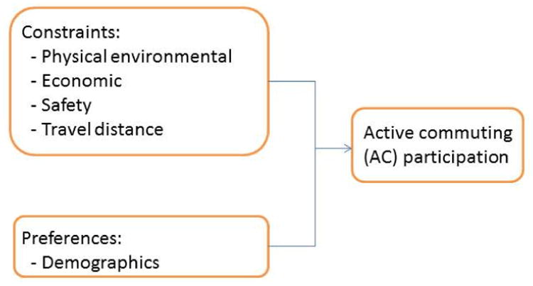
Past studies have described neighborhood walkability by neighborhood 3D's of density, design, and diversity (Cervero and Kockelman, 1997). Neighborhoods with higher population density, more pedestrian-friendly design features such as better street connectivity, and better land-use diversity are considered more walkable. However, empirical findings regarding the relationship between specific measures of neighborhood features and AC are limited. Therefore, instead of forming specific directional hypotheses for individual variables, we form a general hypothesis that environmental factors that can reduce the total cost of AC would be positively associated with AC participation, while environmental factors that may increase the total cost of AC would be negatively associated with AC participation. In addition, because the cost-benefit calculation is likely moderated by income constraints, we expect the relationship between environment and AC to be different between higher-income and lower-income neighborhoods.
Among the five groups of AC correlates (i.e., environment, neighborhood safety, commuting distance, economic, and demographics), our focus is on the environment and its interaction with economic constraints. Other factors are controlled in our analysis. In the context of an ecological study, these variables may capture both the aggregate of individual characteristics and their interactions at the interpersonal and neighborhood levels, as interpersonal factors such as social support (Bauman et al., 2012, Bopp et al., 2013, Bopp et al., 2012) have also been found to affect AC decisions.
Data and Variables
Our primary data sets are the 2010 Decennial Census (U.S. Bureau of the Census, 2010) and the 2007-2011 American Community Survey (U.S. Bureau of the Census, 2014a). A challenging question in studying environment correlates of health outcome and health behavior concerns how to define the relevant geographic scale, which is an example of the well-known Modifiable Areal Unit Problem (MAUP) associated with the use of geographically aggregated data (Openshaw, 1977). Conceptually, the relevant geographic scale is likely to differ across individuals, places, environmental factors, and outcomes being studied. Empirically, when one geographic scale has to be chosen, among various scales used ranging from census block group to states, census tract-level analyses have been found to most consistently indicate associations between neighborhood characteristics and resident's health (Fan et al., 2014a, Krieger et al., 2003). Therefore, we choose to use census tract as the main geographic unit in this study. Census tracts are small (between 1,200 and 8,000 residents), relatively permanent statistical subdivisions of a county. They are as homogenous as possible by design with respect to population characteristics, economic status, and living conditions when first established (U.S. Bureau of the Census, 2014b). In addition, in the context of AC, recognizing that many commuters may travel across more than one tract, especially if biking or public transportation are used, we incorporate several additional measures at the county level.
This study only focuses on urban areas because rural areas have drastically different physical features that are likely to render very different environment-AC relationships. The rural-urban commuting area (RUCA) codes, developed by the U.S. Department of Agriculture, are used to define urban tracts (U.S. Department of Agriculture, 2013). The RUCA codes adopt the metropolitan and micropolitan terminology used by the Office of Management and Budget but provide a more detailed geographic pattern of urban and rural areas by using census tracts instead of counties as building blocks. For this study we define urban as all census tracts with RUCA codes between 1 and 3, which includes tracts located in metropolitan urban areas (i.e., areas with a population of at least 50,000).
AC measures
Three tract-level aggregate AC measures are five-year averages generated from the 2007-2011 American Community Survey: (1) percent of workers 16+ who walk to work, (2) percent of workers 16+ who bike to work, and (3) percent of workers 16+ who utilize public transportation to work. We use all three variables in order to capture the multiple dimensions of AC.
Environment
Tract population density (1,000 per square mile) comes from the 2010 U.S. Census and measures the density aspect of the 3D's. Tract median housing age is computed from tract median housing build year from the 2007-2011 American Community Survey and is used as a proxy measure of neighborhood walkability because older neighborhoods were built before people began to rely on cars and are typically more walkable than newer neighborhoods with better land use diversity, narrower streets, and more extensive sidewalks (Boer et al., 2007, Smith et al., 2008, Berrigan and Troiano, 2002). The design aspect of the 3D's is captured by a tract-level street connectivity measure, defined as the number of intersections per square kilometer in the tract. This measure is constructed from spatial data including census tracts and road networks from the data CD-ROMs distributed with ArcGIS 9.3 by the Environmental System Research Institute (ESRI) and the StreetMap USA file (a TIGER 2000-based streets data set enhanced by ESRI and Tele Atlas) using the ArcGIS network analysis module (Environmental Systems Research Institute, 2010). Only roads with the speed limit of 25 miles per hour or lower are extracted as roads with higher speed limits are considered highways or major roads and do not contribute to street connectivity (Wang et al., 2013). A greenness measure is derived from the tree canopy dataset in the National Land Cover Database 2001 that provides tree canopy density at a spatial resolution of 30 meters (Homer et al., 2007). Using this dataset, a tract-level aggregate tree canopy density measure is generated to represent the average of the percentages of tree canopy coverage associated with pixels that fell in each tract. A tract-level park access variable is constructed from the 2006 park GIS layer in the ESRI ArcGIS 9.3 Data DVD (Environmental Systems Research Institute, 2010). Seven parks (Miller, 1956) closest to all census block centroid are identified, and average distances from the census block centroid to each of these parks weighted on population and park sizes are calculated. These distances are then aggregated to the census tract level (Zhang et al., 2011). For air quality, we use data from the Environmental Protection Agency (EPA) to create a dummy variable indicating EPA air quality nonattainment status at the county level (U.S. Environmental Protection Agency, 2006). In addition, because many commuters may travel across more than one tract, especially if biking or public transportation are used, we include the 2010 county-level sprawl index, developed by Ewing and his colleagues (Ewing et al., 2014), to provide a summary measure of the physical environment at the county level. The sprawl index captures four dimensions of development density, land use mix, population and employment centering, and street accessibility. It has a mean of 100 and a standard deviation of 25, with higher scores indicating more compactness and lower scores indicating more urban sprawl (Ewing et al., 2014).
Economic measures
Economic variables include tract-level median household income (in $1,000), median housing value (in $10,000), and percent of housing units that are owner-occupied. In addition to the directly available variables in the 2010 Census, we also create a measure of tract-level income inequality, the Gini coefficient (Kennedy et al., 1996), using the aggregate income data from the 2007-2011 American Community Survey and applying a program developed in STATA (Whitehouse, 1995).
Safety
Because tract-level crime data are unavailable, number of crime per 1,000 persons at the county level are obtained from the 1999-2008 Uniform Crime Reporting Program data from the National Archive of Criminal Justice Data, which contain details arrest data for both Part I (e.g., murder, rape, robbery) and Part II (e.g., vandalism, weapons violations, sex offenses, drug and alcohol abuse violations) offences.
Commuting distance
Commuting distance is captured by tract percent of workers 16+ who have long commute of more than one hour.
Demographics
Demographic variables include tract percent of people who live in college dorms, percent of people who live in military quarters, residents median age, percent of Asian Americans, percent of non-Hispanic blacks, percent of Hispanics, percent of foreign-born population, and percent of residents 25+ with a college degree or higher. These variables, obtained or constructed from the 2010 Census, are typically used as preference indicators because people with different age, gender, culture, and education tend to have different taste and preferences in their decision-making.
Total number of tracts included in this study is 39,660. Among these tracts, 11,158 tracts have more than 20% of individuals below poverty threshold and are thus defined as lower-income (LI) tracts, in line with the Census definition of “poor areas” (U.S. Bureau of the Census, 2011). The remaining 28,502 tracts are classified as higher-income (HI) tracts.
Analytical Method
Because we have two levels of geographical aggregation: tract and county, multilevel models are used for our regression analyses. The main purpose of using multilevel model in this case is to account for the clustering of tracts within counties. Regression analyses are conducted separately on three dependent variables: tract-level percent walking to work, percent biking to walk, and percent taking public transportation to work, first using all tracts, then separately for LI tracts and HI tracts. In addition, we estimate full interaction models for all tracts by adding interaction terms of the LI/HI tract dummy variable with all independent variables in order to test the statistical significance of the coefficient for each independent variable between HI and LI tracts. We also explore nonlinear specifications of the models, including both quadratic and log specifications for all continuous environmental and income variables and some demographic variables to investigate potential nonlinear relationships.
In addition, for general model diagnostics such as multicollinearity tests and model fitness, we also conduct single level OLS regression analyses adjusting for clustering of tracts within counties. The multilevel models are estimated using Proc Glimmix and single level models are estimated using Proc Surveyreg in SAS 9.2 (http://www.sas.com/).
Results
Table 1 provides descriptive statistics of the variables, for all urban tracts included in this study and by tract income status. The five-year average (2007 to 2011) for AC prevalence is 3.05% for walking, 0.63% for biking, and 7.28% for taking public transportation to work. Participation rates are significantly higher for LI tracts than for HI tracts for all three modes. For walking to work, the rate is 5.07% for LI tracts compared with 2.26% for HI tracts. For biking to work, the rate is 0.94% for LI tracts compared with 0.51% for HI tracts. For public transportation to work, the rate is 11.30% for LI tracts compared with 5.71% for HI tracts.
Table 1. Descriptive Statistics: All tracts and by income status.
| All tracts (n=39,660) | Higher-income tracts (n=28,502) | Lower-income tracts (n=11,158) | ||||
|---|---|---|---|---|---|---|
| Variables | Mean | Std | Mean | Std | Mean | Std |
| Active commuting variables: | ||||||
| Tract % workers 16+ walking to work | 3.05 | 5.30 | 2.26 | 3.98 | 5.07 | 7.33 |
| Tract % workers 16+ biking to work | 0.63 | 1.63 | 0.51 | 1.30 | 0.94 | 2.22 |
| Tract % workers 16+ taking public transportation to work | 7.28 | 13.37 | 5.71 | 11.73 | 11.30 | 16.17 |
| Environment: | ||||||
| Tract pop. density (1,000/sq mile) | 6.81 | 12.86 | 5.49 | 10.84 | 10.16 | 16.50 |
| Median housing age | 43.52 | 16.82 | 40.69 | 16.26 | 50.74 | 16.03 |
| Tract intersection density/sq kilometer | 103.17 | 76.18 | 93.24 | 69.92 | 128.51 | 85.13 |
| Tract % area green canopy | 17.44 | 17.72 | 19.75 | 18.52 | 11.54 | 13.81 |
| Average distance to 7 closest parks | 4.02 | 6.55 | 3.97 | 6.23 | 4.14 | 7.30 |
| EPA poor air quality status | 0.69 | 0.46 | 0.69 | 0.46 | 0.67 | 0.47 |
| County urban sprawl index | 128.36 | 39.44 | 126.46 | 38.02 | 133.22 | 42.47 |
| Economic factors: | ||||||
| Tract med. income (in $1,000) | 58.24 | 29.23 | 68.46 | 27.83 | 32.12 | 10.48 |
| Tract Gini coefficient (%) | 39.02 | 4.87 | 37.90 | 4.40 | 41.90 | 4.83 |
| Tract med. housing value (in $10,000) | 25.75 | 19.56 | 29.22 | 20.17 | 16.89 | 14.55 |
| Tract % housing owner-occupied | 0.62 | 0.23 | 0.70 | 0.19 | 0.42 | 0.19 |
| Safety: | ||||||
| County total crime/1,000 people | 40.73 | 20.21 | 38.48 | 19.12 | 46.76 | 21.76 |
| Commuting distance | ||||||
| Tract % 16+ commuting 1 hour+ | 8.16 | 7.73 | 8.16 | 7.59 | 8.15 | 8.09 |
| Demographics: | ||||||
| Tract % living in college dorms | 0.64 | 4.91 | 0.35 | 3.18 | 1.36 | 7.68 |
| Tract % living in military quarters | 0.04 | 1.36 | 0.05 | 1.56 | 0.01 | 0.58 |
| Tract median age | 37.69 | 6.79 | 39.73 | 6.04 | 32.49 | 5.74 |
| Tract % Asians | 5.00 | 8.84 | 5.56 | 9.23 | 3.58 | 7.59 |
| Tract % Blacks | 16.20 | 24.86 | 9.73 | 17.30 | 32.72 | 32.43 |
| Tact % Hispanics | 16.87 | 21.71 | 12.92 | 16.59 | 26.95 | 28.82 |
| Tract % foreign-born | 13.97 | 14.31 | 12.89 | 13.25 | 16.72 | 16.39 |
| Tract % 25+ college educated | 28.76 | 19.13 | 33.68 | 18.61 | 16.20 | 14.00 |
Note: All differences between higher-income tracts and lower-income tracts are statistically significant at 99% confidence level, with the exception of percent with long commuting distance.
Significant differences exist for almost all variables between LI and HI tracts, with the exception of percent with long commuting distance. For environment, compared with HI tracts, LI tracts have higher population density, older housing stock, and a higher level of street connectivity. The county sprawl index indicates that LI tracts are more likely to locate in compact counties than HI tracts. These differences suggest that LI tracts are generally more walkable than HI tracts. In addition, compared with HI tracts, LI tracts have smaller green canopy coverage and longer average distance to parks, but are located in counties slightly less likely to have poor air quality.
Considering economic and safety variables, LI tracts have lower median household income, lower medium housing value, higher tract-level income inequality, and a lower percent of owner-occupied housing units. LI tracts also have higher county-level crime rate than HI tracts. For demographics, LI tracts have higher percentages of blacks, Hispanics, foreign-born, and residents living in college dorms, but lower percentages of Asians, residents living in military quarters, and college-educated. Tract median age is lower for LI tracts than HI tracts.
For multivariate models, single-level regression models are first estimated for diagnostic purpose and to obtain approximate model fitness information. In Table 2 we present approximate R2 statistics for each subgroup of variables separately in order to capture the relative contribution of each group of variables. Note that the R2's for the subgroups do not add up to the total model R2 because the subgroups of variables typically have some correlations with each other. For example, tracts with a higher percent of residents living in college dorms (a demographic variable) is likely to also have a lower percent of people with long commute (a commuting distance variable). However, the correlations are not high enough to cause problems as collinearity diagnostics reveal no problematic multicollinearity issues. Our exploration into nonlinear specification of the models show that for walking to work, a quadratic specification for all continuous environmental variables has a better fit with a lower AIC value. However, for biking to work and public transportation to work, the model fit is better for the linear specification. In the interest of cross-model consistency and model simplicity, we choose to report results from the linear models while additional results are available from authors upon request.
Table 2. Model R2's and R2's for subgroups of variables.
| % Walking to work | % Biking to work | % Public transportation to work | |||||||
|---|---|---|---|---|---|---|---|---|---|
| All tracts | Higher income tracts | Lower income tracts | All tracts | Higher income tracts | Lower income tracts | All tracts | Higher income tracts | Lower income tracts | |
| All variables | 0.48 | 0.46 | 0.50 | 0.19 | 0.19 | 0.21 | 0.78 | 0.78 | 0.80 |
| Environment | 0.18 | 0.23 | 0.11 | 0.05 | 0.08 | 0.02 | 0.67 | 0.67 | 0.69 |
| Economic | 0.24 | 0.20 | 0.24 | 0.09 | 0.09 | 0.06 | 0.33 | 0.29 | 0.37 |
| Safety | 0.00 | 0.00 | 0.00 | 0.00 | 0.01 | 0.00 | 0.00 | 0.00 | 0.01 |
| Commuting distance | 0.00 | 0.00 | 0.00 | 0.01 | 0.00 | 0.01 | 0.33 | 0.29 | 0.46 |
| Demographics | 0.28 | 0.25 | 0.34 | 0.08 | 0.07 | 0.16 | 0.31 | 0.34 | 0.26 |
Note: R2's for subgroups of variables do not add up to total R2's for model including all variables due to some correlation between subgroups of variables.
For all-tract models, among the three AC modes, the model for public transportation has the highest R2 at 0.78, followed by the model for walking to work at 0.48, with biking to work having the lowest R2 at 0.19. The overall model R2's are similar for HI and LI tracts for all three modes. However, relative contribution of subgroups of variables differs. For both the walking and biking models, the environmental variables account for much less variance for LI tracts (R2 =0.11 for walking and R2 =0.02 for biking) than HI tracts (R2 = 0.23 for walking and R2 = 0.08 for biking). In contract, demographic variables account for a much larger proportion of variances in LI tracts (R2 = 0.34 for walking and R2 = 0.16 for biking) than HI tracts (R2 = 0.25 for walking and R2 = 0.07 for biking). For public transportation to work, there is virtually no difference between HI and LI tracts in how much variance the environmental variables explain. However, income and commuting distance variables account for more variances in LI tracts (R2 =0.37 and 0.46, respectively) compared with HI tracts (R2 = 0.29 for both). In contract, demographic variables explain more variance in HI tracts (R2 = 0.34) compared with LI tracts (R2 = 0.26).
Table 3 presents the estimated regression coefficients for the all-tract models, together with their statistical significance. Below we summarize the key results.
Table 3. Regression results for three active commuting modes for all-tract models.
| % Walking to work | % Biking to work | % Public transportation to work | ||||
|---|---|---|---|---|---|---|
| Variables | Coefficient | Coefficient | Coefficient | |||
| Intercept | 4.885 | *** | 1.675 | *** | -7.345 | *** |
| Environment: | ||||||
| Tract pop. density (1,000/sq mile) | 0.033 | *** | -0.001 | 0.244 | *** | |
| Median housing age | 0.013 | *** | 0.017 | *** | 0.037 | *** |
| Tract intersection density/sq kilometer | 0.006 | *** | 0.001 | *** | 0.000 | |
| Tract % area green canopy | -0.012 | *** | -0.001 | ** | 0.004 | |
| Average distance to 7 closest parks | 0.036 | *** | 0.005 | ** | 0.019 | ** |
| County EPA poor air quality status | 0.112 | -0.103 | * | -0.100 | ||
| County urban sprawl index | 0.010 | *** | -0.001 | 0.090 | *** | |
| Economic: | ||||||
| Tract med. income (in $1,000) | -0.019 | *** | -0.015 | *** | -0.002 | |
| Tract Gini coefficient (%) | 0.041 | *** | -0.004 | ** | -0.021 | *** |
| Tract med. housing value (in $10,000) | 0.033 | *** | 0.011 | *** | 0.021 | *** |
| Tract % housing owner-occupied | -6.681 | *** | -0.700 | *** | -9.167 | *** |
| Safety: | ||||||
| County total crime/1,000 people | -0.013 | *** | 0.002 | ** | -0.053 | *** |
| Community distance: | ||||||
| Tract % 16+ commuting 1 hour+ | -0.028 | *** | -0.002 | 0.291 | *** | |
| Demographics: | ||||||
| Tract % living in college dorms | 0.403 | *** | -0.001 | -0.027 | *** | |
| Tract % living in military quarters | 0.398 | *** | -0.020 | *** | -0.038 | ** |
| Tract median age | -0.025 | *** | -0.028 | *** | 0.055 | *** |
| Tract % Asians | 0.014 | *** | -0.008 | *** | 0.037 | *** |
| Tract % Blacks | -0.024 | *** | -0.005 | *** | 0.091 | *** |
| Tact % Hispanics | -0.014 | *** | 0.000 | 0.056 | *** | |
| Tract % foreign-born | -0.009 | *** | -0.004 | *** | -0.035 | *** |
| Tract % 25+ college educated | 0.025 | *** | 0.029 | *** | 0.050 | *** |
p-value <0.01,
p-value <0.05,
p-value<0.1
Environment
On average, an increase of tract population density is associated with higher prevalence of walking and taking public transportation to work. The older the neighborhood, the higher the prevalence of all three AC modes. A higher intersection density in the tract is associated with higher prevalence of walking and biking to work, but is not significantly associated with prevalence of public transportation to work. Higher tract green canopy coverage and shorter distance to parks are associated with lower prevalence for walking or biking to work, while not significantly associated with public transportation to work. At the county level, poor county level air quality is negatively associated with prevalence of biking to walk but is not associated with either walking to work or taking public transportation to work. Compared with tracts located in less compact counties, tracts within compact counties are more likely to have higher prevalence of walking or taking public transportation to work, as indicated by the positive coefficient on the county sprawl index.
Economic variables
Higher tract median income is associated with lower prevalence of walking and biking to work but is not significantly associated with public transportation to work. A higher level of tract income inequality is associated with higher prevalence of walking to work but lower prevalence of biking or taking public transportation to work. The higher the tract median housing value, the higher the AC prevalence for all three modes. On the other hand, the higher the percent of owner-occupied housing, the lower the AC prevalence for all three modes, especially for walking or taking public transportation to work.
Safety and commuting distance
A higher county crime rate is associated with lower prevalence for walking or taking public transportation to work but higher prevalence of biking to work. A higher percent of long-distance commuters is associated with a lower percentage of walking to work but a higher percentage of public transportation to work, but is not significantly related to biking to work.
Demographic variables
Higher percentages of residents living college dorms and military quarters are associated with higher prevalence of walking to work but lower prevalence of public transportation to work, while older residents' age is associated with lower prevalence of walking or biking to work but higher prevalence of public transportation to work. Racial-ethnic composition is associated with AC participation, with higher percentage of all three minority groups associated with higher prevalence of taking public transportation to work. Prevalence of walking to work is positively associated with percent of Asian Americans but negatively associated with percentages of blacks and Hispanics. Prevalence of biking to work is negatively associated with percentages of Asian and black Americans, but not significantly associated with percent of Hispanics. Finally, tract percent of college graduates are positively associated with prevalence for all three AC modes.
Comparison between HI and LI tracts
Significant differences exist for many variables between HI and LI tracts. Table 4 shows separate estimates for HI and LI tracts. Only those coefficients with statistically significant HI and LI differences are presented.
Table 4. Regression results for three active commuting modes by higher-income (HI) and lower-income (LI) status.
| % Walking to work model coefficients | % Biking to work model coefficients | % Public transportation to work coefficients | |||||||
|---|---|---|---|---|---|---|---|---|---|
| Variables | HI | LI | t-test | HI | LI | t-test | HI | LI | t-test |
| Intercept | 2.258 | 8.566 | *** | 1.132 | 2.100 | *** | -5.830 | -14.576 | *** |
| Environment: | |||||||||
| Tract pop. density (1,000/sq mile) | 0.003 | -0.004 | *** | 0.306 | 0.114 | *** | |||
| Median housing age | 0.015 | 0.016 | *** | ||||||
| Tract intersection density/sq kilometer | 0.003 | 0.009 | *** | -0.004 | 0.003 | *** | |||
| Tract % area green canopy | -0.008 | -0.029 | *** | -0.002 | ns | *** | 0.005 | 0.014 | ** |
| Average distance to 7 closest parks | 0.034 | 0.020 | ** | 0.016 | ns | *** | |||
| County EPA poor air quality status | ns | 0.553 | *** | -0.119 | ns | *** | |||
| County urban sprawl index | 0.019 | 0.011 | *** | ns | -0.004 | *** | 0.075 | 0.145 | *** |
| Economic: | |||||||||
| Tract med. income (in $1,000) | -0.011 | -0.028 | *** | ns | -0.074 | *** | |||
| Tract Gini coefficient (%) | 0.022 | ns | *** | ns | -0.020 | *** | ns | -0.060 | *** |
| Tract med. housing value (in $10,000) | 0.016 | 0.065 | *** | 0.012 | 0.049 | *** | |||
| Tract % housing owner-occupied | -5.093 | -6.086 | *** | ||||||
| Safety: | |||||||||
| County total crime/1,000 people | ns | 0.006 | *** | -0.041 | -0.060 | *** | |||
| Community distance: | |||||||||
| Tract % 16+ commuting 1 hour+ | -0.011 | -0.081 | *** | -0.003 | ns | * | 0.217 | 0.365 | *** |
| Demographics: | |||||||||
| Tract % living in college dorms | 0.420 | 0.340 | *** | -0.008 | -0.012 | ** | -0.044 | ns | *** |
| Tract % living in military quarters | 0.415 | 0.583 | *** | -0.048 | 0.192 | * | |||
| Tract median age | -0.016 | 0.154 | *** | ||||||
| Tract % Asians | -0.013 | 0.054 | *** | ||||||
| Tract % Blacks | -0.019 | -0.040 | *** | -0.003 | -0.006 | *** | 0.056 | 0.104 | *** |
| Tact % Hispanics | -0.009 | -0.021 | *** | 0.002 | 0.003 | ** | 0.038 | 0.048 | *** |
| Tract % foreign-born | 0.009 | -0.021 | * | -0.003 | -0.010 | *** | |||
| Tract % 25+ college educated | 0.016 | 0.098 | *** | 0.022 | 0.053 | *** | 0.061 | 0.058 | ** |
Note: Only results with statistically significant differences between HI and LI tracts are presented. The t-tests test the significance of the differences:
p-value <0.01,
p-value <0.05,
p-value<0.1. “ns” means the coefficient itself is statistically not significant.
Most variables have correlations with AC in the same direction for HI and LI tracts with six exceptions: (1) The association between tract population density and biking to work is positive for HI tracts but negative for LI tracts; (2) The association between tract street connectivity and public transportation to work is negative for HI tracts but positive for LI tracts; (3) The association between tract percent of residents living in military quarters is negative for HI tracts but positive for LI tracts; (4) The association between tract median residents' age and public transportation is negative for HI tracts but positive for LI tracts; (5) The association between the percent of Asian Americans and walking to work is native for HI tracts but positive for LI tracts; and (6) The association between percent of foreign-born residents and walking to work is positive for HI tracts and negative for LI tracts.
Additionally, for walking to work, county air quality is significant for HI but not for LI tracts. For biking to work, tract greenness, county air quality, and percent with long commute are only significant for HI but not LI tracts, while county sprawl index, Gini coefficient, and county crime rate are only significant for HI but not LI tracts. For public transportation to work, distance to parks and tract percent residents living in college dorms are significant only for HI but not LI tracts, while tract median income and tract Gini coefficients are significant only for LI but not HI tracts.
Discussion and Conclusion
This analysis identifies a range of significant correlates of three different AC modes at the tract level: walking to work, biking to work, and taking public transportation to work. Recall that our conceptual framework classifies variables into preferences (demographics) and constraints (environment, income, safety and commuting distance). Overall, the constraint variables account for more variances than the preference variables for all three AC modes. Among the four groups of constraint variables, environmental factors account for the largest proportion of variances for prevalence of public transportation, while economic variables account for more variances than environmental variables for walking or biking to work, with the exception of walking to work for HI tracts. However, even for walking and biking to work models, environmental factors account for a large proportion of the explained variances in AC. These findings lend support to adding AC promotion to the list of health benefits that can be generated from public health efforts of improving neighborhood environments.
Consistent with our general hypothesis, all measures of the environment are significantly associated with some or all modes of AC, with tract median housing age being the most consistent positive correlate for all three AC modes and for both HI and LI tracts. This finding is consistent with a previous study that found home age to be a useful proxy for features of the urban environment that influence PA in the form of walking (Berrigan and Troiano, 2002). An important question to ask is what particular features of older neighborhoods are associated with higher AC prevalence. It has been argued in the literature that older neighborhoods are more walkable because of higher population density, better mixed land use, narrower streets, sidewalks, better tree coverage, and better street connectivity (Feng et al., 2010). In this study, we control for several of these factors such as population density, street connectivity and tree canopy coverage. The factors not explicitly controlled for due to data limitations are mixed land use, narrower streets, and sidewalk accessibility. These factors are likely the main contributors to the relationship between housing age and AC, as found in Badland et al (Badland et al., 2008). Future research should continue to identify and/or verify built features of older neighborhoods. Such features can be good candidates for potential intervention to promote AC.
Other elements of the 3D's are also important but are not always significantly associated with all three modes of AC and/or for tracts with different income levels. Tract population density and county compactness are positively associated with prevalence for walking and public transportation but not biking to work. Ewing et al (Ewing et al., 2014) has found no significant relationship between county compactness and leisure time PA in their study and suggested that perhaps their PA measure is not defined broadly enough to include active travel. Our finding supports their suggestion that active travel to work in the forms of public transportation and walking is indeed positively associated with county compactness as measured by Ewing et al's county sprawl index.
Our finding that street intersection density is positively associated with all three AC modes (with the exception of public transportation for HI tracts) sides with findings from Berrigan et al (Berrigan et al., 2010). The finding that tract tree canopy coverage rate is negatively associated with walking and biking to work is somewhat surprising because tree canopy is often associated with the image of tree-lined streets that should make walking and biking more pleasant. However, it is possible that large areas of tree canopy are park areas that may lengthen travel distance to work if commuters need to walk or bike around such areas. Our finding that proximity to parks is negatively associated with some AC modes echoes this possible explanation. One previous study has also reported such a finding (Borst et al., 2009). This finding implies that the relationship between greenness and parks and different forms of PA activity can be different, as more greenness and close proximity to parks are often considered positive correlates of leisure-time PA (Godbey and Mowen, 2010, Almanza et al., 2012).
Although there is no significant association between tract population density with walking to work and tract street connectivity with public transportation to work in the all-tract models, when HI and LI tracts are considered separately, opposite and significant associations are observed between HI and LI tracts. Additionally, while tract greenness is not statistically significant for the all-tract model for public transportation, it shows a significant positive correlation when HI and LI tracts are estimated separately. These findings illustrate the complexity of the associations between environmental factors and different modes of AC by income status, and are consistent with suggestions from other researchers advocating that subdomains of PA need to be studied separately because aggregating the subdomains may mask important underlying differences in how environmental factors affect different types of PA (Sallis and Glanz, 2006, Van Cauwenberg et al., 2011, Bauman et al., 2012, Adams et al., 2013). These findings also support the need to investigate HI and LI neighborhoods separately because combining them can obscure the more detailed relationships that are different in not only effect size but also effect direction (Cerin et al., 2009). While exploring the mechanism behind the moderating effect of income is beyond the scope of our current study, it is important to note that any efforts aiming at promoting AC by modifying the environment should be mindful of the income status of the neighborhood.
While this study focuses on environmental correlates of AC, the substantial role played by economic and demographic factors in explaining differential tract-level AC participation prevalence is worth noting. Higher tract median income and higher tract percent of owner-occupied housing units reflect higher overall neighborhood economic status, typically indicating both a relatively lower monetary benefit and a higher opportunity time cost of AC. As such, it is not surprising that both are associated with lower AC participation rates. However, it is interesting to note that tract median housing value is positively associated with all three AC modes for both HI and LI tracts. One possibility is that higher housing values indicate expensive land and a lack of affordable parking space, thus rendering private vehicle ownership and private vehicle travel more expensive than areas with lower housing values. Cerin and colleagues' study using Australia data supports this notion (Cerin et al., 2009).
Among the demographic variables, the most consistent correlate of all three AC modes is the tract percent of college graduates, which has a positive assoiation with AC in all three modes and for both HI and LI tracts. Cerin et al (Cerin et al., 2009) argue that educational attainment is positively linked to higher levels of civil participation in the community and higher levels of neighborhood trust, which may be accompanied with the need for more “physical contact” with the neighborhoods. In addition, educational attainment is also associated with more awareness of the health benefits of AC and a stronger concern about environmental problems resulting from motorized transportation, which may facilitate the adoption of AC (Dietz et al., 1998). Past studies have found college graduates engage in more leisure time PA than individuals with lower levels of education (Cerin et al., 2009, Fan et al., 2014b, Fan et al., 2014c). Apparently, this association extends to the transportation domain of PA as well.
This study has implications for the broader research community. Recent research on neighborhood environment and obesity relationship has found that the three Census AC variables we studied to be significantly associated with individual risk of obesity (Smith et al., 2008, Zick et al., 2009, Brown et al., 2013). The researchers have argued that percentages of workers walking and biking to work capture some aspects of land use diversity if home and work are within walking or biking distance of each other for some (Zick et al., 2009), although the empirical validation of such relationship has been limited. Our results provide evidence that percentages of workers walking, biking, and taking public transportation are indeed linked to neighborhood environment characteristics even after controlling for economic, safety, community distance, and demographic variables. In particular, these three measures are associated with our GIS measures of street connectivity, access to park, and tree canopy, although park access shows mixed results for HI and LI tracts while green canopy is negatively associated with walking and biking so these relationships are complex. Nevertheless, in empirical research where detailed GIS measures are difficult to obtain, using these three census variables as proxies of neighborhood environment can be beneficial, but caution needs to be exercised in interpreting relationship because two of these three measures are more related to economic and demographic factors than environmental factors.
Our findings are circumscribed by several caveats. First, the cross-sectional nature of our data limits our ability to infer causal relationships. Some of the environmental factors could be determinants of AC, but without longitudinal data we are only able to confirm the directions of associations. Second, our variables are aggregate measures at the tract or county levels. As such, individual factors affecting AC decision cannot be investigated. However, this ecological approach serves our research purpose very well as long as we do not infer relationships at the individual level. Third, while we study a large set of environmental variables, we still do not have direct measures of all relevant environmental factors such as ease of access to sidewalks and bike lanes, traffic volume, and public transportation availability, which may be important correlates of AC. However, our use of tract housing age and county sprawl index as proxies for these direct measures should help mitigate this limitation (Ewing et al., 2014, Berrigan and Troiano, 2002).
Nevertheless, our study has multiple innovations and advantages over past research in this area. First, our study encompasses most urban census tracts in the United States where there is a population, and as such our results have excellent generalizability, especially when compared with most previous AC studies covering smaller geographical areas. Second, we supplement U.S. Census data with a variety of datasets to construct multiple objective environmental variables, which, to our knowledge, has not been done before in the context of AC. Third, we analyze all three modes of AC, and are able to gain insights into the complex relationships between environmental factors and different modes of AC. Finally, we investigate the relationship between environment and AC for LI tracts and HI tracts separately and confirm the role of income as an important moderator for the environment-AC relationship. Such a finding has important implications for any public health policy development aimed at modifying the environment in order to increase population-wide AC participation rates.
Highlights.
The five-year average (2007-2011) prevalence for active commuting in urban U.S. is 3.05% for walking, 0.63% for biking, and 7.28% for public transportation to work.
Lower-income tracts have higher prevalence of active commuting in all three modes compared with higher-income tracts.
Population density, median housing age, street connectivity, tree canopy, distance to parks, air quality, and county sprawl index are associated with active commuting.
Physical environmental factors are more important for the prevalence of public transportation to work than for the prevalence of walking and biking to work.
Physical environmental factors are more important for active commuting participation in higher-income neighborhoods than lower-income neighborhoods.
Acknowledgments
This research was supported by the National Institute of General Medical Sciences of the National Institutes of Health under award number R01CA140319-01A1. The findings and conclusions in this paper are those of the authors and do not necessarily represent the views of the funding agency. The authors thank Drs. Xingyou Zhang, Fahui Wang, and Ikuho Yamada for their data support.
Footnotes
Publisher's Disclaimer: This is a PDF file of an unedited manuscript that has been accepted for publication. As a service to our customers we are providing this early version of the manuscript. The manuscript will undergo copyediting, typesetting, and review of the resulting proof before it is published in its final citable form. Please note that during the production process errors may be discovered which could affect the content, and all legal disclaimers that apply to the journal pertain.
Contributor Information
Jessie X. Fan, Department of Family and Consumer Studies, University of Utah, 225 S 1400 E AEB 228, Salt Lake City, UT 84112-0080
Ming Wen, Email: ming.wen@soc.utah.edu, Department of Sociology, University of Utah, 380 S 1530 E Rm 301, Salt Lake City, UT 84112-0250.
Lori Kowaleski-Jones, Email: lk2700@fcs.utah.edu, Department of Family and Consumer Studies, University of Utah, 225 S 1400 E AEB 228, Salt Lake City, UT 84112-0080.
References
- Adams EJ, Goodman A, Sahlqvist S, Bull FC, Ogilvie D. Correlates of walking and cycling for transport and recreation: Factor structure, reliability and behavioural associations of the perceptions of the environment in the neighbourhood scale (PENS) International Journal of Behavioral Nutrition and Physical Activity. 2013;10:87. doi: 10.1186/1479-5868-10-87. [DOI] [PMC free article] [PubMed] [Google Scholar]
- Almanza E, Jerrett M, Dunton G, Seto E, Ann Pentz M. A study of community design, greenness, and physical activity in children using satellite, GPS and accelerometer data. Health & Place. 2012;18:46–54. doi: 10.1016/j.healthplace.2011.09.003. [DOI] [PMC free article] [PubMed] [Google Scholar]
- Andersen LB, Schnohr P, Schroll M, Hein HO. All-cause mortality associated with physical activity during leisure time, work, sports, and cycling to work. Archives of Internal Medicine. 2000;160:1621–1628. doi: 10.1001/archinte.160.11.1621. [DOI] [PubMed] [Google Scholar]
- Badland HM, Schofield GM, Garrett N. Travel behavior and objectively measured urban design variables: Associations for adults traveling to work. Health & Place. 2008;14:85–95. doi: 10.1016/j.healthplace.2007.05.002. [DOI] [PubMed] [Google Scholar]
- Bassett DR., Jr Encouraging physical activity and health through active transportation. Kinesiology Review. 2012;1:91–99. [Google Scholar]
- Bauman AE, Reis RS, Sallis JF, Wells JC, Loos RJF, Martin BW. Correlates of physical activity: Why are some people physically active and others not? The Lancet. 2012;380:258–271. doi: 10.1016/S0140-6736(12)60735-1. [DOI] [PubMed] [Google Scholar]
- Berrigan D, Pickle LW, Dill J. Associations between street connectivity and active transportation. International Journal of Health Geographics. 2010;9:20. doi: 10.1186/1476-072X-9-20. [DOI] [PMC free article] [PubMed] [Google Scholar]
- Berrigan D, Troiano RP. The association between urban form and physical activity in US adults. American Journal of Preventive Medicine. 2002;23:74–79. doi: 10.1016/s0749-3797(02)00476-2. [DOI] [PubMed] [Google Scholar]
- Berrigan D, Troiano RP, Mcneel T, Disogra C, Ballard-Barbash R. Active transportation increases adherence to activity recommendations. American Journal of Preventive Medicine. 2006;31:210–216. doi: 10.1016/j.amepre.2006.04.007. [DOI] [PubMed] [Google Scholar]
- Bleich SN, Jarlenski MP, Bell CN, Laveist TA. Health inequalities: Trends, progress, and policy. Annual Review of Public Health. 2012;33:7–41. doi: 10.1146/annurev-publhealth-031811-124658. [DOI] [PMC free article] [PubMed] [Google Scholar]
- Boer R, Zheng Y, Overton A, Ridgeway GK, Cohen DA. Neighborhood design and walking trips in ten US metropolitan areas. American Journal of Preventive Medicine. 2007;32:298–304. doi: 10.1016/j.amepre.2006.12.012. [DOI] [PMC free article] [PubMed] [Google Scholar]
- Bopp M, Kaczynski AT, Besenyi G. Active commuting influences among adults. Preventive Medicine. 2012;54:237–241. doi: 10.1016/j.ypmed.2012.01.016. [DOI] [PubMed] [Google Scholar]
- Bopp M, Kaczynski AT, Campbell ME. Social ecological influences on work-related active commuting among adults. American Journal of Health Behavior. 2013;37:543–554. doi: 10.5993/AJHB.37.4.12. [DOI] [PubMed] [Google Scholar]
- Borst HC, De Vries SI, Graham J, Van Dongen JEF, Bakker I, Miedema HME. Influence of environmental street characteristics on walking route choice of elderly people. Journal of Environmental Psychology. 2009;29:477–484. [Google Scholar]
- Brown BB, Smith KR, Hanson H, Fan JX, Kowaleski-Jones L, Zick CD. Neighborhood design for walking and biking: Physical activity and Body Mass Index. American Journal of Preventive Medicine. 2013;44:231–238. doi: 10.1016/j.amepre.2012.10.024. [DOI] [PMC free article] [PubMed] [Google Scholar]
- Cerin E, Leslie E, Owen N. Explaining socio-economic status differences in walking for transport: An ecological analysis of individual, social and environmental factors. Social Science & Medicine. 2009;68:1013–1020. doi: 10.1016/j.socscimed.2009.01.008. [DOI] [PubMed] [Google Scholar]
- Cervero R, Kockelman K. Travel demand and the 3Ds: Density, diversity, and design. Transportation Research Part D-Transport and Environment. 1997;2:199–219. [Google Scholar]
- Dietz T, Stern PC, Guagnano GA. Social structural and social psychological bases of environmental concern. Environment and Behavior. 1998;30:450–471. [Google Scholar]
- Environmental Systems Research Institute. ArcGIS. ESRI, Inc; 2010. [Google Scholar]
- Ewing R, Meakins GL, Hamidi S, Nelson AC. Relationship between urban sprawl and physical activity, obesity, and morbidity – Update and refinement. Health & Place. 2014;26:118–126. doi: 10.1016/j.healthplace.2013.12.008. [DOI] [PubMed] [Google Scholar]
- Fan JX, Hanson HA, Zick CD, Brown BB, Kowaleski-Jones L, Smith KR. Geographic scale matters in detecting the relationship between neighbourhood food environments and obesity risk: An analysis of driver license records in Salt Lake County, Utah. BMJ open. 2014a;4:e005458. doi: 10.1136/bmjopen-2014-005458. [DOI] [PMC free article] [PubMed] [Google Scholar]
- Fan JX, Wen M, Kowaleski-Jones L. Rural–urban differences in objective and subjective measures of physical activity: Findings from the National Health and Nutrition Examination Survey (NHANES) 2003–2006. Preventing Chronic Disease. 2014b;11:140189. doi: 10.5888/pcd11.140189. [DOI] [PMC free article] [PubMed] [Google Scholar]
- Fan JX, Wen M, Kowaleski-Jones L. Sociodemographic and environmental correlates of active commuting in rural America. The Journal of Rural Health. 2014c doi: 10.1111/jrh.12084. [DOI] [PMC free article] [PubMed] [Google Scholar]
- Feng J, Glass TA, Curriero FC, Stewart WF, Schwartz BS. The built environment and obesity: A systematic review of the epidemiologic evidence. Health & Place. 2010;16:175–190. doi: 10.1016/j.healthplace.2009.09.008. [DOI] [PubMed] [Google Scholar]
- Giles-Corti B, Foster S, Shilton T, Falconer R. The co-benefits for health of investing in active transportation. New South Wales Public Health Bulletin. 2010;21:122–127. doi: 10.1071/NB10027. [DOI] [PubMed] [Google Scholar]
- Godbey G, Mowen A. The benefits of physical activity provided by park and recreation services: The scientific evidence. National Recreation and Park Association; 2010. [Accessed August 1 2014]. Online. Available: http://www.nrpa.org/uploadedFiles/nrpa.org/Publications_and_Research/Research/Papers/Godbey-Mowen-Research-Paper.pdf. [Google Scholar]
- Hamer M, Chida Y. Active commuting and cardiovascular risk: A meta-analytic review. Preventive Medicine. 2008;46:9–13. doi: 10.1016/j.ypmed.2007.03.006. [DOI] [PubMed] [Google Scholar]
- Homer C, Dewitz J, Fry J, Coan M, Hossain N, Larson C, Herold N, Mckerrow A, Vandriel JN, Wickham J. Completion of the 2001 National Land Cover Database for the counterminous United States. Photogrammetric Engineering and Remote Sensing. 2007;73:337–341. [Google Scholar]
- Kennedy BP, Kawachi I, Prothrow-Stith D. Income distribution and mortality: Cross sectional ecological study of the Robin Hood index in the United States. British Medical Journal. 1996;312:1004–1007. doi: 10.1136/bmj.312.7037.1004. [DOI] [PMC free article] [PubMed] [Google Scholar]
- Krieger N, Chen JT, Waterman PD, Rehkopf DH, Subramanian SV. Race/ethnicity, gender, and monitoring socioeconomic gradients in health: A comparison of area-based socioeconomic measures - The public health disparities geocoding project. American Journal of Public Health. 2003;93:1655–1671. doi: 10.2105/ajph.93.10.1655. [DOI] [PMC free article] [PubMed] [Google Scholar]
- Kruger J, Ham SA, Berrigan D, Ballard-Barbash R. Prevalence of transportation and leisure walking among US adults. Preventive Medicine. 2008;47:329–334. doi: 10.1016/j.ypmed.2008.02.018. [DOI] [PubMed] [Google Scholar]
- Lemieux M, Godin G. How well do cognitive and environmental variables predict active commuting? International Journal of Behavioral Nutrition and Physical Activity. 2009;6 doi: 10.1186/1479-5868-6-12. [DOI] [PMC free article] [PubMed] [Google Scholar]
- Lindström M. Means of transportation to work and overweight and obesity: A population-based study in southern Sweden. Preventive Medicine. 2008;46:22–28. doi: 10.1016/j.ypmed.2007.07.012. [DOI] [PubMed] [Google Scholar]
- Litman TA, Doherty E. Transportation cost and benefit analysis: Techniques, estimates and implications. Victoria Transport Policy Institute; 2009. Online. Available: http://www.vtpi.org/tca/tca01.pdf. [Google Scholar]
- Miller GA. The magical number seven, plus or minus two: Some limits on our capacity for processing information. Psychological Review. 1956;63:81–97. [PubMed] [Google Scholar]
- Openshaw S. A geographical study of scale and aggregation problems in region-building, partitioning and spatial modeling. Transactions, Institutes of British Geographers. 1977;2:459–472. NS. [Google Scholar]
- Panter J, Jones A. Attitudes and the environment as determinants of active travel in adults: What do and don't we know? Journal of Physical Activity & Health. 2010;7:551–561. doi: 10.1123/jpah.7.4.551. [DOI] [PubMed] [Google Scholar]
- Panter J, Jones A, Van Sluijs E, Griffin S, Wareham N. Environmental and psychological correlates of older adult's active commuting. Medicine & Science in Sports & Exercise. 2011;43:1235–43. doi: 10.1249/MSS.0b013e3182078532. [DOI] [PMC free article] [PubMed] [Google Scholar]
- Sallis JF, Cervero RB, Ascher W, Henderson KA, Kraft MK, Kerr J. An ecological approach to creating active living communities. Annual Reviews Public Health. 2006;27:297–322. doi: 10.1146/annurev.publhealth.27.021405.102100. [DOI] [PubMed] [Google Scholar]
- Sallis JF, Glanz K. The role of built environments in physical activity, eating, and obesity in childhood. Future Child. 2006;16:89–108. doi: 10.1353/foc.2006.0009. [DOI] [PubMed] [Google Scholar]
- Shephard RJ. Is active commuting the answer to population health? Sports Medicine. 2008;38:751–758. doi: 10.2165/00007256-200838090-00004. [DOI] [PubMed] [Google Scholar]
- Smith KR, Brown BB, Yamada I, Kowaleski-Jones L, Zick CD, Fan JX. Walkability and Body Mass Index: Density, design, and new diversity measures. American Journal of Preventive Medicine. 2008;35:237–244. doi: 10.1016/j.amepre.2008.05.028. [DOI] [PubMed] [Google Scholar]
- U.S. Bureau of the Census. [Accessed August 1 2014];2010 Census. 2010 [Online]. Available http://www.census.gov/2010census/data/
- U.S. Bureau of the Census. Areas with concentrated poverty: 2006-2010. US Department of Commerce, Economics and Statistics Administration, US Census Bureau; 2011. [Accessed September 5 2014]. Online. Available http://www.census.gov/prod/2011pubs/acsbr10-17.pdf. [Google Scholar]
- U.S. Bureau of the Census. [Accessed August 1 2014];2007-2011 American Community Survey. 2014a Online. [Google Scholar]
- U.S. Bureau of the Census. Geographic Areas Reference Manual. 2014b [Online]. Available: https://www.census.gov/geo/reference/garm.html.
- U.S. Department of Agriculture E. R. S. [Accessed 1/18 2014];Rural-urban commuting area codes. 2013 [Online]. Available: http://www.ers.usda.gov/data-products/rural-urban-commuting-area-codes/documentation.aspx.
- U.S. Department of Health and Human Services. [Accessed February, 12 2013];2008 Physical Activity Guidelines for Americans. 2008 [Online]. Available: http://www.health.gov/paguidelines/
- U.S. Department of Health and Human Services. About Healthy People. U.S. Department of Health and Human Services; 2012. [Accessed May 18 2012]. Online. Available: http://healthypeople.gov/2020/about/default.aspx. [Google Scholar]
- U.S. Environmental Protection Agency. The Green Book Nonattainment Areas for Criteria Pollutants. 2006 [Online]. Available: http://www.epa.gov/airquality/greenbook/data_download.html.
- Van Cauwenberg J, De Bourdeaudhuij I, De Meester F, Van Dyck D, Salmon J, Clarys P, Deforche B. Relationship between the physical environment and physical activity in older adults: A systematic review. Health & Place. 2011;17:458–469. doi: 10.1016/j.healthplace.2010.11.010. [DOI] [PubMed] [Google Scholar]
- Varian HR. Microeconomic Analysis. New York: W. W. Norton & Company; 1992. [Google Scholar]
- Wang FH, Wen M, Xu Y. Population-adjusted street connectivity, urbanicity and risk of obesity in the Us. Applied Geography. 2013;41:1–14. doi: 10.1016/j.apgeog.2013.03.006. [DOI] [PMC free article] [PubMed] [Google Scholar]
- Whitehouse E. Measures of inequality in Stata. Stata Technical Bulletin Reprints 1995 [Google Scholar]
- Zhang X, Lu H, Holt JB. Modeling spatial accessibility to parks: A national study. International Journal of Health Geographics. 2011;10:31. doi: 10.1186/1476-072X-10-31. [DOI] [PMC free article] [PubMed] [Google Scholar]
- Zick CD, Smith KR, Fan JX, Brown BB, Yamada I, Kowaleski-Jones L. Running to the store? The relationship between neighborhood environments and the risk of obesity. Social Science & Medicine. 2009;69:1493–1500. doi: 10.1016/j.socscimed.2009.08.032. [DOI] [PMC free article] [PubMed] [Google Scholar]