Galaxy, a web-based genome analysis tool for experimentalists

Abstract

High-throughput data production has revolutionized molecular biology. However, massive increases in data generation capacity require analysis approaches that are more sophisticated, and often very computationally intensive. Thus making sense of high-throughput data requires informatics support. Galaxy (http://galaxyproject.org) is a software system that provides this support through a framework that gives experimentalists simple interfaces to powerful tools, while automatically managing the computational details. Galaxy is available both as a publicly available web service, which provides tools for the analysis of genomic, comparative genomic, and functional genomic data, or a downloadable package that can be deployed in individual labs. Either way, it allows experimentalists without informatics or programming expertise to perform complex large-scale analysis with just a web browser.

Introduction

Research in the life sciences continues to become more data intensive. With new high throughput experimental techniques, an individual lab can generate raw data of a scale that was unthinkable only a few years ago. These developments represent an enormous opportunity for basic and applied research. However, they are also creating a crisis for many experimental scientists, since making sense of this wealth of data requires significant analysis infrastructure. Without informatics support, experimental biologists, who possess key biological knowledge and experience, and thus the best potential for making novel discoveries, cannot effectively use the available data.

Galaxy (http://galaxyproject.org) rectifies this situation by providing the needed informatics infrastructure (Taylor et al, 2007). For experimentalists, it provides an analysis environment in which they can perform analysis interactively, while ensuring that the resulting analyses are transparent and reproducible. The Galaxy framework encapsulates high-end computational tools, and gives them intuitive user interfaces while hiding the details of compute and storage management. It thus eliminates the need for specialized informatics expertise when performing many common types of large-scale analysis.

This unit describes the functionality of Galaxy using a series of examples. The material in this section is directed primarily at experimentalists, and makes use only of analysis tools available at the public Galaxy service at http://usegalaxy.org. Various components and tools of the public Galaxy server will be explored by following several connected, but independent, protocols. Although the data being investigated in these protocols may not be of personal research interest, the techniques demonstrated are useful in a wide-array of applications. Each of the protocols below is accompanied by a screencast (a real-time movie showing the steps of the protocol as they appear on the screen) available from http://galaxycast.org/CPMB. Following along with the screencasts is recommended, and they provide an alternate presentation of details not easily conveyed by text. This unit is divided into the following protocols:

• Basic Protocol 1. An introduction to the Galaxy approach: Finding promoters containing TAF1 binding sites identified from a CHiP-seq experiment

• Basic Protocol 2. A bit more data manipulation: Finding coding exons with most SNPs

• Support Protocol 2.1. Saving results in Galaxy and sharing data with others

• Basic Protocol 3. Generating a workflow from a history in Galaxy

• Support Protocol 3.1. Modify a parameter of the workflow in Galaxy

• Support Protocol 3.2. Running workflows with Galaxy

• Support Protocol 3.3. Sharing workflows with Galaxy

• Basic Protocol 4. Generating workflows from scratch with Galaxy

• Basic Protocol 5. Extracting sequences and alignments with Galaxy: A SNPs in exons example

These protocols cover the basic aspects of Galaxy’s functionality. They are sufficient for overcoming the initial learning curve, but Galaxy has much more to offer, including complex analyses of next generation sequencing data such as metagenomic applications or re-sequencing studies. Additionally, the Galaxy project is progressing rapidly with new tools and features added on a monthly basis. The best way to keep up with these enhancements is to regularly check the screencast page at http://galaxycast.org.

Before beginning the protocols it will be beneficial to review some terminology and concepts. Many of the formats (“datatypes”) used in genomics are composed of rows of tab-delimited columns which contain varied data (known as tabular data and similar in function to a spreadsheet). One of these, known as interval, in which each row represents the position of a genomic feature in a particular genome. The interval format contains at least three columns: (1) the chromosome, (2) the start position within that chromosome and (3) the end position within that chromosome. Other columns commonly included are name, strand, score, and exon information (when the intervals are gene annotations). Additional formats beyond those composed of tabular columns are used, but the intricacies of their formats can be largely ignored in this introductory text as Galaxy can handle most of the details needed for performing complex analysis. The practice of matching rows between tabular datasets with Galaxy is known as “joining.” Two different Join tools are used here. The first Join tool works on interval datasets (using multiple columns to determine matching) and creates a dataset where rows are matched if their interval on the genome overlaps (by a user specified number of nucleotides) and combined into a single row. The second type of join works on a single column from each dataset and is useful for matching between identifiers. Every time a tool is run, one or more datasets are created in the user’s history. The box surrounding the dataset will change color based upon its state: a query in the queue will be indicated by a gray box, a running query will be yellow and a completed query will have a green box. Although a dataset is only ready to be viewed or used as input after it has turned green, additional analysis steps can be lined-up for non-completed queries by using the desired tools as normal; the tools will wait in the queue for the dataset needed to finish before running. Examining Figure 1 in detail will familiarize the user with the layout of Galaxy’s interface, including a user's history and the tools menu.

Figure 1.

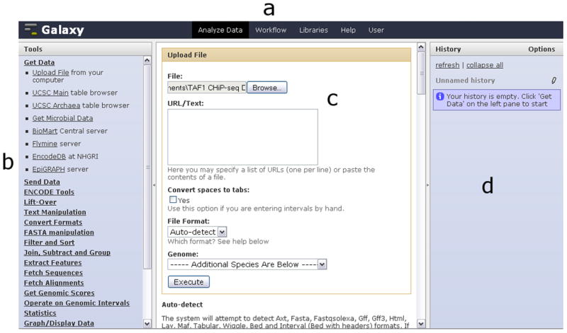
Galaxy’s Analyze Data interface consists of four regions: the masthead (a) at the top, the tool menu (b) on the left-hand side, the work area (c) in the middle and the history panel (d) on the right. The Get Data section has been expanded in the tool menu and the Upload File tool has been selected. In the work area, a local file containing TAF1 CHiP-seq data has been chosen (Basic Protocol 1, step 1); clicking the “Execute” button will cause the data to be uploaded and appear in the history panel.

Basic Protocol 1. An introduction to the Galaxy approach: Finding promoters containing TAF1 binding sites identified from a CHiP-seq experiment

Suppose a CHiP-seq experiment was performed and identified a series of genomic regions that bind TAF1-protein. The next task is to identify a list of genes that contain such sites. This can be easily done with Galaxy in just a few steps. This protocol uses a file arranged by tab-delimited columns, where each column contains information about the genomic positions (“intervals”), as well as name and score data, for TAF1-binding sites from a CHiP-seq experiment. Each row in this file represents an individual TAF1-binding site by listing the chromosome and the start and end positions within that chromosome. Here we assume that the ChIP-seq data has already been processed into putative binding regions, since this procedure is currently very experiment and lab specific. However, as best-practices are defined for performing and evaluating the quality these procedures, appropriate tools will be added to Galaxy.

Materials

• a file containing genomic coordinates for TAF1- binding sites from the CHiP-seq experiment (an example file can be downloaded at http://galaxy.psu.edu/CPMB/TAF1_CHiP.txt). (Kim et al, 2005)

• an internet accessible computer with any modern web browser (Firefox, Safari, Opera, IE).

Steps: (Please note that the items to alter will be stated in the text. If other menus and options are not referenced, leave those settings in their default or existing condition.)

1. Upload the TAF1 CHiP-seq data. Before beginning the analysis the CHiP-seq data needs to be uploaded into Galaxy's workspace (known as a user’s “history” throughout this document).

   1. Go to the public Galaxy site at http://usegalaxy.org.

   2. Click “Get Data”.

   3. Click “Upload file”.

   4. Middle panel of the interface will change and allow selection of the desired file (use the example file that can be downloaded from http://galaxy.psu.edu/CPMB/TAF1_CHiP.txt). Note: It is possible to skip the downloading step and directly upload the data by entering the URL into the paste box, causing Galaxy to fetch the URL contents automatically.

   5. Click “Execute”. The dataset will be uploaded and will appear as dataset #1 within the right panel.

2. Set properties of the TAF1 dataset. To begin the analysis, a number of properties for the CHiP-seq dataset need to be set.

   1. Expand the dataset by clicking on the name of the item in the history list (TAF1_CHiP.txt).

   2. Click “?” next to “database:”. A new interface will appear in the middle panel.

   3. Use the “Database/Build” dropdown to select “Human Mar. 2006 (hg18)”. Click the Save button. The dataset is now designated as originating from the human genome.

   4. Back in the right panel, click the pencil icon. A new interface will appear in the middle.

   5. Use the “New Type” dropdown within the “Change data type” box to select “interval”. The “interval” datatype describes data representing genomic coordinates or “intervals” (chromosomes, start positions and end positions within chromosomes, as well as variable data, for a set of genomic features).

   6. Click the “Save” button immediately below the box. The upper part of the interface will change.

   7. Set “Chrom column”, “Start column” and “End column” to 2, 3 and 4, respectively. Check the “Name” checkbox and select “5” from the adjacent dropdown.

   8. Click the “Save” button immediately below.

   9. The appearance of dataset #1 within the right panel will change -- column headers will appear, and the format will change to “interval”.

3. Upload gene annotations from the UCSC Table Browser (Karolchik et al, 2008 ; Karolchik et al, 2004). To identify which genes' promoters contain the TAF1 binding sites, the gene coordinates must first be uploaded.

   1. Click “Get Data” in the Tools menu list on the left panel.

   2. Click “UCSC Main”. The UCSC Table Browser interface will be displayed in the middle panel.

   3. Because the data is of human annotations, make sure that “clade”, “genome” and “assembly” are set to “Mammal”, “Human” and “Mar. 2006”, respectively.

   4. Set “group” to “Genes and Gene Prediction tracks” and “track” to “RefSeq Genes”.

   5. Select the radio button “genome”.

   6. Make sure “output format” is set to “BED - browser extensible data” and the checkbox by “Send output to Galaxy” is checked. The BED format is a specialized version of the interval format discussed earlier.

   7. Click “get output”. A new interface will appear.

   8. Make sure the “Whole Gene” radio button is selected.

   9. Click “Send query to Galaxy”. At this point a new dataset, #2, will appear in Galaxy's history on the right panel. This dataset contains the genomic positions for all RefSeq genes from the March 2006 human genome assembly.

   10. Rename dataset #2 to “RefSeq” by clicking the pencil icon and typing “RefSeq” in the “Name” field that appears within the center panel. Click the Save button.

4. Transform coordinates of genes into coordinates of putative promoters.

   1. Click “Operate on genomic intervals” in the Tools menu list on the left panel.

   2. Click “Get flanks”. A new interface will appear in the center panel.

   3. Make sure the “Select data” dropdown is set to dataset #2 RefSeq.

   4. Set “Length of the flanking region/s” to “1000”.

   5. Click “Execute”. A new dataset, #3, containing the putative promoters, will appear within the right panel.

   6. Rename dataset #3 to “Promoters” by clicking the pencil icon and typing “Promoters” in the “Name” field that will appear within the center panel. Save.

5. Remove unnecessary columns for dataset #3. Only five columns are needed from this dataset. Galaxy's Cut tool allows the removal of unwanted columns.

   1. Click “Text Manipulation” in the Tools menu list on the left panel.

   2. Click “Cut columns from a table”. A new interface will appear in the center panel.

   3. Type “c1,c2,c3,c4,c6” in the “Cut columns” text box.

   4. Click “Execute”. A new dataset, #4, will appear within the right panel, containing only columns one through four and column six, which correspond to the chromosome, start position, end position, name and strand, respectively, for the calculated promoter regions.

   5. Rename dataset #4 to “Clean Promoters” by clicking the pencil icon and typing “Clean Promoters” in the “Name” field that will appear within the center panel. Save.

   6. Because the Cut tool breaks column assignment, the pencil icon will need to be clicked. A new interface will appear in the middle.

   7. Use the “New Type” dropdown within the “Change data type” box to select “interval”. The “interval” datatype describes data representing genomic coordinates (intervals).

   8. Click the “Save” button immediately below the box. The upper part of the interface will change.

   9. Set “Chrom column”, “Start column” and “End column” to 1, 2 and 3, respectively. Check the “Strand” checkbox and select “5” from the adjacent dropdown. Check the “Name” checkbox and select “4” from adjacent dropdown.

   10. Click the “Save” button immediately below.

   11. The appearance of dataset #4 within the right panel will change -- column headers will appear, and the format will change to “interval”.

6. Identify promoters containing the TAF1 binding sites. Now join the coordinates of TAF1 binding sites from dataset #1 with the coordinates of putative promoters from dataset #4. The Genomic Interval Join Tool matches two separate sets of genomic coordinates (intervals) according to their overlap, creating a single output containing the matched rows.

   1. Click “Operate on Genomic Intervals” in the Tools menu list on the left panel.

   2. Click “Join”. A new interface will appear in the center panel.

   3. Select dataset #4 Clean Promoters from the first dropdown called “Join”.

   4. Select dataset #1 TAF1_CHiP.txt from the second dropdown called “with”.

   5. Make sure the “Return” dropdown is set to “Only records that are joined”.

   6. Click “Execute”. A new dataset, #5, will appear in the right panel. This dataset will list coordinates of putative promoters and TAF1 binding sites side by side as shown in Figure 5.

7. Visualize results of this analysis using the UCSC Genome Browser.

   1. Click “Graph/Display Data” in the Tools menu list on the left panel.

   2. Click “Build custom track”. A new interface will appear in the center panel.

   3. Click “Add new Track” and select dataset #1 TAF1_CHiP.txt from the “Dataset” dropdown.

   4. Type “TAF1” in the “Name” and “Description” boxes. Leave other settings as default.

   5. Click “Add new Track” to create Track 2, and select dataset #4 Clean Promoters from the “Dataset” dropdown.

   6. Type “Promoters” in the “Name” and “Description” boxes. Set the color to Blue.

   7. Click “Add new Track” to create Track 3 and select dataset #5 from the “Dataset” dropdown.

   8. Type “Overlap” in the “Name” and “Description” boxes. Set the color to Purple.

   9. Click “Execute”. A new dataset, #6 Build custom track on data 5, data 4, and data 1, will appear within the right panel.

   10. Once dataset #6 becomes green in the History panel list, click on its name and then click the “display at UCSC main” link. The browser will open a new window or a tab with the UCSC Genome Browser interface displaying datasets 1, 4 and 5 as custom tracks.

Figure 5.

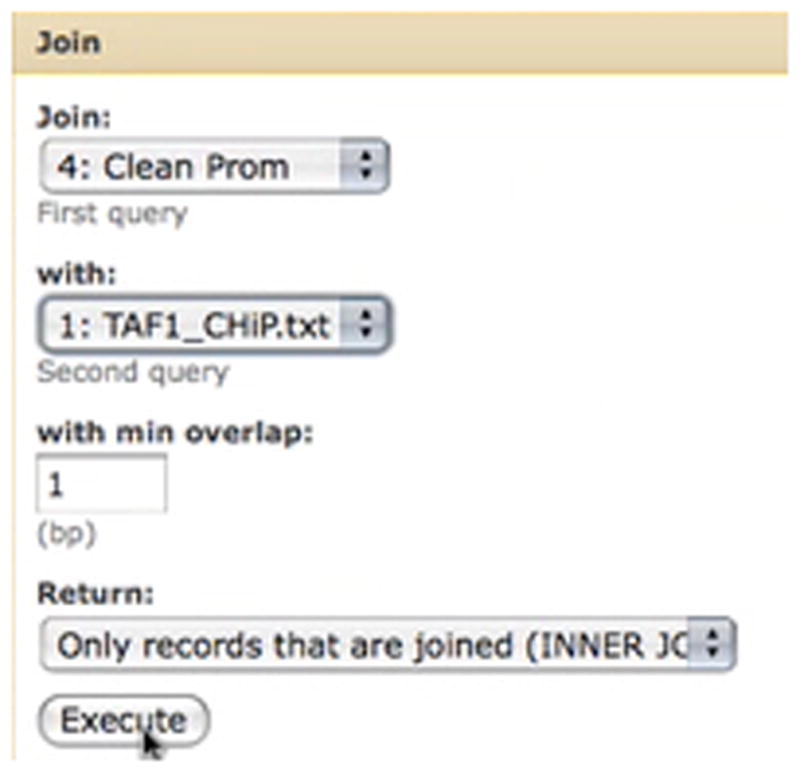
The Join tool is used to create a dataset which contains the coordinates of putative promoters and TAF1 binding sites side by side (Basic Protocol 1, step 6).

Basic Protocol 2. Combining and filtering genome annotations: Finding Exons with the highest number of nucleotide polymorphisms

The objective of this protocol is to demonstrate joining, grouping, sorting, and filtering of genomic annotations in Galaxy. To explore these features using real data an illustrative example will be used: identification of exons containing the largest number of single nucleotide polymorphisms (SNPs).

Materials

• an internet accessible computer with any modern web browser (Firefox, Safari, Opera, IE).

Steps: (Please note that it is beneficial to clear the current history and start re-numbering from 1 by accessing the History Options and selecting “Create a new empty history”. It simplifies following with the numbered steps.)

1. Upload exon annotations from the UCSC Table Browser.

   1. Click “Get Data” in the Tools menu list on the left panel.

   2. Click “UCSC Main”. The UCSC Table Browser interface will be displayed in the middle panel.

   3. Because the data of interest are human annotations make sure that “clade”, “genome” and “assembly” are set to “Mammal”, “Human” and “Mar. 2006”, respectively.

   4. Set “group” to “Genes and Gene Prediction tracks” and “track” to “UCSC Genes”.

   5. Select the radio button “position” and type “chr22” within the adjacent text box. This will limit the annotations to the entirety of chromosome 22.

   6. Make sure “output format” is set to “BED - browser extensible data” and the checkbox by “Set output to Galaxy” is checked. The BED format is a specialized version of the interval format discussed earlier; it contains the information required to represent a genomic position.

   7. Click “get output”. A new interface will appear.

   8. Make sure the “Coding Exons” radio button is selected in the “Create one BED record per:” area. The genes on chromosome 22 will be divided into coding exons, with each exon having its own set of genomic intervals.

   9. Click “Send query to Galaxy”. At this point a new dataset, #1, will appear in Galaxy's history on the right panel. A query in the queue will be indicated by a gray box, a running query will be yellow, and a completed query will have a green box.

   10. When the query has completed, rename dataset #1 to “exons” by clicking the pencil icon and typing “exons” in the “Name” field that will appear within the center panel. Click the Save button.

2. Upload SNP coordinates.

   1. Click “Get Data” from the Tools menu list on the left panel.

   2. Click “UCSC Main”. The UCSC Table Browser interface will be displayed in the middle panel.

   3. Because the data of interest are human annotations, make sure that “clade”, “genome” and “assembly” are set to “Mammal”, “Human” and “Mar. 2006”, respectively.

   4. Set “group” to “Variation and Repeats” and “track” to “SNPs (129)”.

   5. Select the radio button “position” and type “chr22” within the adjacent text box.

   6. Make sure “output format” is set to “BED - browser extensible data” and a checkbox by “Set output to Galaxy” is checked.

   7. Click “get output”. A new interface will appear.

   8. Make sure the “Whole Gene” radio button is selected in the “Create one BED record per:” area.

   9. Click “Send query to Galaxy”. At this point, a new dataset, #2, will appear in Galaxy's history in the right panel.

   10. When the query has completed, rename dataset #2 to “snps” by clicking the pencil icon and typing “snps” in the “Name” field that will appear within the center panel. Save.

3. Join coordinates of exons with coordinates of SNPs to identify those exons that contain SNPs.

   1. Click “Operate on Genomic Intervals” in the Tools menu list on the left panel.

   2. Click “Join” in the Operate submenu. A new interface will appear in the center panel.

   3. Select dataset #1 exons from the first dropdown called “Join”.

   4. Select dataset #2 snps from the second dropdown called “with”.

   5. Make sure the “Return” dropdown is set to “Only records that are joined (INNER JOIN)”.

   6. Click the “Execute” button. A new dataset, #3 Join on data 2 and data 1, will appear in the right panel. This dataset will list coordinates of exons and SNPs side by side as shown in Figure 7. The data can by examined by clicking on the name.

4. Count the number of SNPs per exon using the Group tool. In Figure 7, it is seen that if an exon contains multiple SNPs its name is repeated. It is possible to take advantage of this by using the Group tool. By counting the number of times each exon's name appears within dataset #3, the number of SNPs within that exon will be obtained.

   1. Click “Join, Subtract, and Group” from the Tools menu list on the left panel.

   2. Click “Group”. A new interface will appear in the center panel.

   3. Set the “Select data:” dropdown to dataset #3 Join on data 2 and data 1.

   4. Set “Group by column” to “c4”, as this column contains exon identifiers.

   5. Click the “Add new operation” button. A new section of interface named “Operation 1” will appear below.

   6. Within the new interface section, set “Type” to “Count” and “On column” to “c4”.

   7. Click the “Execute” button. A new dataset, #4 Group on data 3, will appear in the right panel. It will contain two columns: (1) exon id and (2) SNP count.

5. Sort exon by SNP count. To see the highest possible number of SNPs per exon in this dataset, sort the dataset from the previous step.

   1. Click “Filter and Sort” from the Tools menu list on the left panel.

   2. Click “Sort”. A new interface will appear in the center panel.

   3. Set “Sort Query” to dataset #4 Group on data 3.

   4. Set “on column” to “c2” (the SNP count calculated above).

   5. Click “Execute”. Dataset #5 Sort on data 4 will appear in the history panel.

   6. Click on the eye icon to see which exons have the highest SNP count.

6. Restrict dataset #5 to exons that have ten or more SNPs.

   1. Click “Filter and Sort” from the Tools menu list on the left panel.

   2. Click “Filter”.

   3. Set “Filter” to dataset #5 Sort on data 4.

   4. Set “With following condition” to “c2 >= 10” (without the quotes). This is because column 2 (c2) contains the count of SNPs per exon; only rows in which the contents of column two is greater-than or equal-to ten will be kept.

   5. Click “Execute”. Dataset #6 Filter on data 5 will appear in the history panel.

7. Restore genomic location for exons containing ten or more SNPs. The previous step has produced a list of exons containing ten or more SNPs, however, information about their genomic position, strand orientation, etc has been lost. Because dataset #6 contains the exon identifier field, it can be used to restore genomic context information by joining with dataset #1. The Join two Queries tool is different than the Genomic Operations Join which was used earlier; this tool matches two separate datasets by matching column contents between any tab-delimited dataset (including interval datasets).

   1. Click “Join, Subtract, and Group” from the Tools menu list on the left panel.

   2. Click “Join two Queries”. A new interface will appear within the center panel.

   3. Set “Join” to dataset #1 exons.

   4. Set “Using column” to “c4” as this column contains exon identifiers in dataset #1.

   5. Set “with” to dataset #6 Filter on data 5.

   6. Set “and column” to “c1” as this column contains exon identifiers in dataset #6.

   7. Click “Execute”. Dataset #7 Join two Queries on data 6 and data 1 will appear within the history panel on the right. It contains full genomic context information about exons containing ten or more SNPs in chromosome 22.

8. Visualize dataset #7 Join two Queries on data 6 and data 1 in UCSC Genome Browser.

   1. Go to the right (history) panel and expand dataset #7 by clicking on the name of the dataset.

   2. Click the “display at UCSC main” link. A new browser tab (or window) will open dataset #7 within the UCSC Genome Browser. The query will be displayed as a track called “User Supplied Track”. Access to menu control of this track is available in the menus area below, and the track will be available in the UCSC Table Browser for further query and manipulation.

9. To save the analysis and share it with colleagues continue on to Support Protocol 2.1

Figure 7.

A dataset containing exons and overlapping SNPs has been created (Basic Protocol 2, step 4) using the Join tool and has been displayed in the middle panel by clicking on the eye icon next to dataset 3. A red rectangle has been drawn around an exon which overlaps with 4 SNPs.

Support Protocol 2.1. Saving results in Galaxy and sharing data with others

How can researchers ensure that the analyses they have just conducted are safely stored and that they are able to go back to them at anytime? They will need to create a free account within Galaxy. This is the only requirement to save analyses. The protocol below explains this and also introduces sharing analyses with colleagues.

Materials

• an internet accessible computer with any modern web browser (Firefox, Safari, Opera, IE).

• completed protocols – results of Basic Protocol 2.

• A Galaxy account (created by clicking “Register” in the Galaxy interface). Histories must be linked to a user to be stored and shared.

Steps

1. Rename the history. All histories are given the default name “unnamed”, which is obviously not very descriptive. This is easily changed by following the steps below.

   1. Click the pencil icon immediately above the history items (on a lavender background). A text box will appear to the left of the pencil.

   2. Type “Exons and SNPs” in the textbox and hit the Enter key or return key on the keyboard.

2. Click the “Options” button above the history panel. A list of history actions will appear in the middle panel.

3. Click the “Share current history” link

4. Enter the e-mail address of an existing Galaxy user and click “Submit”. This history is now shared.

Basic Protocol 3. Generating a workflow from a history in Galaxy

Protocols 1 and 2 demonstrate interactive analysis in Galaxy, the result is a “history” which documents each step of an analysis. Galaxy also allows the construction of reusable multi-step analysis “workflows”. In this protocol, the creation of a workflow from an existing analysis history is demonstrated.

Materials

• an internet accessible computer with any modern web browser (Firefox, Safari, Opera, IE).

• completed protocols – the history that was created by following Basic Protocol 2.

• A Galaxy account (created by clicking “Register” in the Galaxy interface). All workflow in Galaxy requires the user to be logged in with an account.

Steps

1. Ensure a non-empty history is loaded (for this example, the history resulting from the completion of Basic Protocol 2 is used).

2. In the header of the History panel (top-right of the Galaxy analysis interface) click “Options”. This will load a menu of options, which apply to the current history, in the center panel.

3. In the center panel, click “Construct workflow from the current history”. This will load a list of the actions (tool runs) which generated each dataset in the current history. A subset of tools can be selected by clicking the checkboxes on this page (e.g. if more than one analysis has been performed in the current history, but a workflow is only to be created from one of them). Certain tools cannot be used in workflows (including most external data sources), in these cases the dataset can be treated as an input to the workflow. Here, a workflow is constructed from the entire history, so do not change any checkboxes.

4. Provide a name for the new workflow by entering a name of choice in the text box underneath the label “Workflow name”.

5. Click the “Create Workflow” button to create the new workflow; a message will be displayed in the center panel confirming that the workflow was created.

Support Protocol 3.1. Modify a parameter of the workflow in Galaxy

After constructing a workflow from an existing analysis, the Workflow Editor can be used to modify tool parameters (or even add and remove steps).

Materials

• an internet accessible computer with any modern web browser (Firefox, Safari, Opera, IE).

• completed protocols – the workflow that was created by following Basic Protocol 3.

Steps

1. Move from the “Analyze Data” view to the “Workflow” view by clicking “Workflow” in the top panel of the Galaxy interface. The workflow view provides access to all workflow management functionality (editing, sharing, etc).

2. Load the workflow in the workflow editor.

   1. Click the triangle next to the name of the workflow that was just created.

   2. Select “edit” from the menu that appears.

3. Drag the workflow canvas (center panel) until the box labeled “Filter” is visible. Each box in the canvas represents a step of the workflow. The canvas viewport can be moved by dragging the background or by dragging the blue box in the overview panel (bottom right).

4. Click the box for the “Filter” step in the canvas, it will be outlined in blue, showing that it is the active step, and a form showing the tool parameters will appear in the right panel.

5. Modify this step to filter regions with 50 or more SNPs by entering the text “c2 >= 50” (without the quotes) in the textbox under the label “With the following condition” and clicking “Save” in the right panel.

6. Save the changes to the workflow by clicking “Save” in the header of the center panel. It is important to save both the changes to the step and the changed step to the workflow.

Support Protocol 3.2 Running workflows with Galaxy

Once a workflow has been constructed, it can be run in the analysis view just like any other tool in Galaxy.

Materials

• an internet accessible computer with any modern web browser (Firefox, Safari, Opera, IE).

• completed protocols – the workflow that was saved in Basic Protocol 3.

Steps

1. Return to the Analyze Data view by clicking “Analyze Data” in the top panel.

2. Create a new empty history in which to store the result of running the workflow.

   1. In the header of the History panel (top-right of the Galaxy analysis interface) click “Options”.

   2. In the center panel click “Create a new empty history”

3. Get exon and SNP annotations for human chromosome X from the UCSC Table Browser.

   1. Follow Steps 1 and 2 of Basic Protocol 2; however, enter “chrX” instead of “chr22”.

4. Click “Workflow” at the bottom of the tool menu (left panel), then click “All workflows” in the list of options that appears.

5. In the center panel, click the name of the workflow created above in Basic Protocol 3. This will load the workflow in the center panel with prompts for parameters that need values.

6. Under “Step 1: Input Dataset” select the second item in the history (the SNPs).

7. Under “Step 2: Input Dataset” select the first item in the history (the exons).

8. Click “Run Workflow” at the bottom of the form in the center panel. A message will be displayed confirming that the workflow has been run, and the datasets for each workflow step will be added to the history (in the 'queued' state). At this point, the workflow is running, and each step will execute once the data it requires has been generated by previous steps. The box surrounding the dataset will change color based upon its state as the steps progress: a query in the queue will be indicated by a gray box, a running query will be yellow and a completed query will have a green box.

Support Protocol 3.3 Sharing workflows with Galaxy

Galaxy allows researchers to share workflows with others. Workflows can either shared with a specific Galaxy user, or made publicly accessible by a special link.

Materials

• an internet accessible computer with any modern web browser (Firefox, Safari, Opera, IE).

• completed protocols – the workflow that was created using Basic Protocol 3

Steps

1. Move from the “Analyze Data” view to the “Workflow” view by clicking “Workflow” in the top panel of the Galaxy interface. This is located in the dark blue navigation banner across the top of the interface.

2. Click the triangle next to the name of the workflow to be shared and select “Sharing”.

3. To allow others to import the workflow by following a link.

   1. Click “Enable import via link”.

   2. Copy the link that is displayed.

   3. Provide the link to anyone wanting to access the workflow (e.g. via email, including in a publication, etc).

4. To share the workflow only with a specific user.

   1. Click “Share with another user”.

   2. Enter the email address of a user to share with in the textbox.

   3. Click “Share”. If the email address corresponds to another Galaxy user, they will now see the workflow in their workflow view.

Basic Protocol 4. Generating workflows from scratch with Galaxy

In addition to creating workflows from existing histories, Galaxy allows the creation of a workflow from scratch. In this protocol a simple workflow that finds the 50 longest intervals from a dataset in a 6 column BED file is constructed. The BED format is a specialized version of the interval format discussed earlier; it contains the information required to represent a genomic position. A 6 column BED file contains the chromosome, start position in the chromosome, end position in the chromosome, name, score, and strand for a set of genomic positions. Insert Figure 9 here.

Figure 9.

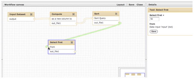
The Workflow Editor allows users to click to add new tools and connect the output of one tool to the input of another by simple clicking and dragging. The output of the Sort tool is being connected to the Select first tool (Basic Protocol 4, step 9), as is shown by the green rope; when the mouse button is released, the connection will be created and the rope will become white.

Materials

• an internet accessible computer with any modern web browser (Firefox, Safari, Opera, IE).

• A Galaxy account (created by clicking “Register” in the Galaxy interface). All workflow in Galaxy requires the user to be logged in with an account.

Steps

1. Move from the “Analyze Data” view to the “Workflow” view by clicking “Workflow” in the top panel of the Galaxy interface.

2. Create a new empty workflow.

   1. Click the “Add a new workflow” button near the top.

   2. Enter a name for the workflow in the text box under the label “Workflow name”.

   3. Click “Create”.

3. Load the (empty) workflow in the workflow editor.

   1. Click the triangle next to the name of the workflow that was just created.

   2. Select “edit” from the menu that appears.

4. Add an input dataset to the workflow.

   1. In the right panel, click “Inputs” from the Tools menu on the left,and then select “Input Dataset”. A box (called a “node”) will appear in the middle of the center panel (called the “Workflow canvas”).

   2. Move the node representing the input dataset to the top-left of the editor canvas by dragging it by the title.

5. Add a step to the workflow to compute the length of each interval in the input dataset.

   1. Click “Text Manipulation” from the Tools menu on the left and then select “Compute” in the left panel.

   2. Drag the newly created node up and place it to the right of “Input Dataset” (leaving some space). Note: its also possible to click “Layout” in the top of the center panel to automatically organize nodes in the canvas.

6. Create a connection between the input dataset and the Compute node. Outputs of a node are represented by circled arrowheads overlapping the right edge of a node, while data inputs are circled arrowheads overlapping the left edge of a node. Connections are made by dragging.

   1. Click and hold the arrowhead next to the label “output” in the “Input Dataset” node.

   2. Drag the mouse, a curve should follow the mouse pointer.

   3. Drag over the arrowhead next to the label “as a new column to” in the “Compute” node. The curve should turn green indicating that the connection is valid (datatypes are compatible).

   4. Release the mouse to make the connection.

7. Add a step to the workflow to sort the intervals by length.

   1. Click “Filter and Sort” from the Tools menu on the left and then choose “Sort” in the left panel.

   2. Position the new node to the right of the previously created nodes by dragging.

   3. Create a connection between the output labels “out_file1” of “Compute” with the input “Sort query” of “Sort”.

8. Add a step to the workflow to select the longest intervals.

   1. Click “Text Manipulation” from the Tools menu on the left and then “Select first lines from a Query in the left panel.

   2. Position the new node to the right of the previously created nodes by dragging.

   3. Create a connection between the output labels “out_file1” of “Sort” with the input “from” of “Select first”.

9. Edit the parameters of the “Compute” step to calculate interval length.

   1. Click the “Compute” node in the canvas. In the right panel a new form will appear. The parameters for this workflow action can be edited using the text boxes and menu choices.

   2. In the text box under “on column” enter “c3 - c2” (without the quotes) to subtract column 2 (start position) from column 3 (end position). Note that this may already be the default value for this field.

   3. Click the “Save” button in the right panel to validate and save the parameters.

10. Edit the parameters of the “Sort” step to sort on the correct column.

    1. Click the “Sort” node in the canvas. Its action options will appear in the right panel form.

    2. In the text box under “on column” enter “7”. Since the data is a 6 column BED file, the length computed in the “Compute” step will have been stored in column 7.

    3. Click “Save” in the right panel to validate and save the parameters.

11. Edit the parameters of the “Select first” step to select the first 50 intervals.

    1. Click the “Select first” node in the canvas. Its action options will appear in the right panel.

    2. In the text box under “Select first” enter “50”.

    3. Click “Save” in the right panel to validate and save the parameters.

12. Click the “Save” button in the title bar header of the center workflow canvas panel to save the workflow as a whole.

13. Click “Close” in the header of the workflow canvas panel to return to the workflow list. This workflow can now be run in the same fashion as described in Support protocol 3.2.

Basic Protocol 5. Extracting Sequences and alignments with Galaxy: A SNPs in exons example

This protocol demonstrates how Galaxy is used to extract genomic sequences and multiple species alignments corresponding to regions of interest. It starts with the data that was generated in Basic Protocol 2, where human coding exons with high SNP counts were found. Two types of data will be extracted for these regions: the genomic sequence of each region, and pieces of a whole genome alignment between human and other species overlapping these regions. Because the whole genome alignment used here (produced by Multiz, a local aligner) is fragmented into pieces, these pieces will then be projected back onto the regions of interest (exons) to facilitate per-exon analysis of the alignments (the result is sometimes called a “pseudo-global” alignment. This protocol is a brief illustration of how easily the often tricky manipulation of these files is with Galaxy.

Materials

• an internet accessible computer with any modern web browser (Firefox, Safari, Opera, IE).

• completed protocols – the completed and saved the history that was created by following Basic Protocol 2 and Support Protocol 2.1.

Steps

1. Return to the main Galaxy interface by going to http://usegalaxy.org.

2. Load the history created in Basic Protocol 2:

   1. Click “Options”, located at the top right of the History Panel; History Options will appear in the middle panel.

   2. Click “List previously stored histories”; all histories associated with the current user will be displayed.

   3. Click on the history that was saved earlier as “Exons and SNPs”.

3. The history panel will refresh with the selected history, which should contain 7 steps. Dataset #7 Join two Queries on data 6 and data 1 contains the genomic coordinates of the exons of interest.

4. Extract Genomic DNA corresponding to each of the exons.

   1. In the Tools panel, click to expand the “Fetch Sequences” menu.

   2. Click the item titled “Extract Genomic DNA”; the tool’s interface will appear in the center.

   3. Select dataset #7 Join two Queries on data 6 and data 1 as the input query.

   4. Set output datatype to “FASTA”.

   5. Click “Execute”.

5. When the query finishes, a dataset containing one human sequence for each of the exons (total of 109 sequences) called “Extract Genomic DNA on data 7” is created. This dataset contains the human genomic DNA corresponding to each of the 109 exons in FASTA format, a very common format for storing multiple named sequences.

6. Extract multiple species alignment blocks for each of the human exon locations.

   1. In the Tools panel, click to expand the “Fetch Alignments” menu.

   2. Click the item titled “Extract MAF blocks”; the tool’s interface will appear in the center. MAF stands for multiple alignment format, a standard format for large alignments of multiple genomes. A genome-wide local alignment of multiple genomes consists of many regions of high scoring alignment called “blocks”.

   3. Select dataset #7 Join two Queries on data 6 and data 1 as the interval source.

   4. Set MAF Source to “Locally Cached Alignments”.

   5. Under Choose alignments, set “5-way multiZ” using the pulldown menu. This alignment contains 5 different mammals including human. Most of the locally cached multiple-species whole-genome alignments available in Galaxy were generated using the UCSC/Penn State Bioinformatics comparative genomic alignment pipeline; these original source alignments are available from the UCSC download site.

   6. Click the “Select All” button to choose to extract all species.

   7. Click the “Execute” button.

7. A new history item is created, #9 Extract MAF blocks on data 7, which contains the portions of the source alignment which overlap with the exon regions. For the 109 regions, 387 alignment blocks were retrieved, which is due to multiple local alignment blocks overlapping individual exons. Thus, the resulting dataset contains every local alignment block overlapping an exon, trimmed to just include the portion of the alignment that overlapped. This dataset is useful for examining the conservation of exons in aggregate, however the relationship between exons and alignments has been lost.

8. Create one projected alignment per human exon.

   1. In the Tools panel, ensure that the “Fetch Alignments” menu is still expanded.

   2. Click the item titled “Stitch MAF blocks”; the tool’s interface will appear in the center.

   3. Select dataset #7 Join two Queries on data 6 and data 1 as the input intervals.

   4. Set MAF Source to “Alignments in Your History”.

   5. Select dataset #9 Extract MAF blocks on data 7 for MAF File.

   6. Click the “Select All” button to choose to extract all species.

   7. Click “Execute”.

9. A new history item is created, #10 Stitch MAF blocks on data 7 and data 9, which contains one alignment block for each of the human exons, with regions where no alignment was found represented as gaps (-). Click the eye icon to examine the data in the center panel. The projected alignment is in FASTA format, suitable for downstream analysis in most phylogenetic software packages, including those available in Galaxy. For 109 regions, 545 FASTA sequences (109 regions each with sequences for 5 species) were generated in 109 alignment blocks.

Commentary

Galaxy successfully bridges the gap between data collection and analysis. The public Galaxy server allows researchers across the globe to perform computationally intensive, large-scale analyses with the only equipment requirement consisting of an internet-connected web browser. Users are not required to delve into the intricacies of how to execute a large collection of unrelated programs, but instead have access to a unified point and click interface. Galaxy provides both experimental biologists and their computational brethren with a framework to facilitate truly reproducible cutting edge science.

The protocols contained within this unit offer only a glimpse of possible analyses and tool functionality. The text contained here should only be considered an introduction to performing complex analysis with Galaxy. New datasets, tools, and features will be added regularly. Some new menu choices may arise or move. In addition to the screencasts that accompany these protocols; many more screencasts that demonstrate additional functionality are available at http://galaxycast.org and others will be added over time.

Transparency and reproducibility

Open and transparent research is essential to the process of science. Research papers cannot be published without making the protocols and generated experimental data publically available. Unfortunately, the same standards are often not applied to computational analysis. When analysis is performed within Galaxy, every detail is preserved in the “history” and can be inspected later. These histories can be shared or published, and can be reproduced (with or without modification) through the workflow system. Thus, without additional effort on the part of the user, Galaxy facilitates greater transparency and reproducibility of computational analyses.

Collaboration

While the scope of this unit is limited to introducing a user to performing data analysis with the public Galaxy server, Galaxy is also an excellent resource for collaborative analysis. Because it is web-based, collaborators at different locations can easily and rapidly share data and analysis. In particular, Galaxy’s library system provides for sharing of datasets within research groups, with access controls and version histories.

Research groups that have their own collections of analysis scripts and binaries will find it worthwhile to download the open source framework, integrate their unique tools, and maintain a private server (a “Galaxy instance”) for lab members to work on their projects. A local Galaxy server makes collaborations between computational and experimental researchers more efficient, since new analysis tools can be effortlessly made available to colleagues, allowing programmers to focus on method development. Although beyond the scope of this introduction to the user interface, documentation and assistance for programmers is also available on the Galaxy site.

The Galaxy Framework is easily downloaded, quickly configured and effortlessly deployed. Although written in Python, no knowledge of the Python programming language is required to deploy or maintain a personal Galaxy instance. This facilitates local development of new tools, the creation of new Galaxy instances with custom toolsets, and secure private Galaxy instances for analyzing protected data (e.g., genotype data obtained in clinical setting). To download the Galaxy Framework and view detailed installation documentation visit http://getgalaxy.org.

Help and feedback

Galaxy is under constant development and is improved based upon user suggestions. Extensive help is available in the form of screencasts as well as active public mailing lists, where both experimentalists and computationalists can request and receive advice. Discussion of feature requests is also encouraged. For links to these resources and to use Galaxy, visit http://galaxyproject.org.

Figure 2.

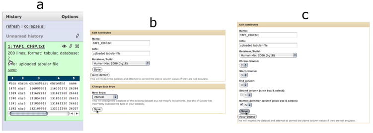
To change the properties of a dataset (Basic Protocol 1, step 2), click on the question mark (or the pencil icon) associated with our dataset in the history panel (a). This causes the Edit Attributes page to appear in the center panel (b) where the datatype has been changed from tabular to interval; clicking “Save” causes the page to refresh allowing additional interval-specific information to be set (c).

Figure 3.

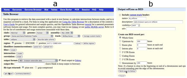
The UCSC Table browser tool has been selected and its interface (a) appears in the center panel; the refGene table has been selected and the output is marked to be sent to Galaxy (Basic Protocol 1, step 3). Once output style is specified (b), clicking “Send query to Galaxy” will create a new dataset in the history panel.

Figure 4.

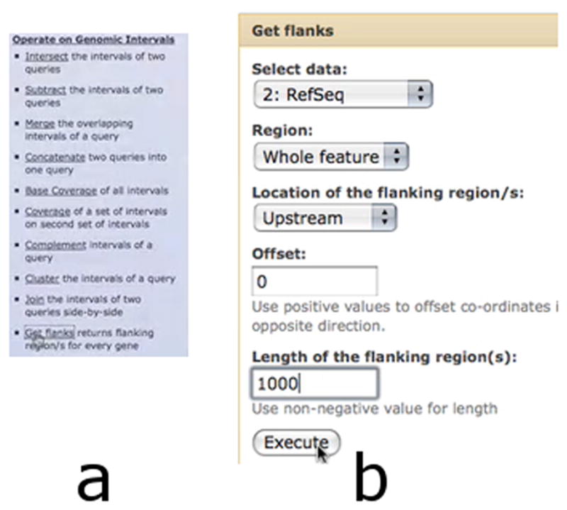
Selecting the Get flanks tool (Basic Protocol 1, step 4) from the Operate on Genomic Intervals Section (a) allows the creation of new data containing the region 1000 nucleotides upstream of our RefSeq genes (b).

Figure 6.

The Build custom track tool (Basic Protocol 1, step 7) allows the user to design a custom track suitable for display at the UCSC Genome Browser (d) by progressively adding new tracks containing varying datasets (a-c).

Figure 8.

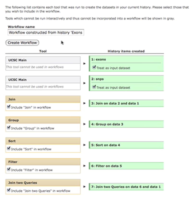
In order to create a workflow from an existing history (Basic Protocol 3), the user needs to make sure that they are logged in and then select “History Options” and click “Construct workflow from the current history”. A new workflow will be populated from the current history as shown; the workflow can now be renamed and created.

Figure 10.

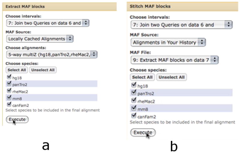
Several options exist for obtaining multi-species alignments (Basic Protocol 5). The Extract MAF blocks tool (a) creates a MAF dataset which contains only the trimmed alignment blocks which overlap a specified set of intervals. The Stitch MAF blocks tool (b) creates a FASTA file which contains a single alignment block per provided interval.

Screencasts.

1. Finding promoters containing TAF1 binding sites identified from a CHiP-seq experiment

http://galaxycast.org/cpmb-2009-1

Suppose you performed a CHiP-seq experiment and identified a series of genomic regions that bind TAF1-protein. You now need to identify a list of genes that contain such sites. This can be easily done with Galaxy in just a few steps. To run this example yourself you will need a file containing genomic coordinates for TAF1- binding sites from the CHiP-seq experiment (an example file can be downloaded from http://galaxy.psu.edu/CPMB/TAF1_CHiP.txt).

2. Finding Exons with the highest number of nucleotide polymorphisms

http://galaxycast.org/cpmb-2009-2

In this protocol we will work with two sets of genomic features: exon coordinates and single nucleotide polymorphism (SNP) coordinates. The objective will be to identify exons that contain the highest number of SNPs. Even if you are not particularly interested in exons and SNPs, we encourage you to follow along as the real goal of this protocol is to introduce you to joining, grouping, sorting, and filtering in Galaxy.

3. Saving your results and sharing data with others

http://galaxycast.org/cpmb-2009-3

How can you ensure that the analyses you have just conducted are safely stored and that you are able to go back to them at anytime? You will need to create a free account within Galaxy. This is the only requirement to save your analyses. The protocol below explains this and also introduces sharing analyses with colleagues.

4. Generating a workflow from a history

http://galaxycast.org/cpmb-2009-4

Screencasts 1 and 2 within this series demonstrate interactive analysis in Galaxy, the result is a history which documents each step of an analysis. Galaxy also allows you to construct reusable multi-step analysis workflows. In this protocol, we will demonstrate the creation of a workflow from an existing analysis history.

5. Generating workflows from scratch

http://galaxycast.org/cpmb-2009-5

In addition to creating workflows from existing histories, Galaxy allows us to create a workflow from scratch. In this protocol we will construct a simple workflow that finds the 50 longest intervals from a dataset in a 6 column BED file.

6. Extracting Sequences and alignments: A SNPs in exons example

http://galaxycast.org/cpmb-2009-6

Here we demonstrate how Galaxy is used to extract genomic sequences and multiple species alignments corresponding to regions of interest. In this protocol, we start with the data that we generated in Screencast 2, where we found human coding exons with high SNP counts. We will extract genomic sequences for our regions in FASTA format as well as obtain corresponding alignment blocks from multiple species whole genome alignments in their native format and also create a pseudo-global alignment in FASTA format, which is suitable for use in existing analysis software.

Literature cited

- Karolchik D, Kuhn RM, Baertsch R, Barber GP, Clawson H, Diekhans M, Giardine B, Harte RA, Hinrichs AS, Hsu F, Miller W, Pedersen JS, Pohl A, Raney BJ, Rhead B, Rosenbloom KR, Smith KE, Stanke M, Thakkapallayil A, Trumbower H, Wang T, Zweig AS, Haussler D, Kent WJ. The UCSC Genome Browser Database: 2008 update. Nucleic Acids Res. 2008 Jan;36:D773–9. doi: 10.1093/nar/gkm966. [DOI] [PMC free article] [PubMed] [Google Scholar]
- Karolchik D, Hinrichs AS, Furey TS, Roskin KM, Sugnet CW, Haussler D, Kent WJ. The UCSC Table Browser data retrieval tool. Nucleic Acids Res. 2004 Jan 1;32(Database issue):D493–6. doi: 10.1093/nar/gkh103. [DOI] [PMC free article] [PubMed] [Google Scholar]
- Kim TH, Barrera LO, Zheng M, Qu C, Singer MA, Richmond TA, Wu Y, Green RD, Ren B. A high-resolution map of active promoters in the human genome. Nature. 2005 Aug 11;436:876–80. doi: 10.1038/nature03877. [DOI] [PMC free article] [PubMed] [Google Scholar]
- Taylor J, Schenck I, Blankenberg D, Nekrutenko A. Using galaxy to perform large-scale interactive data analyses. Curr Protoc Bioinformatics. 2007 Sep;Chapter 10(Unit 10.5) doi: 10.1002/0471250953.bi1005s19. [DOI] [PMC free article] [PubMed] [Google Scholar]