

Abstract
Rationale
Previously we reported methods to estimate peak breath alcohol concentrations (BrAC) from transdermal alcohol concentrations (TAC) under conditions where alcohol consumption was controlled to produce similar BrAC levels in both sexes.
Objective
This study characterized differences in the relationship between BrAC and TAC as a function of sex, and developed a model to predict peak BrAC that accounts for known sex differences in peak BrAC.
Methods
TAC and BrAC were monitored during the consumption of a varying number of beers on different days. Both men (n = 11) and women (n = 10) consumed 1, 2, 3, 4, and 5 beers at the same rate in a two-hour period. Sex and sex-related variables were considered for inclusion in a multilevel-model to develop an equation to estimate peak BrAC levels from TAC.
Results
While peak BrAC levels were significantly higher in women than men, sex differences were not significant in observed TAC levels. This lack of correspondence was evidenced by significant sex differences in the relationship between peak TAC and peak BrAC. The best model to estimate peak BrAC accounted for sex-related differences by including peak TAC, time-to-peak TAC, and sex. This model was further validated using previously collected data.
Conclusions
The relationship between peak TAC and actual peak BrAC differs between men and women, and these differences can be accounted for in a statistical model to better estimate peak BrAC. Further studies are required to extend these estimates of peak BrAC to the outpatient environment where naturalistic drinking occurs.
Keywords: Transdermal alcohol monitoring, Binge drinking, Alcohol abuse, Breath and blood alcohol concentration
Introduction
Excessive alcohol consumption is responsible for more than 79,000 deaths annually (CDC 2011) and is the third-leading preventable cause of death in the United States (Mokdad et al. 2004). Unhealthy levels of alcohol consumption increase the risk for health problems (Rehm et al. 2003a; Rehm et al. 2003b) and are associated with significant behavioral and economic consequences (Bouchery et al. 2011; CDC 2011). NIAAA defines “unhealthy” levels as ≥4 drinks for women and ≥5 drinks for men during a single day. “Binge” drinking has been identified as particularly problematic and is defined as heavy drinking (4 standard drinks for women and 5 for men) within a 2-hour period resulting in intoxicating levels putting individuals at serious risk of medical, legal, and psychosocial problems (CDC, 2012; NIAAA, 2004; NIAAA, 2014; Wechsler and Nelson, 2001). A recent analysis (Bouchery et al. 2011) estimated that the cost of alcohol abuse was $223.5 billion in 2006. Consequently, sensitive and specific measures of alcohol consumption are needed to better understand the etiology of unhealthy levels of alcohol consumption to develop effective treatment and intervention strategies for reducing this dangerous behavior.
An accurate picture of drinking patterns among heavy drinkers is needed to make treatments and interventions for excessive drinking more effective. Despite adequate reliability and validity in research settings (Del Boca and Darkes2003), self-reported alcohol consumption still tends to be under-estimated in real-world settings (de Visser and Birch 2012; Devos-Comby and Lange 2008; Kerr and Stockwell 2012; White et al. 2003). The accuracy of self-reported drinking may be especially compromised when large quantities (i.e., binge) of alcohol are consumed (Sobell and Sobell 2003). Furthermore, alcohol concentrations vary across beverage types, leading people to underestimate how much actual alcohol they have consumed (Devos-Comby and Lange 2008; White et al. 2003).
Because of these inaccuracies, objective measures of alcohol consumption are required. Although several alcohol biomarkers have been developed, they either: (1) have short half-lives [e.g., breath and blood alcohol concentrations (hours), urinary ethyl glucuronide, urinary ethyl sulfate (days)] which limit their window of detection; (2) are non-specific (e.g., carbohydrate deficient transferrin and γ-glutamyl transferase), possibly resulting in false positive results; or (3) need to be better characterized (e.g., phosphatidylethanol; Hahn et al. 2011; Helander et al. 2012; Javors and Johnson 2003; Marques et al. 2010; Marques 2012). Transdermal alcohol monitoring is the direct electrochemical detection of the small amount (approximately1%) of ingested alcohol that is excreted through the skin (Swift, 2003). The transdermal alcohol concentration (TAC) is the concentration of alcohol measured in the skin surface water vapor, or insensible perspiration (Swift, 2003; Swift and Swette, 1992). Transdermal alcohol monitoring is a noninvasive method that continuously gathers data about an individual’s drinking behavior in real time (Ayala et al. 2009; Barnett et al. 2011; Dougherty et al. 2012; Leffingwell et al. 2013; Marques and McKnight 2009; Sakai et al. 2006; Swift 2000, 2003). Because TAC recordings reflect alcohol expired through the skin from the blood supply, we (Dougherty et al. 2012) and others (Marques and McKnight 2007; 2009; Sakai et al. 2006; Swift et al. 1992) observed high correlations between breath alcohol concentrations (BrAC) and the TAC readings. Although TAC is highly correlated with breath and blood alcohol measurements, TAC readings lag behind BrAC by up to several hours because of the delays related to alcohol diffusion through the skin (Marques and McKnight 2007; 2009; Sakai et al, 2006; Swift, 2003).
In a previous study (Dougherty et al. 2012) we reported a formula to estimate peak BrAC from TAC readings because peak intoxication levels (the most clinically relevant outcome that relates closely to both health and safety standards) are typically described in terms of peak blood or breath alcohol concentration. We used the Secure Continuous Remote Alcohol Monitor (SCRAM-II™) to detect TAC after men and women drank varying amounts of alcohol in a laboratory setting. Because peak BrAC levels normally are higher in women than men when they drink similar amounts of alcohol at a similar rate of consumption (e.g., Baraona et al. 2001; Breslin et al. 1997; Dettling et al. 2007; Jones and Jones 1976), the rate and amount of alcohol consumption was controlled in the previous study to achieve similar peak BrAC levels in both sexes. Women drank up to 4 beers at the rate of one every 30 minutes, and men drank up to 5 beers at the rate of one every 24 minutes. Unfortunately, by controlling the amount and rate of alcohol consumption to achieve comparable BrAC levels, we precluded any analysis of possible sex differences in TAC recordings that might occur consequent to normally expected sex differences in BrAC. There is one previous report suggesting that the relationship between TAC and BrAC may differ in women compared to men (Marques and McKnight, 2009) – specifically, they reported that the TAC-to-BrAC ratio was lower in women.
Therefore, the current study was conducted to characterize sex differences in the TAC and BrAC readings and the TAC-to-BrAC relationship so that a statistical model can predict peak BrAC levels from TAC readings and properly account for these sex differences. Different from our previous study, the experimental design required men and women to consume the same amount of beer at the same rate so that sex-related differences in BrAC and TAC readings could be determined. This allowed for the development of a statistical model to account for sex-related differences in the relationship between BrAC and TAC so as to better estimate peak BrAC levels.
Methods and Materials
Subjects and Criteria
A total of 21 healthy men (n = 11) and women (n = 10) aged 21 to 47 who consume alcohol one to four days per week were recruited from the community through newspaper, radio, and television advertisements. Exclusion criteria included a body mass index <18 or >30 kg/m2 , a current or past Axis I psychiatric disorder, pregnancy, a current medical health condition, a history of substance dependence, or a positive urine-drug test for the metabolites of drugs of abuse (cocaine, opiates, methamphetamines, barbiturates, benzodiazepines, tetrahydrocannabinol). Participants must also have reported at least one drinking episode during the previous 30 days that would equate to doses of alcohol used in the current study (i.e., five drinks within two hours). The Institutional Review Board at The University of Texas Health Science Center at San Antonio reviewed and approved the experimental protocol, and written informed consent was obtained prior to study participation. Each participant received $65.00 compensation per day for their participation. Characteristics of this sample are shown in Table 1. Compared to women, men were significantly taller, heavier, and had a higher BMI, but did not differ on any of the other demographic variables or their alcohol use.
Table 1. Demographic data.
| Characteristics | Men (n = H) | Women (n =10) | Combined (n = 21) | Sex Difference |
|---|---|---|---|---|
| Characteristics | M ± SD | M ± SD | M ± SD | |
| Age (years) | 29.1 ± 8.3 | 28.8 ±7.2 | 29.0 ± 7.6 | p = 0.93 |
| Education (years) | 13.0 ± 1.8 | 13.7 ± 1.6 | 13.3 ± 1.7 | p = 0.36 |
| BMI | 26.9 ± 2.0 | 23.4 ±2.8 | 25.2 ± 2.9 | p = 0.0038 |
| Height (cm) | 170.4 ± 7.4 | 162.1 ±5.8 | 166.4 ± 7.6 | p = 0.0093 |
| Weight (kg) | 83.1 ± 6.8 | 61.6 ± 8.2 | 72.9 ±13.2 | p< 0.0001 |
| Alcohol (drinks/week) | 30.8 ± 19.2 | 22.5 ±12.2 | 26.8 ±16.4 | p = 0.26 |
| Race* | ||||
| (AA/C/AI/other) | 1/6/0/4 | 1/6/1/2 | 2/12/1/6 | p = 0.51 |
| Ethnicity | p = 0.31 | |||
| (H/NH) | 7/4 | 9/1 | 16/5 |
Note. Student’s t-tests were used to test “Sex Differences” for all but Race which used chi-square test.
Self-reported race and ethnicity is represented as the frequency of individuals in each group identifying as African-American (AA), Caucasian (C), American Indian (AI), Hispanic (H), Not Hispanic (NH), or other.
Procedure
Recruitment and study design
Those responding to community advertising underwent an initial phone screen to answer a series of questions to determine eligibility. Respondents who met basic criteria were invited to the lab for an in-person interview, at which time they gave written informed consent and completed more detailed study screening. Additional screening included a detailed substance abuse history, a history of alcohol consumed within the last 28 days, a psychiatric screening using the Structured Clinical Interview for DSM-IV-TR Axis I Disorders: Research Version, Non-Patient Edition (First et al., 2001), urine drug and pregnancy tests, and a medical history and physical examination by a physician’s assistant.
Participants were instructed to fast after midnight each day and upon arrival in the laboratory at 7:30 a.m., provided urine for drug and pregnancy testing and alcohol-free breath samples. On the first day of participation, participants were fitted with a SCRAM-II™transdermal alcohol monitor and wore the monitor continuously until study completion.
All participants received 1, 2, 3, 4, and 5 beers in ascending order across 5 study days (usually Monday-Friday consecutively). Participants consumed the alcohol dose designated for each testing day, and TAC and BrAC was monitored throughout the day (described below). Participants were instructed not to consume alcohol outside of study participation, which was confirmed each morning when TAC readings from the monitor were downloaded. A meal was provided after BrAC levels reached 0.000 (or by 4:00 p.m., whichever came first).
Participants remained in the experimental laboratory environment until their TAC readings were ≤0.005 g/dl. This was usually within 3 hrs after BrAC was 0.000. In the high-dose (5 beer) condition, this usually occurred by 7 p.m.
Alcohol administration
Twelve-ounce Corona beers, 4.6% alcohol by volume (Grupo Modelo S.A.B. de C.V., Mexico City, Mexico), were administered to participants by research staff. Participants consumed one beer on the first study day, increasing their intake by one beer on each subsequent study day, ending with a maximum of five beers on the fifth day. The rate of beer consumption was monitored and standardized. Participants were required to complete each beer within 10 minutes and on days where multiple beers were consumed, they were provided at the rate of one every 24 minutes (i.e., men and women at the same rate).
Breath alcohol monitoring
Dräger Alcotest 6810 portable, hand-held breathalyzers (Dräger Safety Diagnostics Inc., Irving, TX) were used during the study to measure BrAC. The Dräger breathalyzer uses an electrochemical sensor that reacts specifically to alcohol. The breathalyzer has a 365 day “Calibration Test lockout” feature that ensures that each breathalyzer is sent to the manufacturer for calibration. A unique breathalyzer was assigned to each participant for the duration of the study. Results were displayed on the device as estimated % blood alcohol concentration (BAC) and recorded by study personnel every 15 minutes after the first beer was consumed for the first 4 hours, and then every 30 minutes until two consecutive readings of 0.000 % BAC were obtained. Breath samples were collected by a standard procedure where participants rinsed their mouths with water twice before each breath sample. Each exhaled air reading was acquired using a new disposable mouthpiece to prevent residual alcohol contamination.
Transdermal alcohol concentration monitoring
SCRAM-II™ (Alcohol Monitoring Systems Inc., Highlands Ranch, CO) transdermal alcohol monitors were used to continuously record TAC (e.g., Marques and McKnight 2009; Sakai et al. 2006). The device also records infrared signals and skin temperature to ensure no tamper or device disruption. TAC monitoring results were downloaded daily using SCRAM Direct Connect™, a method that allows for the direct connection of the transdermal alcohol monitor to the web-based application for data download and export. The data is available for export as numerical values recorded about every 30 minutes. Data includes transdermal alcohol concentrations, infrared signals and temperature readings as well as dates and times. The transdermal alcohol monitors are monitored remotely by Alcohol Monitoring Systems to ensure that they are properly measuring alcohol concentrations and alerts are sent to study staff if the devices need to be re-calibrated. Transdermal alcohol monitors are re-calibrated before and after participation by Alcohol Monitoring Systems Inc., and therefore, newly re-calibrated monitors were used for each participant.
Data Analysis
Both TAC and BrAC data, repeatedly measured throughout each experimental day, are presented descriptively as a time-course. SAS Proc Mixed (SAS Release 9.2, SAS Institute, Inc., Cary, NC) was used in separate ANOVA models to examine the effects of Sex and the number of beers consumed as a function of time. From the time-course data, we extracted the “peak BrAC” as the maximum BrAC value observed, and “peak TAC” as the maximum TAC value observed and “time-to-peak TAC” as the minutes from the last 0.000 g/dl TAC recording to the peak TAC recording within a drinking episode. Student’s t-tests and chi-square analyses were used to identify significant differences between men and women at baseline for continuous and categorical variables, respectively.
SAS Proc Mixed (SAS Release 9.2, SAS Institute, Inc., Cary, NC) was used to examine (a) the effect of the numbers of beers consumed on peak BrAC and peak TAC, (b) the effects of sex (male and female) and sex-related variables (weight and BMI) as modulators of peak BrAC and peak TAC, and (c) the relationship between peak BrAC and peak TAC. Post-hoc contrasts examined sex differences at each level of beer consumption. For all analyses using TAC variables to estimate peak BrAC, main effects models, multifactor interactions, linear and quadratic trends, random intercepts for each participant, and random TAC effects (i.e., a random slope) were examined in mixed-effects modeling. Various models were considered to optimize model simplicity and minimize Akaike Information Criterion (AIC; Akaike 1998). A marginal R2 was used to summarize the amount of variance in actual peak BrAC levels explained by the fixed factors in the final mixed-effects model (Nakagawa and Schielzeth 2013). These analyses led to the development of a final equation, which was applied to the data collected in a previous study (Dougherty et al. 2012) as a cross-validation.
Results
Time course of BrAC and TAC achieved
The actual mean BrAC and TAC levels achieved for men and women after drinking 1, 2, 3, 4, and 5 beers is shown as a function of time in Figure 1. For BrAC levels, highly significant (p < 0.0001) main effects of beers consumed and time were observed as was the beer X time interaction (p < 0.0023). There was not a main effect of sex (p > 0.50) but the sex X beers consumed interaction was highly significant (p < 0.0001) indicating that sex differences are an increasing function of beers consumed. For TAC, there also were highly significant effects of beers consumed (p < 0.0001) and a beer X time interaction (p<0.0006). There was a marginal main effect tendency of sex (p < 0.0751) for TAC but no interactions (p > 0.10) with the sex or time factors.
Figure 1.
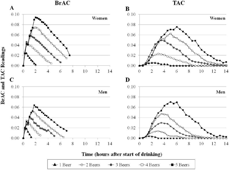
Time Course for actual mean BrAC (A and C) and actual mean TAC (B and D) achieved for women and men after drinking 1, 2, 3, 4, and 5 beers.
Also seen in Figure 1 is the fact that the time to peak for both BrAC and TAC vary as a function of the number of beers consumed which is partly due to the paced drinking procedure. There also was a time-lag between the measured TAC and BrAC levels which averaged 128.6 (SEM ± 5.4) minutes, but actually was an increasing linear function of the number of beers consumed (p < 0.001) and showed a non-significant trend for differences (p = 0.06) between men and women. This explains the importance of including “time-to-peak” as a factor in the models estimating peak BrAC from TAC data. Descriptive statistics for the actual peak TAC values observed as well as the actual and estimated peak BrAC are shown in Table 2 as a function of sex and beers consumed. From a total of 104 observations in the experiment, all peak BrAC values were greater than zero, but on the one beer day only, there were 8 observations (from 3 men and 5 women) out of 21, or 38%, in which peak TAC = 0. There were no observations in which peak TAC = 0 for the 2 through 5 beer consumption days.
Table 2. Means (M), standard deviations (SD), and ranges as a function of the number of beers consumed for peak TAC, peak BrAC, and estimated peak BrAC (Est. BrAC) for men and women.
| Number of Beers Consumed | ||||||
|---|---|---|---|---|---|---|
| 1 Beer | 2 Beers | 3 Beers | 4 Beers | 5 Beers | ||
|
| ||||||
| M ± SD (Range) | M ± SD (Range) | M ± SD (Range) | M ± SD (Range) | M ± SD (Range) | ||
| Men | Peak TAC | 0.005 ± 0.004 (0.000 - 0.010) | 0.015 ± 0.008 (0.007 - 0.036) | 0.034 ± 0.014 (0.011 - 0.056) | 0.052 ± 0.014 (0.029 - 0.072) | 0.075 ± 0.018 (0.044 - 0.103) |
| Peak BrAC | 0.023 ± 0.004 (0.011 - 0.028) | 0.036 ± 0.006 (0.024 - 0.045) | 0.045 ± 0.007 (0.034 - 0.053) | 0.054 ± 0.008 (0.042 - 0.069) | 0.067 ± 0.012 (0.051 - 0.088) | |
| Est. BrAC | 0.019 ± 0.012 (0.000 - 0.030) | 0.037 ± 0.005 (0.029 - 0.044) | 0.044 ± 0.006 (0.034 - 0.055) | 0.054 ± 0.007 (0.042 - 0.069) | 0.067 ± 0.009 (0.053 - 0.080) | |
|
| ||||||
| Women | Peak TAC | 0.006 ± 0.007 (0.000 - 0.020) | 0.026 ± 0.010 (0.012 - 0.046) | 0.053 ± 0.031 (0.015 - 0.102) | 0.069 ± 0.032 (0.034 - 0.121) | 0.084 ± 0.036 (0.046 - 0.152) |
| Peak BrAC | 0.029 ± 0.009 (0.016 - 0.044) | 0.049 ± 0.011 (0.038 - 0.072) | 0.065 ± 0.013 (0.050 - 0.088) | 0.079 ± 0.009 (0.067 - 0.094) | 0.098 ± 0.015 (0.080 - 0.120) | |
| Est. BrAC | 0.020 ± 0.021 (0.000 - 0.046) | 0.053 ± 0.007 (0.043 - 0.064) | 0.066 ± 0.014 (0.043 - 0.086) | 0.081 ± 0.015 (0.063 - 0.110) | 0.091 ± 0.016 (0.071 - 0.115) | |
Sample size was n=11 men and n=10 women except that n=10 men for the 5 Beer condition due to device failure.
Peak BrAC and Peak TAC levels achieved by men and women
As shown in Figure 2a, women had significantly higher peak BrAC levels (F(1, 19) = 34.12, p< 0.0001) compared to men. Post-hoc contrasts between men and women showed significant differences in peak BrAC levels after 2, 3, 4, and 5 beers (all p < 0.005). Sex-related differences in the slopes of peak BrAC levels were also observed (p < 0.001). In contrast to peak BrAC, there were no main sex differences observed in peak TAC levels (Figure 2b, F(1, 19) = 2.88, p= 0.11) or in the slopes of peak TAC levels as a function of beers consumed (p = 0.34).
Figure 2.

Linear regressions of (a) Peak BrAC levels in % BAC and (b) Peak TAC levels in g/dl shown by numbers of beers consumed in the five drinking conditions, plotting men (+, N = 54 observations) and women (O, N = 50 observations), separately.
Unaccounted sex differences in the relationship between BrAC and TAC
Correlations between peak BrAC and peak TAC levels for women and men are shown in Figure 3. While women had significantly higher peak BrAC levels than men (p< 0.0001), these elevations were not reflected in higher TAC readings. This discrepancy was observed as a significant sex-related difference in slope (p = 0.005), such that males had steeper slopes than females.
Figure 3.
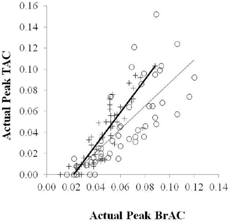
Associations between actual peak BrAC (% BAC) and peak TAC (g/dl) levels from current data, plotting men (+, N = 54 observations) and women (O, N = 50 observations) separately.
Developing a statistical model incorporating sex in the estimation of peak BrAC from TAC data
Data from all beers consumed were used in the model derivation -which included 96 observations with nonzero peak TAC values from the 21 participants. For those with zero peak TAC, the corresponding estimated peak BrAC was set at zero. We systematically considered adding the sex and sex-related variables (weight and BMI) alone and as 2- and 3-factor interactions to our original model estimating peak BrAC from the peak TAC and time-to-peak TAC variables. Sex, weight, and BMI were each considered separately and were statistically significant contributors in several models. However, these three variables were highly inter correlated (all p< 0.001), and so only one of these at a time were included in any particular model. Inclusion of sex in the model instead of weight or BMI achieved the best AIC values. Neither the addition of weight, BMI, or their substitution for the sex variable was superior to the simpler model including only sex. The optimal model selected for its simplicity and AIC optimization was determined to be the following equation (i.e., the fixed effect components of the final mixed-effects model): estimated peak BrAC = 0.02158 + 0.3940 *peak TAC + 0.000149 * time-to-peak TAC - 0.00366 * sex –0.1887 * peak TAC * sex.). Figure 4a shows that this equation resulted in a highly significant correlation between the estimated and the actual peak BrAC levels. This model significantly estimated peak BrAC with a high R2 of .76 (i.e., 76% of the variance in the peak BrAC). Post-Hoc correlations of estimated vs. actual peak BrAC for each level of beer drinking also showed highly significant correlations (all p<0.001) for drinking 2-5 beers, but not for 1 beer (p = 0.40) and there were no significant differences between the mean estimated and mean actual peak BrACs at any beer level (all p >0.20). Descriptive statistics for estimated peak BrAC are shown in Table 2. Finally, we further validated the model by showing that the estimated peak BrAC levels using this equation also correlated highly with the observed peak BrAC levels from the previous study (Dougherty et al. 2012), Spearman rs = 0.86, p< 0.0001 (Figure 4b).
Figure 4.
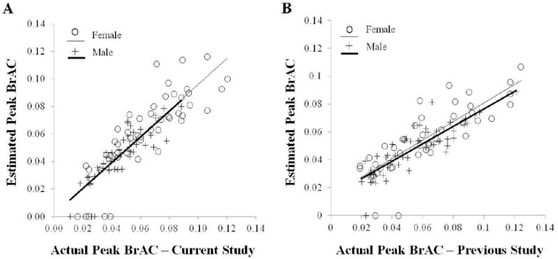
Scatterplot of association between actual peak BrAC (% BAC) and estimated peak BrAC (% BAC) using the model described herein for (a) the current study's data and (b) our previous study's data (Dougherty et al., 2012). Data are all values collected from all participants across all drinking conditions broken down as two regression slopes separately for men and women.
Discussion
The current study was designed to improve our previously reported (Dougherty et al., 2012) ability to use peak TAC readings to estimate peak BrAC levels by accounting for known and possible sex-related differences. This was achieved by having men and women both drink varying numbers of beers at the same rate to properly assess the effects of sex on the peak BrAC and TAC parameter readings. BrAC and TAC were measured concurrently to determine whether known sex-differences in blood alcohol would similarly affect TAC readings and/or affect peak BrAC predictions by our statistical model. We did observe that the actual peak BrAC levels were significantly higher in women compared to men, confirming previous observations of sex differences in the blood levels of alcohol attributable to differential absorption and distribution of alcohol in women (Baraona et al., 2001; Dettling et al., 2007; Jones and Jones, 1976). Comparable readings in TAC did not show significant sex differences but we did observe significant sex-dependent differences in the relationship between BrAC and TAC. We concluded that our statistical model to estimate peak BrAC levels from TAC data needed to include sex in the model to properly account for these effects. Using the actual TAC and BrAC data, and accounting for sex, we developed a statistical model that could account for 76% of the variance (R2) in peak BrAC. The optimal model included three variables: peak TAC, time-to-peak TAC, and sex. Lastly, to further validate the model, we applied it to an independent dataset collected in a previous study (Dougherty et al. 2012) and found that it accounted for similar amounts of variance.
It is worth noting that while positive TAC readings were recorded for all participants when two or more beers were consumed, that in a substantial percentage of cases (38%) no positive TAC readings were recorded after drinking only one beer (a higher percentage of women failed to achieve a positive TAC reading than men). This suggests that the transdermal alcohol monitoring may not be adequate in situations where the goal is to confirm abstinence. On the other hand, there is evidence that suggests that lower levels of drinking may be adequately discriminated from higher levels of drinking using transdermal alcohol monitoring. For example, we recently reported that a TAC cutoff of 0.024 g/dl could discriminate between participants who drank 1–2 drinks from those who consumed a larger number of drinks (Dougherty et al., 2012). Transdermal alcohol monitoring may be most appropriate in cases where research or clinical interventions focus on achieving moderation (rather than abstinence), which may be more consistent with more recent outcome goals (see Carey, Scott-Sheldon, Carey, & DeMartini, 2007).
We also confirmed previous findings that peak TAC readings show a time lag delay behind peak BrAC readings (Marques and McKnight 2007; 2009; Sakai et al, 2006; Swift, 2003). Marques and McKnight (2007; 2009), using a SCRAM monitor, reported an average of 4.5 hour time-lag between BrAC and TAC readings. They used an older model of the SCRAM device which had problems with water accumulation inside the unit over time which could dilute the alcohol, resulting in a delay in TAC readings. In the current study, the newest generation of the SCRAM device was used (SCRAM-II™) in which the company has reportedly fixed the water accumulation problem. Each participant wore a newly calibrated SCRAM-II device for the course of 5 days and the monitors were checked daily assuring that wear-related deterioration over time would not occur. Under the conditions of our study we observed an overall average of 129 minutes in time-lag between peak BrAC and peak TAC, but importantly, we also found that the time-lag was an increasing function of the number of beers. This finding may relate to Marques and McKnight's report that the rate elimination slope of TAC is more delayed than that of blood alcohol concentrations.
We also found that the relationship between peak TAC and peak BrAC differs in women compared to men; compared to actual peak BrAC, the peak TAC readings were relatively lower in women than in men. This finding confirms what was reported by Marques and McKnight (2007; 2009) who observed that women's peak TACs were 30.5% lower than their peak BrACs whereas men's peak TAC were 14.6% lower than their peak BrACs. This phenomenon was observed using two different transdermal alcohol monitoring devises including an older version of the SCRAM ankle monitor, and the Wrist Transdermal Alcohol Sensor (WrisTAS™) from Giner Inc. The reason for this lower peak TAC relative to peak BrAC in women is unknown, but may be related to sex differences in the skin. The skin of men and women differs anatomically, physiologically, and biochemically (reviewed in Giacomoni et al., 2009 and Tur, 1997). Though differences in skin thickness run counter to our findings, the skin of men is thicker than that of women in many areas of the body including calf-sites and forearms (Hattori and Okamoto, 1993; Sandby-Møller et al., 2003; Tur, 1997). Women also are known to have a significantly higher pH on their outermost layer of skin stratum corneum than men (Jacobi et al., 2005). Finally, women have a larger volume of subcutaneous fat compared to men in many areas of the body, including abdomen, calf and forearm (Cartier et al., 2009; Hattori et al., 1991; Liu et al., 2010; Westerbacka et al., 2004). As Marques and McKnight (2007, pg 47) indicate, “…it would be interesting to know whether skin pH or the higher subcutaneous adiposity of females accounts for flattening of the TAC peaks”. Taken together, the sex-related differences in peak BrAC to peak TAC ratios underscore the importance of accounting for sex in any model using TAC data to estimate peak BrAC levels.
The study has some limitations due to the controlled laboratory conditions under which participants were required to drink alcohol. More specifically, the specific amounts and rates of alcohol drinking may differ from real-world drinking behaviors. Clearly, variations in the rate of alcohol consumption may affect the TAC data variables used in the model for BrAC prediction (e.g., time-to-peak TAC and peak TAC). However, our findings of a high correlation between the actual BrAC and the model-corrected estimate of peak BrAC over a range of alcohol amounts (1-5 beers) suggest that these relationships are maintained during the course of a typical binge episode. Future studies should determine how alcohol drinking rate may affect these parameters in the prediction of BrAC levels and to extend these estimates and predictions to the outpatient environment where naturalistic drinking occurs. Preliminary data from our laboratory suggests that variations in rates of consumption do not affect the ability of our models to estimate peak BrAC.
In summary, the present findings indicate that it is important to account for sex in the model using TAC data to accurately estimate peak BrAC in both men and women. Peak breath alcohol or peak blood concentrations are used to describe maximum levels of intoxication which indeed are the most clinically relevant outcome relating to both health and safety guidelines. Clinical researchers, and perhaps practitioners, could benefit by using transdermal alcohol monitoring, which is a convenient, less burdensome, and continuous surrogate for more intrusive and less accurate measures (e.g., self-report and biological monitoring) of intoxication levels obtained only from peak BrAC readings. Our future work is focusing on developing methods to use these TAC data to estimate standardized units of alcohol consumed. The ability to better estimate both peak intoxication and number of drinks consumed will be important advancements in the field, which could have a significant impact on both research and clinical interventions for alcohol abuse and dependence.
Acknowledgments
Research reported in this publication was supported by the National Institute on Alcohol Abuse and Alcoholism of the National Institutes of Health [R01AA14988]. The research was also supported in part by the National Institute of Drug Abuse [T32DA031115] for postdoctoral training for Tara E. Karns. The content is solely the responsibility of the authors and does not necessarily represent the official views of the National Institutes of Health. Dr. Dougherty also gratefully acknowledges support from a research endowment, the William and Marguerite Wurzbach Distinguished Professorship. The authors appreciate the supportive functions performed by our valued colleagues Cameron Hunt and Krystal Shilling.
List of Abbreviations
- BMI
body mass index
- BrAC
breath alcohol concentration
- SCRAM
Secure Continuous Remote Alcohol Monitor
- TAC
transdermal alcohol concentration
Footnotes
None of the authors have conflicts of interests concerning this manuscript.
References
- Ahacic K, Kareholt I, Helgason AR, Allebeck P. Non-response bias and hazardous alcohol use in relation to previous alcohol-related hospitalization: comparing survey responses with population data. Subst Abuse Treat Prev Policy. 2013:8–10. doi: 10.1186/1747-597X-8-10. [DOI] [PMC free article] [PubMed] [Google Scholar]
- Akaike H. Information Theory and an Extension of the Maximum Likelihood Principle. In: Parzen E, Tanabe K, Kitagawa G, editors. Selected papers of Hirotugu Akaike. Springer; New York: 1998. pp. 199–213. [Google Scholar]
- Anderson JC, Hlastala MP. The kinetics of transdermal alcohol exchange. J Appl Physiol. 2006;100:649–655. doi: 10.1152/japplphysiol.00927. [DOI] [PubMed] [Google Scholar]
- Ayala J, Simons K, Kerrigan S. Quantitative determination of caffeine and alcohol in energy drinks and the potential to produce positive transdermal alcohol concentrations in human subjects. J Anal Toxicol. 2009;33:27–33. doi: 10.1093/jat/33.1.27. [DOI] [PubMed] [Google Scholar]
- Baraona E, Abittan CS, Dohmen K, et al. Gender differences in pharmacokinetics of alcohol. Alcohol Clin Exp Res. 2001;25:502–507. doi: 10.1111/j.1530-0277.2001.tb02242.x. [DOI] [PubMed] [Google Scholar]
- Barnett NP, Tidey J, Murphy JG, Swift R, Colby SM. Contingency management for alcohol use reduction: a pilot study using a transdermal alcohol sensor. Drug Alcohol Depend. 2011;118:391–399. doi: 10.1016/j.drugalcdep.2011.04.023. [DOI] [PMC free article] [PubMed] [Google Scholar]
- Bonomo YA, Bowes G, Coffey C, Carlin JB, Patton GC. Teenage drinking and the onset of alcohol dependence: a cohort study over seven years. Addiction. 2004;99:1520–1528. doi: 10.1111/j.1360-0443.2004.00846.x. [DOI] [PubMed] [Google Scholar]
- Bouchery EE, Harwood HJ, Sacks JJ, Simon CJ, Brewer RD. Economic costs of excessive alcohol consumption in the U.S., 2006. Am J Prev Med. 2011;41:516–524. doi: 10.1016/j.amepre.2011.06.045. [DOI] [PubMed] [Google Scholar]
- Breslin FC, Kapur BM, Sobell MB, Cappell H. Gender and alcohol dosing: a procedure for producing comparable breath alcohol curves for men and women. Alcohol Clin Exp Res. 1997;21:928–930. doi: 10.1111/j.1530-0277.1997.tb03860.x. [DOI] [PubMed] [Google Scholar]
- Carey KB, Scott-Sheldon LAJ, Carey MP, DeMartini KS. Individual-level interventions to reduce college student drinking: A meta-analytic review. Addictive Behaviors. 2007;32:2469–2494. doi: 10.1016/j.addbeh.2007.05.004. [DOI] [PMC free article] [PubMed] [Google Scholar]
- Cartier A, Côté M, Lemieux I, Pérusse L, Tremblay A, Bouchard C, Després JP. Sex differences in inflammatory markers: what is the contribution of visceral adiposity? Am J Clin Nutr. 2009;89:1307–1314. doi: 10.3945/ajcn.2008.27030. [DOI] [PubMed] [Google Scholar]
- CDC (Centers for Disease Control) [3 June 2013];Excessive Alcohol Use: Addressing a Leading Risk for Death, Chronic Disease, and injury: At a Glance 2011. 2011 http://www.cdc.gov/chronicdisease/resources/publications/aag/alcohol.htm.
- CDC (Centers for Disease Control) [April 29, 2013];Fact Sheets- Alcohol Use and Health. 2012 at http://www.cdc.gov/alcohol/fact-sheets/alcohol-use.htm.
- Dawson DA, Grant BF, Li TK. Quantifying the risks associated with exceeding recommended drinking limits. Alcohol Clin Exp Res. 2005;29:902–908. doi: 10.1097/01.ALC.0000164544.45746.A7. [DOI] [PubMed] [Google Scholar]
- de Visser RO, Birch JD. My cup runneth over: young people's lack of knowledge of low-risk drinking guidelines. Drug Alcohol Rev. 2012;31:206–212. doi: 10.1111/j.1465-3362.2011.00371.x. [DOI] [PubMed] [Google Scholar]
- Del Boca FK, Darkes J. The validity of self-reports of alcohol consumption: state of the science and challenges for research. Addiction. 2003;98:1–12. doi: 10.1046/j.1359-6357.2003.00586.x. [DOI] [PubMed] [Google Scholar]
- Dettling A, Fischer F, Bohler S, et al. Ethanol elimination rates in men and women in consideration of the calculated liver weight. Alcohol. 2007;41:415–420. doi: 10.1016/j.alcohol.2007.05.003. [DOI] [PubMed] [Google Scholar]
- Devos-Comby L, Lange JE. Standardized measures of alcohol-related problems: a review of their use among college students. Psychol Addict Behav. 2008;22:349–361. doi: 10.1037/0893-164X.22.3.349. [DOI] [PubMed] [Google Scholar]
- Department of Health and Human Services: Substance Abuse and Mental Health Services Administration. [3 June 2013];Results from the 2001 National Household Survey on Drug Abuse: Summary of National Findings. 2002 I http://www.samhsa.gov/data/nhsda/2k1nhsda/pdf/cover.pdf. [Google Scholar]
- Dougherty DM, Charles NE, Acheson A, John S, Furr RM, Hill-Kapturczak N. Comparing the detection of transdermal and breath alcohol concentrations during periods of alcohol consumption ranging from moderate drinking to binge drinking. Exp Clin Psychopharmacol. 2012;20:373–381. doi: 10.1037/a0029021. [DOI] [PMC free article] [PubMed] [Google Scholar]
- First MB, Spitzer RL, Givvon M, Williams JBW. Structured Clinical Interview for DSM-IV-TR Axis I Disorders, Research Version, Non-patient Edition (SCID-I/NP) New York: Biometrics Research, New York State Psychiatric Institute; 2001. [Google Scholar]
- Giacomoni PU, Mammone T, Teri M. Gender-linked differences in human skin. J Dermatol Sci. 2009;55:144–149. doi: 10.1016/j.jdermsci.2009.06.001. [DOI] [PubMed] [Google Scholar]
- Hahn JA, Woolf-King SE, Muyindike W. Adding fuel to the fire: alcohol's effect on the HIV epidemic in Sub-Saharan Africa. Curr HIV/AIDS Rep. 2011;8:172–180. doi: 10.1007/s11904-011-0088-2. [DOI] [PubMed] [Google Scholar]
- Hattori K, Numata N, Ikoma M, Matsuzaka A, Danielson RR. Sex differences in the distribution of subcutaneous and internal fat. Hum Biol. 1991;63:53–63. Retrieved from http://www.jstor.org/stable/41464142?origin=JSTOR-pdf. [PubMed] [Google Scholar]
- Hattori K, Okamoto W. Skinfold compressibility in Japanese university students. Okajimas Folia Anat Jpn. 1993;70:69–77. doi: 10.2535/ofaj1936.70.2-3_69. [DOI] [PubMed] [Google Scholar]
- Helander A, Peter O, Zheng Y. Monitoring of the alcohol biomarkers PEth, CDT and EtG/EtS in an outpatient treatment setting. Alcohol Alcohol. 2012;47:552–557. doi: 10.1093/alcalc/ags065. [DOI] [PubMed] [Google Scholar]
- Jacobi U, Gautier J, Sterry W, Lademann J. Gender-related differences in the physiology of the stratum corneum. Dermatology. 2005;211:312–317. doi: 10.1159/000088499. [DOI] [PubMed] [Google Scholar]
- Javors MA, Johnson BA. Current status of carbohydrate deficient transferrin, total serum sialic acid, sialic acid index of apolipoprotein J and serum beta-hexosaminidase as markers for alcohol consumption. Addiction. 2003;98:45–50. doi: 10.1046/j.1359-6357.2003.00582.x. [DOI] [PubMed] [Google Scholar]
- Jones BM, Jones MK. Alcohol effects in women during the menstrual cycle. Ann N Y Acad Sci. 1976;273:576–587. doi: 10.1111/j.1749-6632.1976.tb52931.x. [DOI] [PubMed] [Google Scholar]
- Kerr WC, Stockwell T. Understanding standard drinks and drinking guidelines. Drug Alcohol Rev. 2012;31:200–205. doi: 10.1111/j.1465-3362.2011.00374.x. [DOI] [PMC free article] [PubMed] [Google Scholar]
- Leffingwell TR, Cooney NJ, Murphy JG, et al. Continuous objective monitoring of alcohol use: twenty-first century measurement using transdermal sensors. Alcohol Clin Exp Res. 2013;37:16–22. doi: 10.1111/j.1530-0277.2012.01869.x. [DOI] [PMC free article] [PubMed] [Google Scholar]
- Liu J, Fox CS, Hickson DA, May WD, Hairston KG, Carr JJ, Taylor HA. Impact of abdominal visceral and subcutaneous adipose tissue on cardiometabolic risk factors: the Jackson Heart Study. J Clin Endocrinol Metab. 2010;95:5419–5426. doi: 10.1210/jc.2010-1378. [DOI] [PMC free article] [PubMed] [Google Scholar]
- Marques PR. Levels and types of alcohol biomarkers in DUI and clinic samples for estimating workplace alcohol problems. Drug Test Anal. 2012;4:76–82. doi: 10.1002/dta.384. [DOI] [PMC free article] [PubMed] [Google Scholar]
- Marques PR, McKnight AS. National Highway Traffic Safety Administration. Evaluating transdermal alcohol measuring devices (Report No DOT HS 810 875) Washington, DC: U.S Government; 2007. [Google Scholar]
- Marques PR, McKnight AS. Field and laboratory alcohol detection with 2 types of transdermal devices. Alcohol Clin Exp Res. 2009;33:703–711. doi: 10.1111/j.1530-0277.2008.00887.x. [DOI] [PubMed] [Google Scholar]
- Marques P, Tippetts S, Allen J, et al. Estimating driver risk using alcohol biomarkers, interlock blood alcohol concentration tests and psychometric assessments: initial descriptives. Addiction. 2010;105:226–239. doi: 10.1111/j.1360-0443.2009.02738.x. [DOI] [PMC free article] [PubMed] [Google Scholar]
- Mokdad AH, Marks JS, Stroup DF, Gerberding JL. Actual causes of death in the United States, 2000. J Amer Med Assoc. 2004;291:1238–1245. doi: 10.1001/jama.291.10.1238. [DOI] [PubMed] [Google Scholar]
- Nakagawa S, Schielzeth H. A general and simple method for obtaining R2 from generalized linear mixed-effects models. Methods in Eco and Evol. 2013;4:133–142. doi: 10.1111/j.2041-210x.2012.00261.x. [DOI] [Google Scholar]
- National Institute of Alcohol Abuse and Alcoholism (NIAAA) [3 June 2013];National Institute of Alcohol Abuse and Alcoholism Council Approves Definition of Binge Drinking. NIAAA Newsletter, No 3. 2004 http://pubs.niaaa.nih.gov/publications/newsletter/winter2004/newsletter_number3.pdf.
- National Institute of Alcohol Abuse and Alcoholism (NIAAA) [May 1, 2013];Moderate and Binge Drinking. 2014 at http://www.niaaa.nih.gov/alcohol-health/overview-alcohol-consumption/moderate-binge-drinking.
- Rehm J, Gmel G, Sempos CT, Trevisan M. Alcohol-related morbidity and mortality. Alcohol Res Health. 2003a;27:39–51. [PMC free article] [PubMed] [Google Scholar]
- Rehm J, Room R, Graham K, Monteiro M, Gmel G, Sempos CT. The relationship of average volume of alcohol consumption and patterns of drinking to burden of disease: an overview. Addiction. 2003b;98:1209–1228. doi: 10.1046/j.1360-0443.2003.00467.x. [DOI] [PubMed] [Google Scholar]
- Robin RW, Long JC, Rasmussen JK, Albaugh B, Goldman D. Relationship of binge drinking to alcohol dependence, other psychiatric disorders, and behavioral problems in an American Indian tribe. Alcohol Clin Exp Res. 1998;22:518–523. doi: 10.1111/j.1530-0277.1998.tb03682.x. [DOI] [PubMed] [Google Scholar]
- Sakai JT, Mikulich-Gilbertson SK, Long RJ, Crowley TJ. Validity of transdermal alcohol monitoring: fixed and self-regulated dosing. Alcohol Clin Exp Res. 2006;30:26–33. doi: 10.1111/j.1530-0277.2006.00004.x. [DOI] [PubMed] [Google Scholar]
- Sandby-Møller J, Poulsen T, Wulf HC. Epidermal thickness at different body sites: Relationship to age, gender, pigmentation, blood content, skin type and smoking habits. Acta Derm Venereol. 2003;83:410–413. doi: 10.1080/00015550310015419. [DOI] [PubMed] [Google Scholar]
- Schulenberg J, O'Malley PM, Bachman JG, Wadsworth KN, Johnston LD. Getting drunk and growing up: trajectories of frequent binge drinking during the transition to young adulthood. J Stud Alcohol. 1996;57:289–304. doi: 10.15288/jsa.1996.57.289. [DOI] [PubMed] [Google Scholar]
- Schulenberg JE, Maggs JL. A developmental perspective on alcohol use and heavy drinking during adolescence and the transition to young adulthood. J Stud Alcohol Suppl. 2002;14:54–70. doi: 10.15288/jsas.2002.s14.54. [DOI] [PubMed] [Google Scholar]
- Sobell LC, Sobell MB. Alcohol Consumption Measures. Assessing Alcohol Problems: Guide for Clinicians and Researchers. (2) 2003:77–99. [Google Scholar]
- Swift R. Transdermal alcohol measurement for estimation of blood alcohol concentration. Alcohol Clin Exp Res. 2000;24:422–423. doi: 10.1111/j.1530-0277.2000.tb02006.x. [DOI] [PubMed] [Google Scholar]
- Swift R. Direct measurement of alcohol and its metabolites. Addiction. 2003;98:73–80. doi: 10.1046/j.1359-6357.2003.00605.x. [DOI] [PubMed] [Google Scholar]
- Swift RM, Martin CS, Swette L, LaConti A, Kackley N. Studies on a wearable, electronic, transdermal alcohol sensor. Alcohol Clin Exp Res. 1992;16:721–725. doi: 10.1111/j.1530-0277.1992.tb00668.x. [DOI] [PubMed] [Google Scholar]
- Tur E. Pysiology of the skin—differences between women and men. Clin Dermatol. 1997;15:5–16. doi: 10.1016/S0738-081X(96)00105-8. [DOI] [PubMed] [Google Scholar]
- Wechsler H, Nelson TF. Binge drinking and the American college student: what's five drinks? Psychol Addict Behav. 2001;15:287–291. doi: 10.1037/0893-164X.15.4.287. [DOI] [PubMed] [Google Scholar]
- Westerbacka J, Cornér A, Tiikkainen M, Tamminen M, Vehkavaara S, Häkkinen AM, Fredriksson J, Yki-Järvinen H. Women and men have similar amounts of liver and intra-abdominal fat, despite more subcutaneous fat in women: implications for sex differences in markers of cardiovascular risk. Diabetologia. 2004;47:1360–1389. doi: 10.1007/s00125-004-1460-1. [DOI] [PubMed] [Google Scholar]
- White AM, Kraus CL, McCracken LA, Swartzwelder HS. Do college students drink more than they think? Use of a free-pour paradigm to determine how college students define standard drinks. Alcohol Clin Exp Res. 2003;27:1750–1756. doi: 10.1097/01.ALC.0000095866.17973.AF. [DOI] [PubMed] [Google Scholar]