Efficient Discovery of De-identification Policies Through a Risk-Utility Frontier

Abstract

Modern information technologies enable organizations to capture large quantities of person-specific data while providing routine services. Many organizations hope, or are legally required, to share such data for secondary purposes (e.g., validation of research findings) in a de-identified manner. In previous work, it was shown de-identification policy alternatives could be modeled on a lattice, which could be searched for policies that met a prespecified risk threshold (e.g., likelihood of re-identification). However, the search was limited in several ways. First, its definition of utility was syntactic - based on the level of the lattice - and not semantic - based on the actual changes induced in the resulting data. Second, the threshold may not be known in advance.

The goal of this work is to build the optimal set of policies that trade-off between privacy risk (R) and utility (U), which we refer to as a R-U frontier. To model this problem, we introduce a semantic definition of utility, based on information theory, that is compatible with the lattice representation of policies. To solve the problem, we initially build a set of policies that define a frontier. We then use a probability-guided heuristic to search the lattice for policies likely to update the frontier. To demonstrate the effectiveness of our approach, we perform an empirical analysis with the Adult dataset of the UCI Machine Learning Repository. We show that our approach can construct a frontier closer to optimal than competitive approaches by searching a smaller number of policies. In addition, we show that a frequently followed de-identification policy (i.e., the Safe Harbor standard of the HIPAA Privacy Rule) is suboptimal in comparison to the frontier discovered by our approach.

1. Introduction

In the age of big data, organizations from a wide range of domains (e.g., finance, healthcare, homeland security, and social media) will accumulate a substantial quantity of detailed personal data [7, 25]. These large-scale resources will support the development of novel applications and refinement of innovative services. For instance, healthcare facilities are increasingly adopting electronic medical record systems and high-throughput genotyping technologies, which, in turn, have enabled the discovery of personalized treatment regimens [34]. At the same time, there are many pressures to publish person-level data to support information reuse and transparency (e.g., [3, 18, 46]) and adhere to federal requirements (e.g., [29]). While publication enables broad access, there are also concerns that it can violate personal privacy rights [5, 17, 31].

To mitigate privacy threats, various laws and regulations recommend that personal data be de-identified before dissemination (e.g., the EU Data Protection Directive [1] and the US Health Insurance Portability and Accountability Act (HIPAA) [45]). The concept of de-identification is somewhat subjective [35], but is often tied to the notion of re-identification (oftentimes referred to as identity disclosure [21]) risk. While we recognize there are concerns that de-identified data may be re-identified [30], it remains a core principle of privacy regulation [41]. Technically, an organization may adopt various approaches to accomplish de-identification. In this research, we focus on the application of generalization, a common strategy in de-identification policies [12]. The application of such policies has a direct influence on the usability of the resulting data [32]. As a consequence, it is critical that the policy selected for de-identification appropriately balance the competing needs of minimizing risk (R) and maximizing utility (U).

As we recount in the following section, there have been several attempts to achieve this balance. The majority have focused on optimization in the context of anonymization (e.g., k-anonymity [4]), but this is a more rigid formalism than de-identification [28]. Anonymization provides guarantees of protection for each record in a dataset, but de-identification is often a rules-driven policy (e.g., “recode all ages over 90 as 90+”). As such, previous optimization approaches are not as flexible in their policy definitions. To the best of our knowledge, the only work that provides a data structure for such an optimization is the work in [6]. However, their work is limited in several crucial ways. First, it models data utility from a syntactic perspective (e.g., “How many ages are generalized?”) as opposed to a semantic perspective (e.g., “How does the generalization of age influence the distribution of patients?”). Second, it does not allow for a complete analysis of the tradeoff between privacy and utility. Rather, it assumes that a privacy risk threshold is known (or can be computed) a priori, whereupon it then searches for alternative strategies with risk no greater than the threshold.

As we show in this work, the framework of [6] can be extended to overcome this limitation. To do so, we introduce a semantic utility function and model the de-identification policy search problem as a dual-objective optimization. Thus, our goal is to detect a set of policies that form an R-U frontier, which offers a collection of mutually exclusive de-identification policies. The visualization of such a frontier should provide intuition into the tradeoff between utility and risk for policy alternatives. While the space of possible policies is too large to perform a systematic exhaustive in practical time, we introduce an efficient strategy to navigate the policy space and construct an approximation of the frontier. More specifically, our work has three primary contributions:

• Problem formalization: We provide a rigorous definition of the de-identification policy frontier discovery (DPFD) problem. We show how this problem relates to a lattice of policies and measures for re-identification risk and data utility.

• Search Strategies: Based on the policy lattice, we develop a novel search strategy, guided by probability-based heuristics, that can construct an approximate frontier efficiently.

• Empirical Evaluation: We perform an empirical study on the Adult dataset and demonstrate that our approach is more effective than a competitive search strategy, in terms of the frontier discovered and time required to do so. Moreover, we illustrate how a common health data de-identification policy (i.e., HIPAA Safe Harbor) is suboptimal to the frontier discovered by our policy.

The remainder of this paper is organized as follows. In Section 2, we review related work in optimization strategies for data privacy, with a particular focus on anonymization and statistical disclosure control frameworks. In Section 3, we formalize the DPFD problem and several algorithms for solving the problem. In Section 4, we present an empirical evaluation of our search strategy. In Section 5, we discuss the contributions and limitations of this work and in Section 6 we offer several conclusions.

2. Related Work

In this section, we review frameworks and strategies for optimizing the search for anonymization and de-identification solutions. This topic is a portion of the broader issue of privacy-preserving data publishing, for which we direct readers to [15] for an excellent survey.

2.1 Search for Anonymization Solutions

Many variations of formal anonymization have been proposed, but the literature primarily focuses on optimization for the k-anonymity protection model [40]. In effect, k-anonymization is a special case of de-identification and thus illustrates the complexity of our problem. k-anonymization dictates that each published record must be equivalent to k–1 other published records. This technique is often applied to a quasi-identifier (QI), which is the set of attributes (e.g., date of birth and residential ZIP code) that link a record to a resource containing explicit identifiers (e.g., personal name) [9]. QI attributes have traditionally been formalized as domain generalization hierarchies (DGHs) that can be systematically enumerated [39]. However, the search for the k-anonymous solution which minimizes the total quantity of generalization is an NP-hard problem [2, 27], which has led to a large and growing collection of search strategies [8]. Here, we review the most relevant to our work.

[39] introduced the concept of full-domain generalization in which all values of each attribute are generalized to the same level of the DGH. This paper also proposed greedy heuristics to generate k-anonymous solutions. [33] showed the generalization space maps to a partially ordered lattice and introduced a binary search method, which guarantees the solution is optimal according to a certain cost metric.

By relaxing the constraint of mapping the entire domain to the same level of the DGH, [19] defined the generalization solution space as all arbitrary partitions on the ordered set of values in a single attribute's domain (e.g., age 14 is reported as 10-15 while age 16 is reported as 16-30). Given that the size of the search space is exponential in the size of a QI's domain, exhaustive search strategies are impractical. Thus, [19] proposed a genetic algorithm, to perform a partial search of the generalization space. This work is also notable because it represents QIs and their generalization as bit-strings, a model we adopt in this paper. Since genetic algorithms do not provide a guarantee about the optimality of the solution and are often associated with long runtimes, [16] restructured the space of [19] to a tree and provided a systematic search algorithm using pruning and rearrangement to find an optimal k-anonymization in a practical amount of time. [23] further expanded the solution space to permit arbitrary partitioning of each attribute domain without forcing a total order on it. Based on this partitioning, they proposed a novel method to create a partition enumeration tree and search algorithms to efficiently discover the optimal anonymization solution.

In all the generalization strategies mentioned above, each attribute is generalized independently (i.e., a single-dimension attribute domain). Thus any specific value in each domain is generalized in the same way in every tuple of the dataset. [22] extended this model to a multi-dimensional space by generalizing values of tuples in the dataset. A greedy partitioning strategy was introduced to discover a k-anonymization solution. While flexible (e.g., females with age 14 are expressed as [female, 14] while males with age 14 are expressed as [male, 10-14]), the expansion of the search space provides more generalization options. As a result, the anonymized dataset can be confusing for users because the same value of a QI attribute can be mapped to different values in the same anonymized dataset.

2.2 Search for De-identification Solutions

As mentioned earlier, the work most closely related to ours is that of [6]. The space of possible solutions is modeled as the lattice introduced in [19]. However, the privacy goal is not k-anonymization. Instead, risk is modeled as the expected number of records likely to be re-identified under a certain policy (e.g., HIPAA Safe Harbor).

The lattice is searched for policies that have risk no worse than the prespecified policy. The search process is accomplished through a bisecting search. Our work generalizes and extends this framework. A fundamental difference is that [6] searches for policies with minimum cost that satisfy the predefined risk, whereas in this paper the search is a dual-objective optimization problem.

2.3 Frontiers and Data Privacy

The idea of frontier optimization for privacy protection derives from the Risk-Utility (or R-U) confidentiality map [11] which was first used to assess different statistical disclosure control (SDC) methods based on the optimal tradeoff between risk and utility. [37] introduced a framework that maps SDC methods to an R-U confidentiality map to determine optimal parameterizations for such techniques. Based on this framework, [36] performed an empirical analysis of SDC methods for standard tabular outputs(e.g., swapping, rounding). [42] also adopted the R-U confidentiality map as an optimal criterion for data release. Given its roots in the statistical domain, the R-U confidentiality map was initially applied to protection strategies based on perturbation (e.g., randomization), as opposed to the generalization techniques more commonly found in de-identification.

In the context of data anonymization, the R-U confidentiality map is composed of a set of scattering points mapped from a generalization space instead of a simple curve in previous SDC applications. To explicitly represent the optimal solution curve in the R-U space, the concept of frontier is introduced to the R-U confidentiality framework [24]. It was demonstrated that k-anonymization can be framed as a dual-objective optimization in the R-U space. [24] uses the algorithm in [22] to discover anonymization solutions to map to the R-U space. [26] adopted R-U confidentiality map to transaction data anonymization. [10] also framed k-anonymization as a dual-objective optimization problem. In their framework, the solution space is the lattice structure introduced by [19], which is searched using a genetic algorithm. This approach, however, has several limitations in comparison to the strategy we offer in this paper. In particular, the genetic algorithm is slow and is not clearly guided by the semantics (e.g., risk and utility) of its solutions. By contrast, our algorithm is a combination of systematic and stochastic search and uses several monotonicity cost properties on the lattice to prune large sections from consideration.

3. Methods

In this section, we present the de-identification policy frontier discovery (DPFD) problem. First, we define a policy search space, a mapping of the policy space to the R-U space, and the formalization of the search problem. Second, we introduce several search algorithms to systematically explore the policy space.

3.1 De-identification Policy

We assume the data to be published is organized in a table for which the explicit identifying attributes (e.g., personal name and Social Security number) have already been suppressed. The remaining attributes of the table constitute the QI and each tuple corresponds to a distinct individual. To de-identify the data, the specific QI values will either i) remain in their specific state or ii) be recoded with more general, but semantically consistent, values.

Different generalization models induce different de-identification polices. In this work, we require a total order in the domain of each QI attribute and apply a full-subtree generalization model [22], which means that the values in a domain are mapped to a set of non-overlapping intervals. As such, a mapping function can be defined by the corresponding partition on the domain of a QI attribute.

Formally, a de-identification policy corresponds to the set of domain partitions (Definition 3.1) for each QI attribute (Definition 3.2).

Definition 3.1 (Domain Partition). Let D be a totally ordered domain and p be a set of intervals on D: p = { I₁, …, I_l}, where l is the number of intervals. p is a partition on D if ∀i ≠ j, I_i ∩ I_j = Ø and ${\cup }_i^l{I}_i=D$.

Definition 3.2 (de-identification policy). Let Q = {Q₁, …, Q_n} be a set of quasi-identifying attributes. Let us assume D_i is the domain of Q_i and p_i is a partition on D_i. The set {p₁, …, p_n} is a de-identification policy.

Figure 1 provides an example of a de-identification policy. The set of QI attributes is {Age, Gender, ZIP} and the domains are {1, …, 10}, {male, female}, and {37201, …, 37229}, respectively. In this policy Age, Gender, and ZIP are mapped to the aggregated groups: [1-2], [3-6] and [7-10]; [female] and [male]; and [37201, …, 37228] and [37229], respectively. This policy is valid because the aggregated groups of values for each QI compose a partition of the corresponding domain. By contrast, a mapping of ages to [1 – 5] and [3 – 10] does not constitute a valid policy because the intervals overlap (i.e., 3, 4, or 5 could be in either interval).

Figure 1. An example of a de-identification policy defined over three quasi-identifying attributes, {Age, Gender, ZIP}.

We use the full subtree generalization model because it offers several advantages over alternative models. First, as shown in [6], it enables representation of fine-grained policies, as well as common policies encountered in the real world (e.g., HIPAA Safe Harbor). Second, the set of policies can be structured as a lattice of generalizations which can be systematically searched. Third, it is straightforward to interpret how a policy changes the syntax of the data.

3.2 Policy Space Formalization

3.2.1 Policy Representation

In our model, policies are modeled as bit-strings. To characterize the translation, let n be the number of values in the domain of a QI attribute. After enforcing a total order on the values, they are mapped to a bit-string of size n – 1. The original domain is represented by a bit-string of 1's, whereas a bit of 0 indicates a demarcation in the partition has been removed to widen an interval¹ (i.e., values have been generalized). For example, the bit-string for Age in Figure 1 is [0, 1, 0, 0, 0, 1, 0, 0, 0].

A de-identification policy α is the concatenation of the bit-string for each QI attribute. In the remainder of this paper, we use the term de-identification policy to refer to both the actual policy and its bit-string representation when the meaning is unambiguous. For reference, we use α[i] to represent the value of the i^th bit.

3.2.2 Partial Order of Policies

The policy space contains all possible bit-string permutations, which are partially ordered. We use ≺ to refer to the ordering on two policies as follows:

Definition 3.3 (≺). Given policies α and β, we say α ≺ β if

$$\forall i\left(\alpha \left[i\right]=1\to \beta \left[i\right]=1\right)\wedge \exists i\left(\alpha \left[i\right]=0\wedge \beta \left[i\right]=1\right)$$

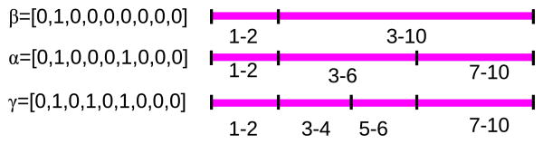
By this definition, α is more general than β because we can derive β by making smaller intervals in the partition (i.e., flipping bits from 0 to 1). As an example, Figure 2 depicts three policies for Age. It can be seen that α is the same policy as γ without the demarcation between ages 4 and 5. Similarly, β removes the demarcation between ages 6 and 7. As such, β ≺ α ≺ γ and the de-identified data derived from 7 will be at least as specific as the data derived from α.

Figure 2. An example of GLB. β is a GLB of α, while a is α GLB of γ.

We define the Greatest Lower Bound (GLB) over the policy space as follows:

Definition 3.4 (Greatest Lower Bound (GLB)). Policy α is a GLB of policy β, if

$$\exists i\left(\alpha \left[i\right]=0\wedge \beta \left[i\right]=1\wedge \forall j\left(j\ne i\to \beta \left[j\right]=\alpha \left[j\right]\right)\right).$$

In Figure 2, β is a GLB of α while a is a GLB of γ.

The most general policy (i.e., all 0's) and the most specific policy (i.e., all 1's), are referred to as top and bottom, respectively.

3.2.3 Policy Lattice

Based on the partial ordering, the policy space can be structured in a lattice. An example of such a lattice is depicted in Figure 3. The nodes in this lattice are composed of all bit-strings of length n. There is a directed edge from policy α to policy β, if, and only if, α is a GLB of β.

Figure 3.

An example of a de-identification policy lattice with five quasi-identifying values. Rectangular nodes depict a maximal chain, while oval nodes represent a sublattice.

In preparation for our policy search algorithms, we define two types of subgraphs over the lattice: 1) chain and 2) sub-lattice. A chain (Definition 3.5) is a totally ordered subset in the lattice. A maximal chain is one that is not a proper subset of any other chain.

Definition 3.5 (Chain). A sequence of policies C: α₁ ≺ α₂ ≺ ⋯ ≺ α_n is a chain if, and only if ∀i, α_i is a GLB of α_i+1. The chain is a maximal chain if and only if, α₁ is top and α_n is bottom.

In Figure 3, the rectangular nodes (i.e., [0, 0, 0, 0], [1, 0, 0, 0], [1, 1, 0, 0], [1, 1, 1, 0], [1, 1, 1, 1]) constitute a maximal chain.

A sublattice (Definition 3.6) is a subgraph i) bounded by an upper node and lower node on some chain and ii) contains every node in the set of all chains between them. Any two policies with a chain between them can define a sublattice.

Definition 3.6 (Sublattice). Given policies α and β, if α ≺ β, then the set {p∣α ≺ p ∧ p ≺ β} is a sublattice. This set is referred to as sublattice (α, β), where α and β are the upper and lower policies of the sublattice, respectively.

An example of a sublattice is shown in the oval nodes of Figure 3. Here sublattice([0, 0, 0, 1], [1, 0, 1, 1]) defines the set {[0, 0, 0, 1], [0, 0, 1, 1], [1, 0, 0, 1], [1, 0, 1, 1]}.

3.3 Policy Frontier Search Problem

3.3.1 Risk and Utility Measurement

To map a policy to the R-U space, we assess its risk and utility with respect to the data under consideration for dissemination. To enable an efficient search, it is crucial to ensure the order of risk and utility scores are consistent with the natural partial order in the policy space. This notion is formalized through the following order homomorphisms:

Definition 3.7 (Risk Order Homomorphism). Given a policy lattice S and a data table T, a risk function R_T(α) satisfies a risk order homomorphism if ∀α, β ∈ S, α ≺ β → R_T (α) ≤ R_T (β).

Definition 3.8 (Utility Order Homomorphism). Given policy lattice S and a data table T, an information loss function U_T (α) satisfies a utility order homomorphism if ∀α, β ∈ S, α ≺ β → U_T(α) ≥ U_T(β),

3.4 Policy Frontier

By applying risk and utility functions that satisfy their respective homomorphisms, each policy in the lattice is mapped into the R-U space to be searched for frontier policies.

To define a frontier, we introduce the notion of a strictly dominated relationship:

Definition 3.9 (Strictly Dominated). Given policies α and β and a data table T, α is strictly dominated by β if

$$\left(R_T\left(\beta \right)\le R_T\left(\alpha \right)\right)\wedge \left(U_T\left(\beta \right)\le U_T\left(\alpha \right)\right)$$

and

$$\left(R_T\left(\beta \right)<R_T\left(\alpha \right)\right)\vee \left(U_T\left(\beta \right)<U_T\left(\alpha \right)\right).$$

Informally, policy β strictly dominates policy α if both risk and utility values of β are no greater than the corresponding values of α and at least one value of β is strictly less that of α. The dominated relationship defines a partial order in the R-U space. Based on this partial order, the frontier corresponds to the set of policies for which we have found no dominating policies:

Definition 3.10 (Frontier). Given a policy lattice S, the frontier is the non-dominated set of policies {α∣α ∈ S ∧ ∄β (β ∈ S ∧ β strictly dominates α)}.

The goal of the de-identification policy frontier discovery (DPFD) problem is to find all frontier policies in a lattice.

3.5 Search Algorithms

The size of a typical policy lattice is too large for an exhaustive, systematic search. Thus, we developed two heuristic approaches: 1) Random Chain Search and 2) Heuristic Sublattice Search.

3.5.1 Random Chain

The first strategy is called the Random Chain Search (RCS) and is shown in Algorithm 1.

The process begins by assigning an arbitrary non-dominated set of policies in the lattice to the frontier, which is accomplished through InitializeFrontier()². Next, we itera-tively select maximal random chains, via the selectRandom-Chain(), and update the frontier with policies on the chains. This process iterates until n policies have been searched. Updating the frontier is accomplished through the function updateFrontier(f, α), which attempts to revise the frontier f with each policy α in the chain. If the frontier does not contain policies that dominate α, it is inserted into the frontier. The frontier then drops all policies dominated by α. As an example of this function, consider Figure 4(a).

Figure 4.

An example of updating the frontier in the R-U space using policies from Figure 3. The current frontier is composed of policies mapped to the stair-step curve. In 4(a), the policy mapped to the square will be added to the frontier because it dominates policies currently on the frontier (i.e., [1, 1, 0, 0] and [1, 1, 1, 0]), which will be removed. In 4(b), the rectangle represents the bounding region of the R-U mapping of policies in sublattice ([0, 0, 0, 1], [1, 0, 1, 1])

Algorithm 1 Random Chain Search (RCS)
Input: n, the maximum number of policies to estimate; L, the length of a policy; T, a dataset
Output: f, the frontier policies
1:	i ← 0
2:	f ← InitializeFrontier() {This function returns a non-dominated set of policies, including top and bottom.}
3:	while i < n do
4:	c ← selectRandomChain() {This function begins at bottom. It iteratively selects a policy at random from the GLB, to which it proceeds until it reaches top. It returns all the policies selected.}
5:	for all α in c do
6:	f ← updateFrontier (f,α)
7:	end for
8:	i ← i + L {L is the number of policies on the chain}
9:	end while
10:	return f

3.5.2 Sublattice Heuristic Search

The RCS algorithm is naïve in that it assumes all regions of the lattice are equally likely to update the frontier. However, this is not the case, and we suspect sublattices can be compared to the frontier to search more efficiently. Consider, given a frontier f, we can draw a stair-step curve in the R-U space that connects all policies on the frontier. An example of such a curve is depicted in Figures 4(a) and 4(b). It is clear that any policy mapped to the region above the curve will be dominated by at least one policy on the frontier. Additionally, any policy mapped to the region below the frontier will always update the frontier. Thus, this curve divides the R-U space into two regions: 1) dominated and 2) non-dominated.

Given sublattice(α, β), it can be proven that the risk and utility values of policies in the sublattice are bounded in a rectangle defined by the risk and utility values of policies α and β, which we call the bounding region. In other words, all policies in the sublattice will have risk in the range [R_T(α), R_T(β)] and utility in the range [U_T(β), U_T(α)].³ For example, in Figure 3, all policies in sublattice([0, 0, 0, 1], [1, 0, 1, 1]) are mapped to the rectangular area bounded by the R-U mapping of the top and bottom policies of the frontier in Figure 4(b).

To leverage this fact from a probabilistic perspective, we assume that the policies in a sublattice are uniformly distributed in the bounding rectangle. This implies the probability that a policy in a sublattice updates the frontier is the proportion of the lattice's bounding rectangle which falls below the curve of the frontier. Formally, imagine policies on the frontier f are mapped to a set of R-U points that are ordered increasingly by risk {(r₀, u₀), …, (r_h, u_h)}, where h is the number of polices on the frontier. Now, given sublattice(α, β), let us assume the policies α and β are mapped to points (r_α, u_α) and (r_β, u_β), respectively.

We compute the area of the bounding region as (r_β − r_α × (u_α − u_β). If we draw a line parallel to the y-axis at each point of the frontier in the R-U space, then the area of the non-dominated region is composed of the resulting rectangles. More specifically, if r_i < r_α < r_i+1 and r_j < r_β < r_j+1, then the area of the non-dominated region is

$$ND(s,f)=\sum _{k=i}^{j}max(0,(u_k-u_{\beta })\times (\text{min}(r_{\beta },r_{k+1})-max(r_k,r_{\alpha })))$$

Finally, the probability that a policy in the sublattice can update the frontier is computed as:

$$H\left(s,f\right)=\frac{ND\left(s,f\right)}{(r_{\beta }-r_{\alpha })\times (u_t-u_{\beta })}$$ (1)

For example, in Figure 4(b), the probability that any policy in sublattice([0, 0, 0, 1], [1, 0, 1, 1]) can update the frontier is the ratio between the area below the step curve in the rectangle (non-dominated region) and the entire rectangle (bounding region).

Based on this observation, we introduce a second search algorithm called the Sublattice Heuristic Search (SHS). The steps of the process are shown in Algorithm 2, which we describe here.

As in RCS, this algorithm begins with a call to intial-izeFrontier(), which instantiates the frontier f as a non-dominated policy set. Next, the algorithm instantiates a list to maintain memory of which policies (or sections of the lattice) have been pruned due to dominance by the frontier. At this point, the algorithm iteratively selects a sublattice (details in the Appendix) and tailors its process depending on the following conditions:

• Condition 1: If the entire bounding region of a sub-lattice is in the dominated region of the frontier, the sublattice is pruned.

• Condition 2: If the entire bounding region of a sub-lattice is in the non-dominated region of the frontier, we search a random maximal chain of the sublattice. Though any of the policies in the sublattice can improve the current frontier, they may dominate one another. Moreover, the entire sublattice can contain a substantial number of policies, which would make a complete search infeasible. By contrast, a maximal chain is the maximal set of policies in the sublattice that can be guaranteed to be on the new frontier.

• Condition 3: If neither of the previous conditions are satisfied, we use the update probability to determine if the sublattice is worth further searching. Specifically, if the update probability is greater than a threshold, we search a maximal chain of the sublattice, selected at random. Otherwise, no search is initiated.

Algorithm 2 Sublattice Heuristic Search (SHS)
Input: n, the maximal number of policies to assess; TH, the threshold for searching a sublattice; L, the length of a policy; T, a dataset
Output: f, list of frontier policies of the searched policies
1:	i ← 0
2:	f ← initializeFrontier()
3:	prunedlist ← ∅
4:	while i < n do
5:	sublattice ← generateRandomSublattice (prunedlist)
6:	p ←H(sublattice,f){Equation 1}
7:	if p ≥ TH then
8:	c ← selectRandomChain(sublattice)
9:	for all α in c do
10:	f ← updateFrontier(f,α)
11:	end for
12:	i ← i + length(c)
13:	else
14:	if p = 0 then
15:	prunedlist.append(sublattice)
16:	end if
17:	i ← i + 2
18:	end if
19:	end while
20:	return f

4. Experiments

4.1 Evaluation Framework

4.1.1 Real World Policy: HIPAA Safe Harbor

To perform a comparison with an existing rules-based de-identification policy, we compare our frontier to the Safe Harbor policy of the HIPAA Privacy Rule. This policy enumerates eighteen specific attributes that must be generalized or suppressed from a dataset before it is considered de-identified. Of importance to this study, we focus on Safe Harbor's perspective of demographics. For such features, it states that 1) all ZIP codes must be rolled back to their initial three characters and that codes with populations of less than 20,000 individuals must be grouped into a single code and 2) all ages over 90 must be recoded as a single group of 90+. Safe Harbor does not prevent the dissemination of gender or ethnicity, but we include these features because they are common demographics, which could be generalized in favor of age and geocodes [13].

4.1.2 Evaluation Dataset

For evaluation, we use the Adult dataset from the UCI Machine Learning Repository [14]. This dataset consists of 32,561 tuples without missing values. There are fourteen fields included in this dataset, but many (e.g., occupation) are related to economic analysis and are not considered for comparison with Safe Harbor or other de-identification policies. Thus, we use the demographics {Age, Gender, Race} as the QI attributes.

To enable a comparison with Safe Harbor, we synthesize and append an additional attribute, which corresponds to 5-digit ZIP codes. To do so, we combine the available demographics data from Adult with demographic information obtained from the US Census Bureau's 2000 Census Tables PCT12A-G [44] to provide each tuple with a valid Tennessee 5-digit ZIP code. Additionally, since the Age field in Adult appears to have aggregated all ages 90 and above to be [90+], we use the 2000 Census Tables to disaggregate these ages into years 90 through 120. This disaggregation affects 43 tuples.

4.1.3 Risk Computation

To compute risk, we adopt the disclosure measure in [6], which is based on the distinguishability metric proposed by [43]. This measure assumes a tuple in the generalized dataset contributes an amount of risk inversely proportional to the size of the population group that matches its QI values. Again, the population information is based on the PCT12A-G Census tables.

For example, imagine a record in the Adult dataset is [39, male, white, 37203]. This record is unique in the dataset, but the census tables show there are 5 people in the region with the same demographics. As a result, this record contributes a risk of 0.2. Further details on this risk computation can be found in [6].

The disclosure risk of the entire generalized dataset corresponds to the sum of the risk of each record. To ensure the risk score for a dataset is normalized between [0, 1], we divide this sum by the risk value for the original dataset. This dataset has no generalization and constitutes the maximum risk for all policies in the lattice. Given a dataset D, a population P, the formal definition of the risk for generalized dataset D′ is:

$$\mathit{\text{risk}}\left(D\prime ,P\right)=\frac{{\sum }_{d\prime \in D\text{'}}\left(\frac{1}{g\left(d\text{'}\right)}\right)}{\mathit{max}\left(\mathit{\text{risk}}\right)}$$ (2)

$$\mathit{max}\left(\mathit{\text{risk}}\right)=\sum _{d\in D}\left(\frac{1}{g\left(d\right)}\right),$$ (3)

where g(d′) is the size of the population group in P with th e set of quasi-identifiers of record d ∈ D′. [6] demonstrated this risk measurement satisfies the order homomorphism.

4.1.4 Utility Computation

To compute utility we use an information loss measure. In particular, we use KL-divergence to measure the loss incurred by a generalized dataset with respect to its original form. This measure satisfies the order homomorphism constraint.⁴ Formally, the KL-divergence is computed as:

$$D_{KL}\left(P\left|\right|Q\right)=\sum _{i}P\left(i\right)ln\frac{P\left(i\right)}{Q\left(i\right)}$$ (4)

where P(i) and Q(i) are the probability distributions of the quasi-identifying values in the original and de-identified datasets, respectively.

While P(i) is computed from the frequency of quasi-identifying values in the original dataset, Q(i) is an approximation. Specifically, Q(i) is based on the assumption that if several values are generalized to a single group, then the corresponding records are uniformly distributed across the group. For example, imagine the quasi-identifier set is {Age, Gender} and there is a record in the generalized dataset [Age = [1-2], Gender = [male, female]] with a frequency of m. Then, each possible value (i.e., [1, male], [1, female], [2, male], and [2, female]) is assigned a frequency of m/4. Following [20], we use the standard convention that ln 0 = 0. Based on this definition, the information loss measure is in the range of [0, 1] and there is no need for normalization.

4.2 Results

4.2.1 Efficiency of the Search Strategies

To conduct experiments on efficiency, we provide a search budget of 14,780 total policies to search. This value represents 20 maximal chain searches (i.e., the policy lattice is composed of 739 levels).

First, we evaluated the efficiency of the search algorithms. We assessed the progress of the algorithms over 20 complete runs. There is minimal variance in actual time to completion between the algorithms, but a significant difference in how quickly the algorithms converge a high-quality frontiers.

To illustrate this finding, we established checkpoints during the runtime of the experiments. At each checkpoint (e.g., every 100 policies examined), the current average area under the frontier was determined (i.e., smaller areas illustrate better frontiers). The result (mean and the standard deviation) of this evaluation is depicted in Figure 5. The result shows that the SHS method dominates the RCS. In particular, after computing 100 policies, the average result of the sublattice search is 28% better than the average result of the random chain search. This result indicates that the SHS method is particularly efficient when a quick solution is needed.

Figure 5. The efficiency of search strategies on the Adult dataset as a function of number of policies searched.

Next, we evaluated the effect of the sublattice heuristic (i.e., area under the frontier) upon searching. In this experiment, we initialized the frontier to a random maximal chain and subsequently generated 24240 random sublattices. For each sublattice, we applied H() to predict the probability that searching a random chain through the sublattice yields frontier updates. We then picked a random chain and computed the empirical probability E() of a policy in a random chain in the sublattice updating the frontier in terms of the ratio of the number of policies that actually updated the frontier and the total number of policies in the searched chain. Finally, we analyze the correlation between the predicted probability H() and the empirical probability E().

We first run a linear regression over the aggregated set of H() and E() values. In particular, we partition the sublat-tices into 10 groups based on the value of H() (e.g., lattices with H() ∈ [0, 0.1] are placed in the first group). The representative H() value of each group is assigned to the upper bound of the interval. For the set of lattices in each group, the average and confidence interval of the ratio of number of policies that update the frontier to the total number of policies are computed. The results are depicted in Figure 6, where the mean of the actual update ratio clearly increases with the predicted frontier probability. This result suggests that the driving intuition behind the SHS heuristic was reasonable with respect to the Adult dataset.

Figure 6. An empirical evaluation of the sublattice heuristic H().

To further demonstrate the relationship between the probabilities H() and E(), we ran a linear regression and a correlation test on the set of values. The Pearson's product-moment correlation coefficient of H() and E() is 0.8643536, with a p-value of 2.2 × 10⁻¹⁶. This result indicates that the actual probability a policy in the path of a sublattice will improve the current frontier is positively correlated with the estimated probability based on our heuristic.

4.2.2 Quality of Frontier Policies

Next, we evaluated the quality of search results. The results in the previous experiments indicated that SHS is a superior search strategy to RCS, so we continue our evaluation using only SHS.

For illustration, Figure 7 shows the policies the SHS algorithm visit and the frontier constructed. Again, the algorithm visited 14,780 policies, which resulted in a frontier composed of 796 policies. Approximately 750 of the policies on the frontier represent unique R-U values.

Figure 7. Policies searched and frontier discovered through one run of the SHS algorithm.

We then compared the frontier policies returned by SHS to the Safe Harbor de-identification policy. Figure 8 indicates that within the Adult dataset, 24 out of 796 policies (i.e., the green squares on the frontier) strictly dominate the Safe Harbor policy. The average Euclidean distance between each of these 24 policies and Safe Harbor policy in the R-space is 0.025. This indicates that Safe Harbor policy is very near in the [0, 1] × [0, 1] R-U space.

Figure 8. Comparison of the SHS frontier, Safe Harbor, and policies discovered by the algorithm in [6].

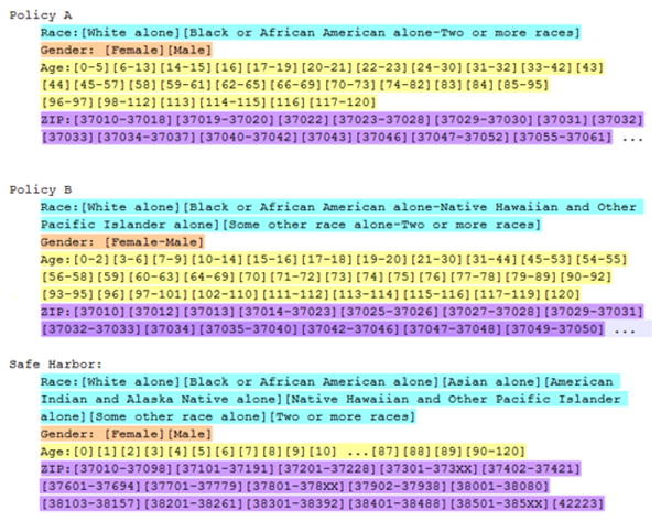
After investigating the policies which dominated Safe Harbor, we found that 23 of the policies were from one chain of the same sublattice. This observation indicates that the frontier policies found by SHS can provide a user with highly related policies which should be useful in practice. We show examples of policies that dominate Safe Harbor in Figure 9.⁵ Here, we illustrate through two policies (A and B), the actual semantic differences proposed by our discovered policies. We note that for brevity, we abbreviate the enumeration of ZIP code generalizations in both Policies A and B. We further note that Policy A is one policy in the previously mentioned group of 23 along the same chain, while Policy B is the lone unrelated policy. While each policy generalizes Age and ZIP to different levels, the primary difference is the generalization of Race and Gender. Where Policy A generalizes “Black or African American” with all other races, it leaves Gender unmodified. Policy B, however, generalizes “Black or African American alone” with “Asian”, “American Indian and Alaska Native alone”, and “Native Hawaiian and Other Pacific Islander alone”, while “Some other race alone” is generalized with “Two or more races”. While these policies differ greatly from that suggested by Safe Harbor, it is worth mentioning that these policies – again – strictly dominate Safe Harbor.

Figure 9. Examples of two policies (upper and middle) discovered by SHS that strictly dominate Safe Harbor (lower).

Additionally, we compared our algorithm to the method of Benitez et al. [6]. It can see in Figure 8(b) that [6] returns only policies with risk not greater than Safe Harbor, while our method returns the “best” alternatives discovered.

Indeed, while [6] yields 500 policies which dominate the Safe Harbor policy, 98% of these are dominated by the 24 policies we return as a part of our discovered frontier.

5. Discussion

5.1 Main Findings and Implications

In this work, we formalized the problem of de-identification policy frontier discovery (DPFD) as a dual-objective optimization. We demonstrated how to map the space of policy alternatives to a Risk-Utility (R-U) metric space for each given dataset, where a frontier represents a set of non-dominating policy tradeoffs. Given the complexity of the discovery task, we introduced a probability-driven heuristic search algorithm, whose effectiveness over an existing competitor strategy was verified through an empirical evaluation. We demonstrated that the heuristic enabled efficient construction of a frontier, but further showed that, for a dataset representative of the demographics of Tennessee, a common de-identification policy for health information is suboptimal to the frontier.

Although we cannot guarantee discovery of the optimal frontier, we believe there are several major benefits of our research. First, the fact that the policies in our frontier can dominate a broadly-adopted mainstream de-identification policy suggests that our approximate frontier is useful. We believe that a healthcare organization willing to follow the Safe Harbor policy can justify the use of an alternative on our frontier when it dominates in both risk and information loss. Second, we believe that our approach could be useful for assisting policy makers to reason about what might constitute a different de-identification standard. The visualization of the trade-off between privacy risk and information loss should assist in such decision making. For instance, our approach can demonstrate how small changes in risk (or information loss) could lead to significant gains in information loss (or risk). Third, we provide the visualization of R-U frontier to address the alternative policy set navigation issue in previous de-identification policy discovery methods such as [6]. A user can easily locate a policy that satisfies their R-U tradeoff preference through navigating the frontier.

5.2 Limitations and Next Steps

Despite its merits, there are several limitations of the work that we wish to highlight. First, our framework requires a complete ordering of the domain of QI attributes and a structuring of all policy alternatives in a lattice. Yet, some data publishers may want to measure the information loss or risk in a function that does not satisfy this limitation. At this time, it is unclear how partial orders of a domain could be explored through a systematic search. One concern in particular is that partial orders may violate the homomorphism requirement of the risk and information loss functions.

Second, our study uses specific risk and utility measures, which may not be desirable in all cases. For instance, our risk measure assumes each record contributes a risk proportional to its group size (e.g., an individual in a group size of one contributes an equal amount of risk as two individuals in a group size of two). This is not necessarily the case and alternative risk measures may be more appropriate for modeling [38]. Similarly, our utility is based on an information theoretic measure which characterizes the distance between the distribution of QI values in the original and de-identified dataset. It thus neglects the relationship between the QI attributes and additional information that may be disclosed (e.g., the diagnoses for a patient). We adopted this perspective because regulation (e.g., the HIPAA Privacy Rule) does not address this issue. We recognize that models exist for characterizing such a relationship (e.g., mutual information measures) and believe they are worth considering in the future.

Third, it is possible that our dataset is not properly representative. In our analysis, we analyzed demographics in Tennessee, but not other states or smaller locales (e.g., counties). To further evaluate the effectiveness of our approaches, we plan on performing empirical studies with additional populations in the US and abroad.

Finally, as mentioned earlier, our search algorithm does not provide any guarantees with respect to the optimal solution. We believe a fruitful research direction is in the definition of approximation algorithms for the discovery of the frontier. Such approximation strategies have been addressed for certain anonymization [2] problems and it is possible that similar approaches may be appropriate for de-identification.

6. Conclusions

Organizations that must publish person-specific data for secondary use applications need to make a tradeoff between privacy risks (R) and utility (U). To provide a guideline for data publishers to make this tradeoff, we 1) added a semantic utility metric to an alternative de-identification policy discovery framework, 2) mapped each policy to a two-dimensional R-U space, and 3) formalized the frontier search problem. To solve the problem, we build a set of policies that define a frontier in the R-U space through a heuristic search with a probabilistic basis. We demonstrated that our approach dominates a baseline approach in terms of the quality of the frontier obtained within a fixed number of searched policies.

Our empirical study on the Adult dataset, supplemented with population statistics from of the state of Tennessee showed that our method can efficiently find a frontier in the R-U space which dominates the commonly applied HIPAA Safe Harbor policy (i.e., less risk and more utility). We believe that the frontier can be used as a tool to assist data managers make informed decisions about the relationships between risk and utility when sharing data. Our frontier policy framework is highly generalizable in the sense that the risk and utility measures can be any function, provided 1) they satisfy certain order homomorphisms and 2) the policy space can be structured for a systematic search.

In future research, we anticipate investigating if other heuristic (or approximation) strategies could be invoked to discover better frontiers and assess if similar results are obtained through the study of other geographic locales.

Appendix

Appendix: Generating Sublattices for SHS

To ensure new regions in the lattice are explored, the SHS algorithm systematically generates sublattices which do not overlap with the list of pruned regions.

A Constraint Satisfaction Formulation

Given a list of pruned sublattices, we define the problem of generating the next sublattice to consider as a constraint satisfaction problem.

Based on the definition of a sublattice, each policy in a sublattice is bounded by the upper policy α and the lower policy β will have a set of bits in common. In particular,

$${\forall }_{\gamma }\left({\alpha }_i\in \mathit{\text{sublattice}}\left(\alpha ,\beta \right)\to \forall j\left(\alpha \left[j\right]=1\to \gamma \left[j\right]=1\right)\wedge \forall j\left(\beta \left[j\right]=0\to \gamma \left[j\right]=0\right)\right)$$

Now, let us assume {a₁, a₂, …, a_n2} and {b₁, b₂, …, b_n1} are the sets of bits set to 0 and 1 in all policies of the sub-lattice, respectively. For reference, assume B is a bit-string that represents a policy. A sublattice(α, β) can then be represented as a conjunction clause:

$$B\left[b_1\right]=1\wedge \cdots \wedge B\left[b_{n_1}\right]=1\wedge B\left[a_1\right]=0\wedge \cdots \wedge B\left[a_{n_2}\right]=0.$$

A sufficient condition for a sublattice to not to have any overlap with another sublattice is:

$$\neg (B\left[b_1\right]=1\wedge \cdots \wedge B\left[b_{n_1}\right]=1\wedge B\left[a_1\right]=0\wedge \cdots \wedge B\left[a_{n_2}\right]=0)$$

This condition is equivalent to:

$$B\left[b_1\right]=0\vee \cdots \vee B\left[b_{n_1}\right]=0\vee B\left[a_1\right]=1\vee \cdots \vee B\left[a_{n_2}\right]=1.$$

and is precisely the constraint defined by sublattice(α, β). For example, all policies in sublattice([0, 0, 0, 0, 1], [1, 0, 1, 0, 1]) satisfy B[4] = 1 ∧ B[3] = 0 ∧ B[3] = 0 As a result, the corresponding constraint clause is B[4] = 0 ∨ B[1] = 1 ∨ B[3] = 1.

Searching for Sublattices

Algorithm 3 summarizes the search process for non-overlapping lattices. Given a set of pruned sublattices, each one defines a clause. The conjunction of the set of clauses is the constraint which the new sublattice should satisfy. We assume the set of clauses is C = {c₀, …, c_m}, and each clause is a disjunction set of literals $c_i=\{l_i^0,\dots ,l_i^{n_i}\}$. If this constraint set is satisfiable, we can find a set of literals S = {s₀, …, s_ns}, such that s₀ ∧ ⋯ ∧ s_ns → c₀ ∧ ⋯ ∧ c_m.

We use a depth-first search to find a set of literals for which the conjunction satisfies the aforementioned requirement. We begin by randomly selecting a literal I from the clause with the least number of literals. We check each clause and if l → c₀ ∧ ⋯ ∧ c_m, then it is deemed a solution; otherwise, we add l to path, which keeps the solution set S, and keep searching.

In each iteration, we add a random literal from the clause with the least number of literals in the unsatisfied constraint clause by the current path to expand the path. Selecting the clause with the least number of literals is a greedy strategy.

Algorithm 3 Search Non-overlapping Lattices (SNL)
Input: Constraints, a list of clauses defined by the set of pruned sublattice
Output: path, a list of literals that defines a solution sub-lattice
1:	path ← ∅
2:	Stack ← ∅
3:	root ← shortestclause(Constraints)
4:	push(Stack,root)
5:	while Stack ≠ ∅ do
6:	clause ← pop(Stack)
7:	if clause ≠ ∅ then
8:	literal ← randomliteral(clause)
9:	remove(clause,literal)
10:	push(Stack,clause)
11:	if Conflict(literal,path)= TRUE then
12:	continue
13:	else
14:	push(path, literal)
15:	unsatisfied ← unsatisfied(Constraints, path)
16:	if unsatisfied = ∅ then
17:	return path
18:	else
19:	clause ← shortestclause(unsatisfied)
20:	push(Stack,clause)
21:	end if
22:	end if
23:	else
24:	if path ≠ ∅ then
25:	pop(path)
26:	end if
27:	end if
28:	end while
29:	return path

The process is relatively straightforward. Instead of proceeding through all of the details for the algorithm, we present an simple example. Assume the constraint set is:

$$\left(B\left[4\right]=1\right)\wedge \left(B\left[2\right]=0\vee B\left[4\right]=0\right)\wedge \left(B\left[1\right]=1\vee B\left[2\right]=0\vee B\left[3\right]=1\right)$$

Then, the complete search tree is depicted in Figure 10. Path = {B[4] = 1, B[2] = 0} is a possible solution.

Figure 10. The search tree of the constraint satisfaction problem defined by the pruned lattice set.

References

- 1.Directive 95/46/EC of the european parliament and of the council of 24 October 1995 on the protection of individuals with regard to the processing of personal data and on the free movement of such data, 1995
- 2.Aggarwal G, Feder T, Kenthapadi K, Motwani R, Panigrahy R, Thomas D, Zhu A. Anonymizing tables. Proceedings of the 10th International Conference on Database Theory; 2005. pp. 246–258. [Google Scholar]
- 3.Arzberger P, Schroeder P, Beaulieu A, et al. Science and government. An international framework to promote access to data. Science. 2004;303(5665):1777–1778. doi: 10.1126/science.1095958. [DOI] [PubMed] [Google Scholar]
- 4.Bayardo RJ, Agrawal R. Data privacy through optimal k-anonymization. Proceedings of the 21st International Conference on Data Engineering; 2005. pp. 217–228. [Google Scholar]
- 5.Belanger F, Hiller J, Smith W. Trustworthiness in electronic commerce: the role of privacy, security, and site attributes. Journal of Strategic Information Systems. 2002;11:245–270. [Google Scholar]
- 6.Benitez K, Loukides G, Malin B. Beyond safe harbor: automatic discovery of health information de-identification policy alternatives. Proceedings of the 1st ACM International Health Informatics Symposium; 2010. pp. 163–172. [DOI] [PMC free article] [PubMed] [Google Scholar]
- 7.Bughlin J, Chui M, Manyika J. Clouds, big data, and smart assets: ten tech-nabled business trends to watch. McKinsey Quarterly. 2010 Aug; [Google Scholar]
- 8.Ciriani V, di Vimercati SDC, Foresti S, Samarati P. k-anonymity. Secure Data Management in Decentralized Systems. 2007:323–353. [Google Scholar]
- 9.Dalenius T. Finding a needle in a haystack or identifying anonymous census records. Journal of Official Statistics. 1986;2:329–336. [Google Scholar]
- 10.Dewri R, Ray I, Ray I, Whitley D. On the optimal selection of k in the k-anonymity problem. Proceedings of the 24th IEEE International Conference on Data Engineering; 2008. pp. 1364–1366. [Google Scholar]
- 11.Duncan GT, Keller-Mcnulty SA, Stokes SL. Disclosure risk vs data utility: The R-U confidentiality map. National Institute for Statistical Science; Research Triangle Park, NC: Dec, 2001. Technical Report 121. [Google Scholar]
- 12.El Emam K. Heuristics for de-identifying health data. IEEE Security and Privacy. 2008;6(4):58–61. [Google Scholar]
- 13.El Emam K, Arbuckle L, Koru G, et al. De-identification methods for open health data: the case of the Heritage Health Prize claims dataset. Journal of Medical Internet Research. 2012;14(1):e33. doi: 10.2196/jmir.2001. [DOI] [PMC free article] [PubMed] [Google Scholar]
- 14.Frank A, Asuncion A. UCI machine learning repository. 2012 [Google Scholar]
- 15.Fung BCM, Wang K, Chen R, Yu PS. Privacy-preserving data publishing: A survey of recent developments. ACM Computing Surveys. 2010;42(4):14. [Google Scholar]
- 16.Fung BCM, Wang K, Yu PS. Top-down specialization for information and privacy preservation. Proceedings of the 21st International Conference on Data Engineering; 2005. pp. 205–216. [Google Scholar]
- 17.Hallinan D, Friedewald M, McCarthy P. Citizens' perceptions of data protection and privacy in europe. Computer Law and Security Review. 2012;28:263–272. [Google Scholar]
- 18.Hrynaszkiewicz I, Norton ML, Vickers AJ, Altman DG. Preparing raw clinical data for publication: guidance for journal editors, authors, and peer reviewers. BMJ. 2010;340:c181. doi: 10.1136/bmj.c181. [DOI] [PMC free article] [PubMed] [Google Scholar]
- 19.Iyengar VS. Transforming data to satisfy privacy constraints. Proceedings of the 8th ACM SIGKDD International Conference on Knowledge Discovery and Data Mining; 2002. pp. 279–288. [Google Scholar]
- 20.Kifer D, Gehrke J. Injecting utility into anonymized datasets. Proceedings of the ACM SIGMOD International Conference on Management of Data; 2006. pp. 217–228. [Google Scholar]
- 21.Lambert D. Measures of disclosure risk and harm. Journal of Official Statistics. 1993;9:313–331. [Google Scholar]
- 22.LeFevre K, DeWitt DJ, Ramakrishnan R. Mondrian multidimensional k-anonymity. Proceedings of the 22nd IEEE International Conference on Data Engineering; 2006. p. 25. [Google Scholar]
- 23.Li T, Li N. Towards optimal k-anonymization. Data Knowl Eng. 2008 Apr;65(1):22–39. [Google Scholar]
- 24.Li T, Li N. On the tradeoff between privacy and utility in data publishing. Proceedings of the 15th ACM SIGKDD International Conference on Knowledge Discovery and Data Mining; 2009. pp. 517–526. [Google Scholar]
- 25.Lohr S. The age of big data. New York Times; Feb 11, 2012. [Google Scholar]
- 26.Loukides G, Gkoulalas-Divanis A, Shao J. On balancing disclosure risk and data utility in transaction data sharing using R-U confidentiality map. Joint UNECE/Eurostat Work Session on Statistical Data Confidentiality. 2011:19. [Google Scholar]
- 27.Meyerson A, Williams R. On the complexity of optimal k-anonymity. Proceedings of the 23rd ACM Symposium on Principles of Database Systems; 2004. pp. 223–228. [Google Scholar]
- 28.Narayanan A, Shmatikov V. Myths and fallacies of “personally identifiable information”. Communications of the ACM. 2010;53(6):24–26. [Google Scholar]
- 29.National Institutes of Health. Policy for sharing of data obtained in NIH supported or conducted genome-wide association studies. 2002 Aug; NOT-OD-07-088. [Google Scholar]
- 30.Ohm P. Broken promises of privacy: responding to the surprising failure of anonymization. UCLA Law Review. 2010;57:1701–1777. [Google Scholar]
- 31.Olson JS, Grudin J, Horvitz E. A study of preferences for sharing and privacy. Proceedings of the CHI'05 Extended Abstracts on Human Factors in Computing Systems; 2005. pp. 1985–1988. [Google Scholar]
- 32.Rastogi V, Suciu D, Hong S. The boundary between privacy and utility in data publishing. Proceedings of the 33rd International Conference on Very Large Data Bases; 2007. pp. 531–542. [Google Scholar]
- 33.Samarati P, Sweeney L. Protecting privacy when disclosing information: k-anonymity and its enforcement through generalization and suppression. SRI Computer Science Laboratory; 1998. Technical Report SRI-CSL-98-04. [Google Scholar]
- 34.Schildcrout J, Denny J, Bowton E, et al. Optimizing drug outcomes through pharmacogenetics: a case for preemptive genotyping. Clinical Pharmacology and Therapeutics. 2012;92(2):235–242. doi: 10.1038/clpt.2012.66. [DOI] [PMC free article] [PubMed] [Google Scholar]
- 35.Schwartz P, Solove D. The PII problem: Privacy and a new concept of personally identifiable information. New York University Law Review. 2011;86:1814–1894. [Google Scholar]
- 36.Shlomo N. Statistical disclosure control methods for census frequency tables. International Statistical Review. 2007;75(2):199–217. [Google Scholar]
- 37.Shlomo N, Young C. Statistical disclosure control methods through a risk-utility framework; Proceedings of the 2006 CENEX-SDC project international conference on Privacy in Statistical Databases, PSD'06. Berlin, Heidelberg. 2006. pp. 68–81. [Google Scholar]
- 38.Skinner C, Elliot M. A measure of disclosure risk for microdata. Journal of the Royal Statistical Society. 2002;64:855–867. [Google Scholar]
- 39.Sweeney L. Achieving k-anonymity privacy protection using generalization and suppression. International Journal on Uncertainty, Fuzziness and Knowledge-based Systems. 2002;10:571–588. [Google Scholar]
- 40.Sweeney L. k-anonymity: a model for protecting privacy. International Journal on Uncertainty, Fuzziness and Knowledge-based Systems. 2002;10(5):557–570. [Google Scholar]
- 41.Tene O, Polonetsky J. Privacy in the age of big data. Stanford Law Review Online. 2012;64:63–69. [Google Scholar]
- 42.Trottini M, Fienberg SE. Modelling user uncertainty for disclosure risk and data utility. International Journal of Uncertainty, Fuzziness and Knowledge-Based Systems. 2002 Oct;10(5):511–527. [Google Scholar]
- 43.Truta TM, Fotouhi F, Barth-Jones D. Disclosure risk measures for microdata. Proceedings of the 15th International Conference on Scientific and Statistical Database Management; 2003. pp. 15–22. [Google Scholar]
- 44.U.S. Census Bureau. American fact finder. 2012 website: http://www.americanfactfinder.gov.
- 45.U.S. Department of Health & Human Services. Standards for privacy of individually identifiable health information, final rule, 45 CFR, pt 160-164. 2002 Aug; [PubMed] [Google Scholar]
- 46.Walport M, Brest P. Sharing research data to improve public health. Lancet. 2011;377(9765):537–539. doi: 10.1016/S0140-6736(10)62234-9. [DOI] [PubMed] [Google Scholar]