

Abstract
The spatial pattern of the uncertainty in air pollution-related health impacts due to climate change has rarely been studied due to the lack of high-resolution model simulations, especially under the Representative Concentration Pathways (RCPs), the latest greenhouse gas emission pathways. We estimated future tropospheric ozone (O3) and related excess mortality and evaluated the associated uncertainties in the continental United States under RCPs. Based on dynamically downscaled climate model simulations, we calculated changes in O3 level at 12 km resolution between the future (2057–2059) and base years (2001–2004) under a low-to-medium emission scenario (RCP4.5) and a fossil fuel intensive emission scenario (RCP8.5). We then estimated the excess mortality attributable to changes in O3. Finally, we analyzed the sensitivity of the excess mortality estimates to the input variables and the uncertainty in the excess mortality estimation using Monte Carlo simulations. O3-related premature deaths in the continental U.S. were estimated to be 1,312 deaths/year under RCP8.5 (95% confidence interval (CI): 427 to 2,198) and −2,118 deaths/year under RCP4.5 (95% CI: −3,021 to −1,216), when allowing for climate change and emissions reduction. The uncertainty of O3-related excess mortality estimates was mainly caused by RCP emissions pathways. Excess mortality estimates attributable to the combined effect of climate and emission changes on O3 as well as the associated uncertainties vary substantially in space and so do the most influential input variables. Spatially resolved data is crucial to develop effective community level mitigation and adaptation policy.
Keywords: climate change, ozone, mortality, uncertainty, Representative Concentration Pathways (RCPs), spatial variation
1 Introduction
Climate change, such as changes in air temperature, precipitation and air circulation, and emission change, can affect the chemical reactions in both gas phase and aerosols; and thus may further impact air quality. In particular, tropospheric ozone (O3) has been of concern in the context of climate change because the production of secondary air pollutants depends strongly on meteorological conditions. Exposure to elevated O3 concentrations have been associated with excess mortality (EM), including respiratory and cardiovascular mortality (Bell et al. 2004; Jerrett et al. 2009; Levy et al. 2005).
Previous studies have estimated air pollution-related health impacts due to future climate change (Bell et al. 2007; Chang et al. 2010; Jackson et al. 2010; Knowlton et al. 2004; Post et al. 2012; Tagaris et al. 2009). For example, Bell et al. (2007) found that O3 levels are estimated to increase under the Intergovernmental Panel on Climate Change (IPCC) Special Report on Emissions Scenarios (SRES)-A2 scenario, with the largest increases in cities with present-day high O3 pollution. The elevated O3 levels correspond to approximately a 0.11% to 0.27% increase in daily mortality for 50 cities in the United States (U.S.). Knowlton et al. (2004) found a median 4.5% increase in O3-related acute mortality in New York City and the surrounding counties under the SRES-A2 scenario. Post et al. (2012) addressed a wide range of O3-related health effects, from roughly 600 deaths avoided to 2,500 deaths attributable to climate change in the U.S.; the heath impact varied by modeling choices for O3 concentration simulation, as well as by assumptions for future climate and population change. Using the SRES-A1B scenario, the same population, and the same air pollutants emissions as in 2001, Tagaris et al. (2009) found that the O3 change due to future climate change could cause an increase in annual premature deaths by 300 deaths in 2050 across the continental U.S.
However, the studies reported so far have a few limitations. First, few studies have comprehensively investigated the uncertainty of air pollution-related EM estimates reflecting all possible sources. Knowlton et al. (2004) performed sensitivity analyses focusing on emission change, population growth, and subsequent O3 change. Post et al. (2012) investigated the sensitivity of their estimates to modeling choices for the simulation of future O3 levels and reported national-level results. The uncertainties of EM estimates related to air quality changes due to climate change can be attributed to various factors, such as greenhouse gas (GHG) emissions scenarios, model performances, concentration-response functions (CRF), population growth, spatial domain, grid resolution, periods modeled, and mortality rates, all of which may vary in space. Therefore, uncertainty analyses, including all the variables associated with health risks due to future climate change and considering the spatial variation of the uncertainties, should be taken into account.
Second, the estimated impacts on population health can be significantly influenced by emission scenarios. To date, few studies have evaluated the health impact of future O3 concentration changes based on the latest GHG emission scenarios, i.e., the Representative Concentration Pathways (RCPs) (Moss et al. 2010; Van Vuuren et al. 2011). As a set, the RCPs cover a range of forcing levels associated with emission scenarios published in the literature, representing present and planned air quality legislation for the projection of regional air pollutant emissions, as well as GHG atmospheric concentrations. Therefore, the combined effect of air pollutant emissions and GHG concentration changes on air quality could differ from previous studies based on SRES and subsequently result in a different health impact. West et al. (2013) simulated the co-benefits of global GHG reductions on air quality and human health based on RCP4.5. However, the study focused on the effect of GHG reductions at the global and regional scales, and neither analyzed the uncertainty of the estimated EMs, nor estimated community-specific EMs.
Finally, few studies have analyzed the distribution of the estimated impacts of O3 at a fine spatial scale over a large region. Bell et al. (2007) presented O3-related mortality covering 50 cities in the U.S., but did not focus on the spatial variation of EM. Post et al. (2012) also did not analyze the spatial variation of O3-related health impacts of climate change, but focused on the variation of health impacts related to modeling choices. Tagaris et al. (2009) presented spatially resolved O3-related EM, but only state-level estimates were reported. The most recent study by West et al. (2013) is based on the spatial resolution of 2°×2.5°, which is far beyond community size.
In this analysis, we applied high-resolution climate model simulations to project the change in O3 levels under two RCP emission pathways over the entire continental U.S. Then, we calculated the change of county-level EM due to exposure to O3 in the future (2057–2059) from the base years (2001–2004). Finally, we characterized the uncertainty in the health impact estimates through each stage of health risk modeling.
2 Methodology
2.1 Air quality simulations
A coupled global and regional climate modeling system was developed to provide 2001–2004 and 2057–2059 air pollution levels in the continental U.S. at 12 km resolution. The configuration and evaluation of this system are briefly described here (More details are addressed in our previous study, Gao et al. 2013). The state-of-the-art earth system model Community Earth System Model version 1.0 (CESM1.0), developed at the National Center for Atmospheric Research (NCAR), can simultaneously simulate the Earth’s atmosphere, ocean, land surface, and sea-ice (Gent et al. 2011). In this study, the atmospheric chemistry was integrated with the atmospheric component, Community Atmosphere Model, referred to as the CAM-Chem (Lamarque et al. 2012). CESM/CAM-Chem was used in the long-term global climate and chemistry simulations, from 1850 to 2005 as present climate and 2005 to 2100 for RCP4.5 and RCP8.5, with a spatial resolution of 0.9° (latitude) ×1.25° (longitude). The CESM-projected meteorological fields were used as the initial and boundary conditions of the regional climate model, Weather Research and Forecasting model (WRF) 3.2.1 (Skamarock and Klemp 2008). Chemical species simulated by the atmospheric chemistry component of the CESM/CAM-Chem were mapped to the regional air quality model, Community Multi-scale Air Quality Model version 5.0 (CMAQ 5.0; Wong et al. 2012).
We selected RCP4.5 and RCP8.5 to evaluate and compare future O3 level and its related health impact. RCP4.5 corresponds to the stabilization of radiative forcing at 4.5 W/m2 in the year 2100 without ever exceeding that value, and it assumes a lower population growth rate, high income, and rapid technology development (Thomson et al. 2011). RCP8.5 is a high-GHG emission pathway corresponding to the stabilization of radiative forcing at 8.5 W/m2 in the year 2100, and it assumes high population growth rate, lower income, and lower technology development rate in developing countries (Riahi et al. 2011). The emissions trends in the RCPs are mainly controlled by the driving forces (population, income, energy use, etc.), climate policy, and air pollution control policy (Van Vuuren et al. 2011). In terms of climate policy, RCP4.5 has more stringent GHG emissions control, while RCP8.5 assumes no climate policy, even though both scenarios are projected to increase the use of renewable resources. Unlike the SRES scenarios, where anthropogenic emissions related to air pollutants have a modest decrease or even increase (under A1FI), all RCPs include stringent air pollution control policies with any increase in income. Thus, under the RCPs, O3 precursors including carbon monoxide (CO), nitrogen oxides (NOx), and non-methane volatile organic compounds (NMVOCs), are projected to decrease in the U.S. (See Table 2 in Gao et al. (2013) for projection factor for anthropogenic emissions). However, the GHG emissions increase, particularly the methane concentrations under RCP8.5, will negatively affect O3 air quality. As a result, the projected O3 levels in 2057–2059 in this study reflect the influence of both climate change and emissions control on O3 precursors.
Using CMAQ-simulated hourly O3, we computed annual means of maximum daily 8-hour average O3 (MDA8 O3) and maximum daily 1-hour average O3 (MDA1 O3) for each 12 km grid cell. We then aggregated the 12×12 km grid of O3 concentration to the county level (3,109 counties in the continental U.S.). We determined the population-weighted centroid of each county and then averaged the data in the nine grid cells closest to the centroid. We calibrated the simulated O3 level for bias reduction. To compare the CMAQ-simulated values with observations at the county level, we used monitored data from the U.S. Environmental Protection Agency (USEPA) Air Quality System (USEPA-AQS) and the Environmental Benefits Mapping and Analysis Program Community Edition 1.0.8 (BenMAP-CE) developed by the USEPA (USEPA 2012). Using BenMAP-CE, we calculated county-level O3, applying the Voronoi neighbor averaging algorithm, which interpolates monitored O3 data to unmonitored locations. BenMAP-CE first identifies the set of monitors that best “surround” the population center of the grid cell and then takes an inverse-distance weighted average of the monitoring values (Fann et al. 2012; USEPA 2012). We matched the CMAQ-simulated values with the interpolated, county-level observations for 2001–2004. After calculating the county-level ratios of CMAQ simulations over observations in the base years, we calibrated the CMAQ-simulated MDA8 O3 and MDA1 O3 concentrations for both 2001–2004 and 2057–2059 using these calibration ratios for each county (Figure S1, Supplementary Material).
2.2 Projection of future population
The county-level population projections for 2055 were taken from the Integrated Climate and Land-Use Scenarios (ICLUS) project (USEPA 2009). The ICLUS population projections were based on a standard cohort-component method, in which the initial U.S. population in 2005 was divided into age-, gender-, and race/ethnicity-specific cohorts. Cohort size was estimated over time separately for each cohort, with various scenarios regarding fertility, mortality, and migration (Preston et al. 2001). In ICLUS, four scenarios were considered: A1, low fertility, high net domestic migration, and high net international migration; B1, low fertility, low net domestic migration, and high net international migration; A2, high fertility, high net domestic migration, and medium net international migration; and B2, medium fertility, low net domestic migration, and medium net international migration, with the categories (i.e., low, medium, and high) defined in the IPCC-SRES. Mortality rate was kept constant across all scenarios because the U.S. Census Bureau did not release alternative scenarios for mortality rates. Although the four ICLUS scenarios did not cover the widest possible range of population size, they represented combinations of potential fertility, mortality, and migrations in the future. A more detailed discussion on ICLUS population projection was presented elsewhere (USEPA 2009).
2.3 Excess mortality due to exposure to air pollution
To calculate baseline future mortality incidence without the impact of climate and O3 precursors changes, we used predicted county-specific mortality rates adopted in BenMAP-CE, which is derived from a projected, age-specific ratio of the 2050 mortality rate to the 2005 mortality rate. The mortality rates do not, however, explicitly account for climate change. The basis for the future mortality rate projection is described in detail elsewhere (USEPA 2012). We used non-accidental, all-cause mortality to be consistent with the CRF used in this study.
To calculate EM due to O3 exposure, we based the CRFs on the association between non-accidental, all-cause mortality and short-term exposure to MDA8 O3 (Bell et al. 2004) and MDA1 O3 (Bell et al. 2004; Levy et al. 2005). Bell et al. (2004) analyzed the relationship between O3 and non-accidental, all-cause mortality using the National Morbidity, Mortality, and Air Pollution Study (NMMAPS) dataset, which covers 95 U.S. cities. Levy et al. (2005) derived the relative risk from meta-analyses of 27 studies for North America. There might be publication bias in the meta-analyses results. Nevertheless, the cities chosen in these studies have a wide range of O3 concentrations and represent both rural and urban populations. We therefore applied the CRF coefficients in Bell et al. (2004) and Levy et al. (2005) (Table S1, Supplementary Material).
Finally, we estimated the change in county-level EM as follows (Fann et al. 2012; Post et al. 2012):
| (1) |
where Δy is the expected number of deaths per year attributable to changing O3 level at county i; POPi is population in county i; MRi is population mortality rate; POPi×MRi indicates baseline mortality incidence (i.e., assuming no climate change and O3 precursors emission change); β is the coefficient of the concentration-response function for O3; ΔCi is the concentration difference of O3 between 2057–2059 and 2001–2004.
We estimated EM for non-accidental, all-cause mortality associated with O3 for both year round and warm season (May through September). Lastly, we analyzed the spatial variation of EM by county and the nine climate regions defined by the National Climatic Data Center (http://www.ncdc.noaa.gov/temp-and-precip/us-climate-regions.php) (Fig. 1).
Fig. 1.
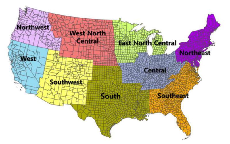
Nine climate regions in the United States
2.4 Sensitivity and Uncertainty analyses
To determine the sensitivity of the EM to various factors (i.e., two RCPs, four future population projections, and three CRF coefficients), we conducted an analysis of variance (ANOVA) for EM estimates to decompose the total variability in estimated EM into the contribution of each factor. In contrast to the approach in a previous study (Post et al. 2012) which used national-level EM estimates, we conducted the ANOVA by county and then calculated the county-level percentage of sum of squares (SS) for RCPs, population projections, and CRF coefficients. We also plotted the county-level percentage of SS to visually analyze the spatial distribution of the sensitivity to the factors.
The ANOVA apportions the variability in the mean estimated air pollution EM in each county to the mean levels of each factor in Equation 1 without considering their uncertainties (i.e., each factor has a distribution of possible values). We used Monte Carlo simulations to evaluate the uncertainty of EM estimates attributable to the ranges of CRF coefficients, mortality rates, and concentration changes of O3. CRF coefficients and mortality rates are assumed to be normally distributed with independent, county-specific means and standard errors. As there is no standard error for the projected 2050 mortality rate, we used the standard error for the year 2009 at the county level provided by the Centers for Disease Control and Prevention (CDC 2012). For concentration changes of O3, triangular-distributed random variables were generated using the minimum, maximum, and mean of three annual mean values. Random sampling and EM calculations were repeated 1,000 times for each county. Then, we computed the Monte Carlo means and standard errors of the 1,000 EM estimates by county. By summing all the county-level EMs derived from the Monte Carlo simulations, we estimated national-level EM estimates and their 95 % confidence intervals (CIs). We also calculated the probability distributions of all the national EM due to future O3 change.
3 Results
3.1 O3 change
The spatial distributions of county-level O3 change between the future (2057–2059) and the base years (2001–2004) are shown in Figure 2. Projected O3 concentrations by climate region are presented in Supplementary Material, Table S2. Changes in estimated county-level MDA8 O3 ranged from −8.8 to 7.5 ppb under RCP4.5 and from −3.6 to 11.5 ppb under RCP8.5 across 3,109 counties. Higher O3 increases in the Northwest, West, and West North Central region are likely caused by higher background O3 in the spring and winter, as well as an increase of methane emissions in RCP8.5 (Gao et al. 2013). Nationally, O3 was projected to decrease under RCP4.5 and to increase under RCP8.5. However, O3 levels of most counties in the Northwest, West North Central, and West region were projected to increase under RCP8.5 (Fig. 2(a)). Even under RCP4.5, some counties were expected to have higher O3 levels (Fig. 2(b)).
Fig. 2.
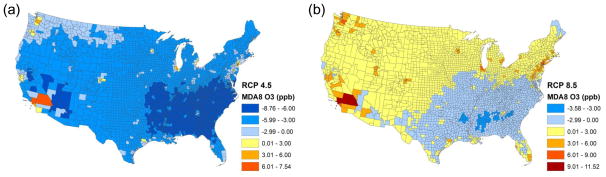
Spatial distribution of O3 changes between 2001–2004 and 2057–2059 (a) and (b) are MDA8 O3 changes for year round under RCP4.5 and 8.5, respectively
3.2 O3-related excess mortality
Table 1 shows the estimated national-level O3-related EM changes between 2001–2004 and 2057–2059 under the two RCPs. We derived national EM estimates in Table 1 from the summation of county-level EMs for each ICLUS population scenario and the average of the four ICLUS-based national EMs. Our 95% CIs in Table 1 are based on 4,000 national-level EMs (1,000 times of Monte Carlo simulations for four population projections) for each RCP. O3-related EMs vary by emission pathway, population projection, and CRF. Under RCP8.5, increased MDA8 O3 resulted in ~1,900 (95% CI: 1,700 to 2,100) premature deaths per year nationwide, when county-level EMs derived from the Monte Carlo simulation were summed using the four population projections in 2057–2059 and CRF from Bell et al. (2004). In contrast, decreased MDA8 O3 under the RCP4.5 resulted in the avoidance of ~1,600 (95% CI: 1,300 to 1,800) deaths per year. Projected county-level baseline mortality incidence for 2055 is shown in Supplementary Material, Figure S2. During the warm season, lower future MDA8 O3 levels could result in ~2,400 (95% CI: 2,100 to 2,700) avoided premature deaths under RCP4.5 (Table 1). Most of the counties would see a decrease in all-cause mortality under both RCPs, mainly as a result of lower O3 levels, while some counties in the West and Northwest would see an increase due to higher O3 levels (Supplementary Material, Figure S3(a) and (b)). Decreases in the EMs under RCP8.5 during the warm season, unlike year-round mortality, are related to decreases in O3 in summer. In other seasons, increases in EMs are due to higher O3 under RCP8.5 (Gao et al. 2013).
Table 1.
Ozone-related excess mortality at the national level due to future climate and emission changes (2057–2059) compared with baseline climate (2001–2004) under the two Representative Concentration Pathways (RCPs) (deaths per year)a
| Source of CRF coefficient | RCP4.5 Mean (95% CI)b |
RCP8.5 Mean (95% CI) |
|
|---|---|---|---|
| Year-round | Bell et al. (2004) (8hr) | −1,568 (−1,804, −1,332) | 1,930 (1,723, 2,137) |
| Bell et al. (2004) (1hr) | −2,153 (−2,438, −1,868) | 900 (778, 1,025) | |
| Levy et al.(2005) (1hr) | −2,634 (−2,977, −2,291) | 1,104 (986, 1,222) | |
| Warm season (May–September) | Bell et al. (2004) (8hr) | −2,401 (−2,674, −2,127)c | −470 (−556, −385) |
| Bell et al. (2004) (1hr) | −2,326 (−2,587, −2,064) | −626 (−720, −533) | |
| Levy et al.(2005) (1hr) | −5,817 (−6,469, −5,164) | −1,566 (−1,794, −1,340) |
Values are the averages of four population projections;
95% confidence intervals based on means and standard errors of national-level EM estimates obtained from the summation of county-level EMs under four population scenarios;
The O3-related EMs for warm season are greater than those for year-round, mainly because O3 concentration changes for the warm season are greater than those year-round.
County-level, O3-related EM estimates had high spatial variation (Fig. 3). Under RCP8.5, most counties in the Northwest, West North Central, and West were estimated to have an increased O3-related EM. Counties with a high population, such as Los Angeles County in California and Cook County in Illinois, showed higher increases in O3-related EM. The EMs in these counties appeared to increase even under RCP4.5 (Fig. 3(a)), despite the overall reduction in O3-related EM (Table 1). The spatial distribution for O3-related EM per 100,000 persons was different from that of the absolute values showing greater spatial heterogeneity. All counties in the Northwest showed higher increases in O3-related EM per 100,000 persons whereas many counties in the South and Southeast had decreased rates under RCP8.5 (Fig. 3(c)). The standard errors of county-level EM estimates also had high spatial variations as presented in Fig. 3(d) and (e) with Southern California showing the greatest standard errors.
Fig. 3.

Spatial distribution of excess mortality in 2057–2059 attributable to O3 changes (a) and (b) indicate annual of MDA8 O3–related EMs based on mortality risk from Bell et al. (2004) under RCP4.5 and RCP8.5, respectively (c) is EMs per 100,000 persons due to MDA8 O3 change under RCP8.5 (d) and (e) are the standard errors (SEs) of county-level EM estimates The means and SEs of EMs are derived from 1,000 Monte Carlo simulations of mortality rate, concentration change, and CRF coefficient Each county-level EM is obtained from the average of four EMs from four ICLUS population scenarios
3.3 ANOVA analysis
Table 2 shows the percentage contribution of county-level SS from factors in Equation 1 (i.e., CRF coefficient, population, and RCP) to the total SS based on the ANOVA analysis. A greater percentage reflects higher sensitivity of the EM to a specific factor. Overall, O3-related EM estimates were the most sensitive to the RCP, which account for almost 80% of the total SS.
Table 2.
ANOVA results for the percentage variance in estimated county-level excess mortality explained by various factors (%)a
| Population Mean (SD)b |
RCP Mean (SD) |
CRF Mean (SD) |
Residuals Mean (SD) |
|
|---|---|---|---|---|
| Year-round | 11.2 (13.2) | 79.5 (16.6) | 2.3 (2.9) | 6.9 (5.5) |
| Warm season (May–September) | 15.0 (13.7) | 35.5 (16.6) | 36.9 (14.7) | 12.6 (4.1) |
Four population scenarios, two Representative Concentration Pathways (RCPs), and three concentration-response functions (CRFs);
Standard deviation of county-level proportions (%)
However, factor contributions also vary widely in space (Fig. 4). Counties in the Northwest, West North Central, West, and Southwest had higher sensitivity to the RCP scenarios (Fig. 4(a)), since the projected O3 levels in these regions switched from a projected decrease under RCP4.5 to an increase under RCP8.5 (Fig. 2(a) and (b)). In contrast, counties in the Central, South, and Southeast had a higher sensitivity to the population projections.
Fig. 4.

County-level analysis of variance (ANOVA) results (a), (b), and (c) indicate the percent proportion of the sum of squares of emission pathway (RCP), concentration-response function (CRF), and population scenario (POP) to cover the variance of mean EM attributable to O3 change, respectively
3.4 Uncertainty analyses
Figure 5 shows the probability distribution of the estimated, national-level O3-related EMs (the national EM is the sum of county-level EMs and each scenario has 1,000 national EM estimates based on the county-level Monte Carlo simulations), accounting for MDA8 O3 and MDA1 O3, two different CRF coefficients, and four population scenarios. O3-related EMs ranged from 427 to 2,198 (95% CI) deaths per year, with a mean of 1,312 deaths per year under RCP8.5; and from −3,021 to −1,216 (95% CI) deaths per year, with a mean of −2,118 deaths per year under RCP4.5. The RCPs played a critical role in estimated, O3-related EM because O3 levels were found to increase under RCP8.5 in 2057–2059, but decrease under RCP4.5 compared with 2001–2004. The probability distribution of the estimated national EM is not smooth because of discrete population projections, averaging hours, and CRF ranges, but its two distinct modes follow the RCPs (Fig. 5(a)). The combined probability distribution function from the two RCPs predicts a ~50% chance that national O3-related EM will be greater than the base years, and a ~10% chance that O3-related EM in the future will be over 1,900 deaths per year more than the base years (Fig. 5(b)).
Fig. 5.

Probability distribution of all possible excess mortalities due to O3 changes under RCP4.5 and 8.5 (a) Probability distribution; (b) Cumulative distribution of the excess mortality
4 Discussion
Our results based on high-resolution climate model simulations illustrate that the effect of O3 change on mortality varies by emissions pathway, population projection, and CRF. Even within the same RCP and population scenario, the estimated EMs appear to vary substantially in space as both simulated O3 level and baseline mortality incidence vary by community. The large spatial variability emphasizes that assessments of the health effect of future O3 change caused by climate change and emission policy should be spatially resolved so that the mitigation and adaptation policy developed based on these assessments can be more cost effective.
Our results from the combined effect of climate change and emissions reductions on O3 precursors are consistent with a previous study by Tagaris et al. (2007), which reported decreases in mean summer MDA8 O3 concentrations when both climate change under the SRES A1B scenario and reductions in air pollutant emissions were considered. The results of the current study also demonstrate that future O3 level during the warm season will decrease under the RCPs because of the emission reduction for O3 precursors planned in the U.S., which resulted in avoided adverse health effects of potential climate change-induced O3 increase.
Annual changes in O3 levels between 2057–2059 and 2001–2004 showed dramatic differences between the two RCPs (i.e., the increase under RCP8.5 and decrease under RCP4.5). The projected emissions in RCPs consider both GHGs changes and air pollution control policies (Moss et al. 2010; Van Vuuren et al. 2011). The GHG emission scenarios based on the RCPs are comparable with SRES scenarios. For example, the CO2 concentrations in RCP4.5 and RCP8.5 are close to SRES B1 and A1FI, respectively (Meehl et al. 2011). The air pollutant emissions under SRES are projected to decrease only slightly or, depending on the emissions scenario, even increase. However, the RCPs assume that by the end of 2050s, CO is projected to decrease by more than 70% under both RCPs, and NMVOC and NOx by almost 70% and 50% under RCP8.5 and 40% and 60% under RCP4.5 in the U.S., respectively (Gao et al. 2013). On the other hand, methane emissions are predicted to increase by 61% in 2050s under RCP8.5, compared to 2005, whereas it would decrease by 10% under RCP4.5 (Gao et al. 2013). Such differences in methane mixing ratios under the two RCPs will affect O3 levels more greatly than the difference in NOx emissions (Lamarque et al. 2011). West et al. (2013) also pointed out that O3 reduction is largely (89%) due to co-emitted air pollutants in 2100, with only 11% explained by the change in meteorology due to climate change; and is strongly influenced by the decrease in methane emissions under RCP4.5. Therefore, we can infer that the increase in annual O3 under RCP8.5, despite the decrease in other O3 precursors, is mainly caused by the increase in future methane emissions.
Annual changes in O3 levels between the present and the future vary substantially by region. Under RCP8.5, O3 levels in the Northwest, West, and West North Central were projected to increase more than the other regions (e.g., an annual increase of 2.6 ppb in MDA8 O3 in the Northwest (Supplementary Material, Table S2)), resulting in more O3-related EM (Fig. 2(b) and Fig. 3(b)). Both the sensitivity and the uncertainty of the EM estimates also vary by region. The dramatic changes in annual O3 between RCPs played a critical role in the high sensitivity of O3-related EM to RCP. The high sensitivity of O3-related EMs to the RCPs could be related to the strong dependence of O3 production on temperature (Seinfeld and Pandis 2006) as well as the methane emission difference between the two RCPs.
A major strength of our study was our use of O3 simulations at a high resolution (i.e., 12×12 km). We analyzed county-level spatial variations and uncertainty of the EM due to emissions changes, as well as climate change. Previous studies were mostly based on coarser spatial resolutions (e.g., 36×36 km). By providing a better representation of the atmospheric circulation and topographical features, our high-resolution simulations generated more accurate O3 levels. Furthermore, we considered several possible sources of uncertainty, including RCP-based O3 change, population growth, mortality rate, and CRF. The framework to analyze the uncertainty of health effect of climate change proposed in this study can be utilized in decision support for developing both national and community level adaptation policy. To the best of our knowledge, this is the first RCP-based uncertainty analyses on the health impacts of air pollution change.
Our study has a few limitations. First, limited by computational resources, we did not consider differences between model systems to predict climate and O3 changes in the sensitivity analyses. It is related to high resolution model simulations which our analyses are based on and to the fact that there are very limited applications of dynamical downscaling under the new RCPs until now (Gao et al. 2013). As a result, our findings do not reflect the uncertainty related to using different climate models. Second, we used CRFs derived from short-term exposures to O3, as there are currently no epidemiological data based on long-term effects for all-cause mortality with statistical significance. However, the effects of short- and long-term O3 exposure on all-cause mortality will remain unclear until epidemiological research investigates the association of all-cause mortality to long-term O3 exposure (Fann et al. 2012). When we assessed the uncertainty from CRFs in the Monte Carlo analysis, we gave each study equal weight. This could artificially inflate our final uncertainty estimates. Thirdly, only three future years (2055–2057) were simulated for future O3 changes in this study due to limited computational resources. More studies including more years are required in the future. Lastly, it would be more appropriate to sum estimated daily excess mortality over the years than to estimate based on annual averaged O3 changes since the CRFs are based on daily data. However, because CMAQ-simulated O3 is driven by climate projections, daily O3 levels have too much uncertainty and daily-level calibration of future O3 levels is not meaningful. Further investigation is needed to determine the impact of our simplified method on the EM estimates.
5 Conclusions
Using the latest emissions pathways (RCPs), which reflect both planned air quality legislation and GHG emission changes for the future, we analyzed county-level O3-related EMs attributable to O3 changes in the late 2050s and their related uncertainties. The importance of spatially resolved analysis is demonstrated in our O3-related EM estimates. County-level, O3-related EM estimates have a wide spatial variation, ranging from positive to negative values and depending on the RCP and region. When both RCPs are considered together, the probability of climate change causing a more substantial public health impact (e.g. over 1,900 excess deaths nationwide) is not trivial, and this burden will fall disproportionally on the Northwestern U.S. Furthermore, regardless of the reduction in emissions of some O3 precursors, O3-related EM may still increase in the U.S. under RCP8.5, a fossil fuel intensive scenario. To prevent the potential adverse health effects due to O3-level increases triggered by climate change, it is necessary to rigorously mitigate GHGs and O3 precursor emissions in order to obtain a lower-carbon dependent future.
The uncertainties in the estimated EM are driven by the emission changes described in the RCPs, epidemiological studies, and population projections, all of which include a wide range of possible values to date. Because the contribution and importance of each factor varies spatially, a comprehensive evaluation of the uncertainties covering all input variables is necessary to produce a quantitative health impact assessment of climate change. Future research should also focus on gaining a better understanding of these factors to develop more effective mitigation strategies.
Supplementary Material
Acknowledgments
This study was supported by the Centers for Disease Control and Prevention (CDC) (Grant No. 5 U01 EH000405) and by the National Institutes of Health (NIH) (Grant No. 1R21ES020225). National Science Foundation through TeraGrid resources provided by National Institute for Computational Sciences (NICS) (TG-ATM110009 and UT-TENN0006) and resources of the Oak Ridge Leadership Computing Facility at the Oak Ridge National Laboratory supported by the Office of Science of the U.S. Department of Energy (DEAC05-00OR22725) were used for the climate and air pollution model simulations. Yang Gao was partly supported by the Office of Science of the U.S. Department of Energy as part of the Regional and Global Climate Modeling Program. The Pacific Northwest National Laboratory is operated for DOE by Battelle Memorial Institute (DE-AC05-76RL01830).
References
- Bell ML, McDermott A, Zeger SL, Samet J, Dominici F. Ozone and short-term mortality in 95 US urban communities, 1987–2000. JAMA. 2004;292(19):2372–2378. doi: 10.1001/jama.292.19.2372. [DOI] [PMC free article] [PubMed] [Google Scholar]
- Bell ML, Goldberg R, Hogrefe C, et al. Climate change, ambient ozone, and health in 50 US cities. Climatic Change. 2007;82(1):61–76. [Google Scholar]
- Centers for Disease Control and Prevention (CDC), National Center for Health Statistics. [Accessed 27 November 2012];Wide-Ranging On Line Data for Epidemiologic Research (WONDER) 2012 http://wonder.cdc.gov.
- Chang HH, Zhou J, Fuentes M. Impact of climate change on ambient ozone level and mortality in Southeastern United States. Int J Environ Res Public Health. 2010;7:2866–2880. doi: 10.3390/ijerph7072866. [DOI] [PMC free article] [PubMed] [Google Scholar]
- Fann N, Lamson AD, Anenberg SC, Wesson K, Risley D, Hubbell BJ. Estimating the national public health burden associated with exposure to ambient PM2.5 and ozone. Risk Anal. 2012;32(1):81–95. doi: 10.1111/j.1539-6924.2011.01630.x. [DOI] [PubMed] [Google Scholar]
- Gao Y, Fu JS, Drake JB, Lamarque JF, Liu Y. The impact of emission and climate change on ozone in the United States under representative concentration pathways (RCPs) Atmos Chem Phys. 2013;13:9607–9621. doi: 10.5194/acp-13-9607-2013.. [DOI] [PMC free article] [PubMed] [Google Scholar]
- Gent PR, Danabasoglu G, Donner LJ, et al. The Community Climate System Model version 4. J Climate. 2011;24:4973–4991. [Google Scholar]
- Jackson JE, Yost MG, Karr C, et al. Public health impacts of climate change in Washington State: projected mortality risks due to heat events and air pollution. Climatic Change. 2010;102:159–186. doi: 10.1007/s10584-010-9852-3. [DOI] [Google Scholar]
- Jerrett M, Burnett RT, Pope CA, et al. Long-term ozone exposure and mortality. N Engl J Med. 2009;360:1085–95. doi: 10.1056/NEJMoa0803894. [DOI] [PMC free article] [PubMed] [Google Scholar]
- Knowlton K, Rosenthal JE, Hogrefe C, et al. Assessing ozone-related health impacts under a changing climate. Environ Health Perspect. 2004;112:1557–1563. doi: 10.1289/ehp.7163. [DOI] [PMC free article] [PubMed] [Google Scholar]
- Lamarque JF, Page Kyle G, Meinshausen M, et al. Global and regional evolution of short-lived radiatively-active gases and aerosols in the Representative Concentration Pathways. Climatic Change. 2011;109:191–212. [Google Scholar]
- Levy JI, Chemerynski SM, Sarnat JA. Ozone exposure and mortality: An empiric Bayes metaregression analysis. Epidemiology. 2005;16(4):458–468. doi: 10.1097/01.ede.0000165820.08301.b3. [DOI] [PubMed] [Google Scholar]
- Meehl GA, Washington WM, Arblaster JM, et al. Climate system response to external forcings and climate change projections in CCSM4. J Climate. 2011;25:3661–3683. doi: 10.1175/jcli-d-11-00240.1. [DOI] [Google Scholar]
- Moss RH, Edmonds JA, Hibbard KA, et al. The next generation of scenarios for climate change research and assessment. Nature. 2010;463:747–756. doi: 10.1038/nature08823. [DOI] [PubMed] [Google Scholar]
- Post ES, Grambsch A, Weaver C, et al. Variation in estimated ozone-related health impacts of climate change due to modeling choices and assumptions. Environ Health Perspect. 2012;120:1559–1564. doi: 10.1289/ehp.1104271. [DOI] [PMC free article] [PubMed] [Google Scholar]
- Preston SH, Heuveline P, Michel Guillot M. Demography: Measuring and Modeling Population Processes. Blackwell; New York: 2001. [Google Scholar]
- Riahi K, Krey V, Rao S, et al. RCP-8.5: exploring the consequence of high emission trajectories. Climatic Change. 2011;109:33–57. [Google Scholar]
- Seinfeld JH, Pandis SN. Atmospheric chemistry and physics: from air pollution to climate change. Wiley; New York: 2006. [Google Scholar]
- Skamarock WC, Klemp JB. A time-split nonhydrostatic atmospheric model for weather research and forecasting applications. J Comput Phys. 2008;227(7):3465–3485. [Google Scholar]
- Tagaris E, Manomaiphiboon K, Liao KJ, et al. Impacts of global climate change and emissions on regional ozone and fine particulate matter concentrations over the United States. J Geophys Res. 2007;112:D14312. doi: 10.1029/2006JD008262. [DOI] [Google Scholar]
- Tagaris E, Liao K, DeLucia AJ, Deck L, Amar P, Russell AG. Potential impact of climate change on air pollution-related human health effects. Environ Sci Technol. 2009;43(13):4979–4988. doi: 10.1021/es803650w. [DOI] [PubMed] [Google Scholar]
- Thomson AM, Calvin KV, Smith SJ, et al. RCP4.5: a pathway for stabilization of radiative forcing by 2100. Climatic Change. 2011;109:77–94. doi: 10.1007/s10584-011-0151-4. [DOI] [Google Scholar]
- U.S. Environmental Protection Agency (USEPA) Land-Use Scenarios: National-Scale Housing-Density Scenarios Consistent with Climate Change Storylines (Final Report), EPA/600/R-08/076F. USEPA; Washington, DC: 2009. [Google Scholar]
- U.S. Environmental Protection Agency (USEPA) BenMap: Environmental Benefits Mapping and Analysis Program: User’s Manual Appendices. USEPA, Office of Air Quality Planning and Standards; Research Triangle Park, NC: 2012. [Google Scholar]
- Van Vuuren DP, Edmonds J, Kainuma M, et al. The representative concentration pathways: an overview. Climatic Change. 2011;109:5–31. doi: 10.1007/s10584-011-0148-z. [DOI] [Google Scholar]
- West JJ, Smith SJ, Silva RA, et al. Co-benefit of mitigating global greenhouse gas emissions for future air quality and human health. Nature Clim Change. 2013;3:885–889. doi: 10.1038/NCLIMATE2009. [DOI] [PMC free article] [PubMed] [Google Scholar]
- Wong DC, Pleim J, Mathur R, et al. WRF-CMAQ two-way coupled system with aerosol feedback: software development and preliminary results. Geosci Model Dev. 2012;5(2):299–312. [Google Scholar]
Associated Data
This section collects any data citations, data availability statements, or supplementary materials included in this article.